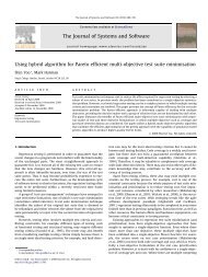
772 IEEE TRANSACTIONS ON SOFTWARE ENGINEERING, VOL. 36, NO. 6, NOVEMBER/DECEMBER 2010Fig. 4. Fault-detecting ability of statistical testing compared to uniform random testing (Experiment B). (a) simpleFunc, (b) bestMove, (c) nsichneu.a probability lower bound greater than or equal to the targetvalue, t cov given in Table 2). T þ is the mean time taken bythese successful runs (measured as CPU user time), and Tthe mean time taken by unsuccessful runs.We may consider each run of the algorithm to beequivalent to a flip of a coin where the probability of thecoin landing with “heads up” or of the algorithm finding asuitable distribution is þ . Trials such as these, where thereare two possible outcomes and they occur with fixedprobabilities, are termed Bernoulli trials [40]. In practice, afteran unsuccessful search, we would run another search with anew, different seed to the PRNG; in other words, we wouldperform a series of Bernoulli trials until one is successful. Thenumber of failures that occur before a successful outcome in aseries of Bernoulli trials follows a geometric distribution [40],with the mean number of failures being given by ð1 þ Þ= þ[41]. Therefore, we may calculate the mean time taken until asuccessful search occurs (including the time taken for thesuccessful search itself) as:C þ ¼ 1 þT þ T þ : ð11Þ þThe calculated values for C þ are given in the Table 3 and area prediction of how long, on average, it would take to find asuitable probability distribution.It is a conservative prediction in that it assumes theavailability of only one CPU core on which searches canbe run. Software engineers are likely to have access tosignificantly more computing resources than this, even ontheir desktop PC, which would allow searches to beperformed in parallel.We argue that the predicted time until success isindicative of practicality for all three SUTs. The longesttime—the value of C þ for nsichneu—is approximately10 hours, rising to 22 hours at extreme end of its confidenceinterval. These results provide strong evidence for Hypothesis1, that automated search can be a practical method ofderiving probability distributions for statistical testing.7.3 Experiment BThe results of Experiment B are summarized in Fig. 4.The upper row of graphs compares the mutation score oftest sets derived from statistical and uniform randomtesting over a range of test sizes. The mutation scores wereassessed at each integer test size in the range, but for clarity,error bars are shown at regular intervals only.The lower row of graphs show the p-value (left-hand axisusing a log scale) for the rank-sum test applied at each testsize, and the effect size A-statistic (right-hand axis). Dottedlines indicate a 5 percent p-value and the lower boundaries ofthe medium effect size regions. p-values below the 5 percentline indicate that the differences in the mutation scores arestatistically significant. A-statistic values above the 0.64 line,or below the 0.36 line, indicate a medium or large effect size.The graphs demonstrate statistically significant differencesin the mutation scores of test sets derived by statisticaland uniform random testing, with the former having the
POULDING AND CLARK: EFFICIENT SOFTWARE VERIFICATION: STATISTICAL TESTING USING AUTOMATED SEARCH 773greater fault-detecting ability for most test sizes. The effectsize is medium or large for many test sizes.These results support Hypothesis 2 that test setsgenerated using statistical testing are more efficient thantest sets generated by uniform random testing: For the sametest size, the former test sets typically have greater faultdetectingability.The exception is for larger test sets (size > 100) applied tonsichneu. For these larger test sets, uniform random testingis significantly more effective at detecting faults. We suspectthat this is due to a lack of diversity in the probabilitydistribution, and this motivates the use of a diversityconstraint during search.The horizontal dotted lines in the upper row of graphs inFig. 4 are the mean mutation score for each statistical test setat the size at which it first exercises all of the coverageelements in the SUT at least once. (The vertical dotted linesare the mean of these sizes.) At these sizes, the test setssatisfy the adequacy criterion of deterministic structuraltesting. However, due to the stochastic nature in which theyare generated, they will usually contain more test cases thana minimally sized test set. The additional test cases can onlyimprove the mutation score of the test set; therefore, theirmutation scores—the horizontal dotted line—represent anupper bound for the mutation scores achievable bydeterministic structural testing.For each SUT, the mutation scores obtained by statisticaltesting exceed this upper bound at sufficiently large testsizes. This is evidence in support of Hypothesis 3, that testsets derived using statistical testing where each coverageelement is exercised multiple times detect more faults thantest sets typical of deterministic structural testing thatexercise each element only once.7.4 Cost-Benefit AnalysisThe results of Experiments A and B taken together enable asimple cost-benefit analysis that compares statistical testingwith uniform random testing. This can be performed in anumber of ways: for example, by considering the differencein fault detecting ability of test sets of the same size for thetwo methods or the difference in the cost of testing for testsets of different size that have same fault detecting ability.We take the second of these two approaches in order toavoid speculation on the costs of later rectifying faults thatare not discovered during testing, as these costs are highlydependent on the context.If we choose a fault-detecting ability equivalent to amutation score of 0.55 for bestMove, the results of ExperimentB show that this occurs at a test size of 4 for statisticaltesting and at a test size of 61 for uniform random testing.(These sizes are obtained from the data used to plot thegraphs of Fig. 4b.) <strong>Statistical</strong> testing incurs a cost in findinga suitable probability distribution, and from Table 3, thissearch takes, on average, 129 minutes. If executing,and—often more significantly—checking the results of thetests against a specification or an oracle takes longer than129 minutes for the additional 57 test cases required byrandom testing, then statistical testing will be more efficientin terms of time. We argue that when checking test resultsinvolves a manual comparison against a specification, thenthe superior time efficiency of statistical testing is likely tobe realized in this case. We also note that the search for aprobability distribution is automated, requiring little or nomanual effort, and so speculate that statistical testing islikely to be superior in terms of monetary cost (even insituations where it is not superior in terms of time) if theexecution and checking of the additional 57 test cases is apredominantly manual, and therefore expensive, process.We may repeat this analysis for nsichneu, again choosing afault detecting ability equivalent to a mutation score of 0.55.In this case, random testing requires 14 more test cases thanstatistical testing: The test sizes are 66 and 52, respectively.The search for a probability distribution suitable for statisticaltesting takes 592 minutes. The superiority of statistical testingin terms of time is not as convincing for nsichneu: Randomtesting is quicker overall if executing and checking the extra14 test cases takes no longer than 10 hours. However, weagain note that the search for the probability distribution isautomated, and so, considering monetary cost, statisticaltesting may be cheaper than random testing if checking theresults of the extra 14 test cases is a manual process.The simple analyses of this section are dependent on themutation score we choose. Nevertheless, for bestMove, thelarge difference in the fault-detecting ability of the twomethods shown by Fig. 4b suggests that the generalconclusion remains the same for most choices of mutationscore. For nsichneu, however, any benefit of statistical testingis lost for mutation scores above approximately 0.6. As can beseen in Fig. 4c, mutation scores above this level are achievedby random testing with test sizes that are smaller than thoserequired by statistical testing. This underlines the importanceof investigating whether the use of a diversity constraintimproves the fault-detecting ability of statistical testing.7.5 Experiment CThe results of Experiment C are summarized in Fig. 5. Eachgraph shows the mutation scores for a sequence ofprobability distributions taken from the trajectory of onesearch run. The probability lower bound for each distribution(evaluated accurately using a large sample size) isplotted on the x-axis, and the mutation score (with errorbar) on the y-axis. The lines connect mean mutation scorescalculated at the same test size. Note that the left-hand pointin each graph is the uniform probability distribution that isused to initialize the search: This distribution is equivalentto that used for uniform random testing.At small values of the lower bound—at the left of thegraphs—mutation scores get better as the probability lowerbound increases. However, for larger values of the lowerbound at the right of Fig. 5c, the mutation score begins todecrease. There is also some evidence for this effect at thehighest lower bound values in Fig. 5b.We suspect that is because diversity can be lost as thesearch proceeds—the probability distribution is “overfitted”to the coverage constraint—and so, despite a highlower bound, the distribution generates test sets that arerelatively poor at detecting faults. This again motivates theuse of a diversity constraint in order to avoid this loss ofefficiency as the search proceeds.The results of Experiment C provide some evidence insupport of Hypothesis 4 that distributions with higher lowerbounds generate test sets with a greater ability to detectfaults. However, this is not true in all cases: <strong>Search</strong>ing fornear-optimal lower bounds can be counter-productive forsome SUTs, and we suspect this is a result of losing diversity.