Omitted Explanatory Variables, Multicollinearity, and Irrelevant ...

Chapter 14: Omitted Explanatory Variables, Multicollinearity, andIrrelevant Explanatory VariablesChapter 14 Outline• Reviewo Unbiased Estimation Procedures• Estimates and Random Variables• Mean of the Estimate’s Probability Distribution• Variance of the Estimate’s Probability Distributiono Correlated and Independent (Uncorrelated) Variables• Scatter Diagrams• Correlation Coefficient• Omitted Explanatory Variableso A Puzzleo Goal of Multiple Regression Analysiso Omitting Explanatory Variables and Bias• Multicollinearityo Perfectly Correlated Explanatory Variableso Highly Correlated Explanatory Variableso Earmarks of Multicollinearity• Irrelevant Explanatory Variables: Good News and Bad NewsChapter 14 Preview Questions1. Review the goal of multiple regression analysis. In words, explain what multiple regressionanalysis attempt to do?2. Recall that the presence of a random variable brings forth both bad news and good news.a. What is the bad news?b. What is the good news?3. Consider an estimate’s probability distribution. Review the importance of its mean andvariance:a. Why is the mean of the probability distribution important? Explain.b. Why is the variance of the probability distribution important? Explain.4. Suppose that two variables are positively correlated.a. In words, what does this mean?b. What type of graph do we use to illustrate their correlation? What does the graphlook like?c. What can we say about their correlation coefficient?d. When two variables are perfectly positively correlated, what will their correlationcoefficient equal?5. Suppose that two variables are independent (uncorrelated).a. In words, what does this mean?b. What type of graph do we use to illustrate their correlation? What does the graphlook like?c. What can we say about their correlation coefficient?

2Baseball Data: Panel data of baseball statistics for the 588 American League games played duringthe summer of 1996.Attendance tDateDay tDateMonth tDateYear tDayOfWeek tDH tHomeGamesBehind tHomeIncome tHomeLosses tHomeNetWins tHomeSalary tHomeWins tPriceTicket tVisitGamesBehind tVisitLosses tVisitNetWins tVisitSalary tVisitWins tPaid attendance for game tDay of game tMonth of game tYear of game tDay of the week for game t (Sunday=0, Monday=1, etc.)Designator hitter for game t (1 if DH permitted; 0 otherwise)Games behind of the home team for game tPer capita income in home team's city for game tSeason losses of the home team before the game for game tNet wins (wins less losses) of the home team before game tPlayer salaries of the home team for game t (millions of dollars)Season wins of the home team before the game for game tAverage price of tickets sold for game t‘s home team (dollars)Games behind of the visit team for game tSeason losses of the visit team before the game for game tNet wins (wins less losses) of the visiting team game tPlayer salaries of the visiting team for game t (millions of dollars)Season wins of the visiting team before the game6. Focus on the baseball data.a. Consider the following simple model:Attendance t= β Const+ β PricePriceTicket t+ e tAttendance depends only on the ticket price.1) What does the economist’s downward sloping demand curve theory suggestabout the sign of the PriceTicket coefficient, β Price?2) Use the ordinary least squares (OLS) estimation procedure to estimate themodel’s parameters. Interpret the regression results.Click here to access data {EViewsLink}

48. The following are excerpts from an article appearing in the New York Times on September 1,2008:Doubt Grow Over Flu Vaccine in Elderlyby Brenda GoodmanThe influenza vaccine, which has been strongly recommended for people over 65 formore than four decades, is losing its reputation as an effective way to ward off the virusin the elderly.A growing number of immunologists and epidemiologists say the vaccine probably doesnot work very well for people over 70 …The latest blow was a study in The Lancet last month that called into question much ofthe statistical evidence for the vaccine’s effectiveness.The study found that people who were healthy and conscientious about staying wellwere the most likely to get an annual flu shot. … [others] are less likely to get to theirdoctor’s office or a clinic to receive the vaccine.Dr. David K. Shay of the Centers for Disease Control and Prevention, a co-author of acommentary that accompanied Dr. Jackson’s study, agreed that these measures of health… “were not incorporated into early estimations of the vaccine’s effectiveness” and couldwell have skewed the findings.a. Intuitively, does being healthy and conscientious about staying well increase ordecrease the chances of getting flu? ___________Similarly, does being healthy and conscientious about staying well increase ordecrease the severity of the flu if an individual does get it? ___________b. According to the article, are those who are healthy and conscientious about stayingwell more or less likely to get a flu shot? ______________c. The article alleges that previous studies did not incorporate health and conscientiousin judging the effectiveness of flu shots. If the allegation is true, have previousstudies overestimated or underestimated the effectiveness of flu shots?________________

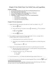
5Review: Unbiased Estimation ProceduresEstimates and Random VariablesEstimates are random variables. Consequently, there is both good news and bad news. Before thedata are collected and the parameters are estimated:• Bad news: We cannot determine the numerical values of the estimates with certainty(even if we knew the actual values of the constant and coefficients).• Good news: On the other hand, we can describe the probability distribution of theestimate telling us how likely it is for the estimate to equal its possible numerical values.Mean (Center) of the Estimate’s Probability DistributionAn unbiased estimation procedure does not systematicallyunderestimate or overestimate the actual value. The mean (center) ofthe estimate’s probability distribution equals the actual value; that is,when the experiment is repeated many, many times, the average ofthe numerical values of the estimates equals the actual value.When the distribution is symmetric, we can provide an interpretationthat is perhaps even more intuitive. If the experiment were repeatedmany, many times• half the time the estimate is greater than the actual value;• half the time the estimate is less than the actual value.Of course in reality, the experiment is only conducted once, only one regression is run.Accordingly, we can apply the relative frequency interpretation of probability:• When the estimation procedure is unbiased, the chances that the estimate will be greaterthan the actual value in a single regression equal the chances that the estimate will beless.The procedure does not systematically overestimate or underestimate the actual value.Variance (Spread) of the Estimate’s Probability Distribution VarianceActual ValueEstimateFigure 14.2: Probability Distribution foran Unbiased Estimation ProcedureWhen the estimationprocedure is unbiased,the distribution variance(spread) indicates theestimate’s reliability; thevariance tells us howlikely it is that thenumerical value of theestimate resulting fromone repetition of theexperiment will be closeto the actual value.Variance LargeEstimateActual ValueVariance large↓Small probability that theestimate from one repetitionof the experiment will beclose to the actual value↓Estimate is unreliableVariance SmallEstimateActual ValueVariance small↓Large probability that theestimate from one repetitionof the experiment will beclose to the actual value↓Estimate is reliableFigure 14.3: Probability Distribution of Estimates

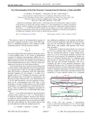
6Review: Correlated and Independent (Uncorrelated)VariablesTwo variables are• correlated whenever the value of one variable does help us predict the value of the other.• independent (uncorrelated) whenever the value of one variable does not help us predictthe value of the other;Examples of Correlated and Independent VariablesDow Jones and Nasdaq Growth RatesDeviations From Means20 NasdaqAmherst Precipitation and and Nasdaq Growth RateDeviations From Means20 Nasdaq10100Dow Jones-20 -10 0 10 200Precipitation-5 -4 -3 -2 -1 0 1 2 3 4 5-10-10-20-20Not Independent: Positively CorrelatedIndependent: UncorrelatedCorrCoef = .67 CorrCoef = –.07 ≈ 0Figure 14.1: Scatter Diagrams, Correlation, and IndependenceThe Dow Jones and Nasdaq growth rates are positively correlated. Most of the scatter diagrampoints lie in the first and third quadrants. When the Dow Jones growth rate is high, the Nasdaqgrowth rate is usually high also. Similarly, when the Dow Jones growth rate is low, the Nasdaqgrowth rate is usually low also. Knowing one growth rate helps us predict the other. On theother hand, Amherst precipitation and the Nasdaq growth rate are independent, uncorrelated.The scatter diagram points are spread rather evenly across the graph. Knowing the Nasdaqgrowth rate does not help us predict Amherst precipitation and vice versa.Correlation Coefficient: Indicates how correlated two variables are; the correlation coefficientranges from −1 to +1:• = 0: Independent (uncorrelated);Knowing the value of one variable does not help us predict the value of the other.• > 0: Positive correlation;Typically, when the value of one variable is high, the value of the othervariable will be high.• < 0: Negative correlation.Typically, when the value of one variable is high, the value of the othervariable will be low.

7Omitted Explanatory VariablesTo explain the omitted variable phenomena we shall consider baseball attendance data.Project: Assess the determinants of baseball attendance.Baseball Data: Panel data of baseball statistics for the 588 American League games playedduring the summer of 1996.Attendance tDateDay tDateMonth tDateYear tDayOfWeek tDH tHomeDivision tHomeGamesBehind tHomeIncome tHomeLosses tHomeNetWins tHomeSalary tHomeWins tPriceTicket tVisitDivision tVisitGamesBehind tVisitLosses tVisitNetWins tVisitSalary tVisitWins tPaid attendance for game tDay of game tMonth of game tYear of game tDay of the week for game t (Sunday=0, Monday=1, etc.)Designator hitter for game t (1 if DH permitted; 0 otherwise)Division of the home team for game tGames behind of the home team for game tPer capita income in home team's city for game tSeason losses of the home team before the game for game tNet wins (wins less losses) of the home team before game tPlayer salaries of the home team for game t (millions of dollars)Season wins of the home team before the game for game tAverage price of tickets sold for game t‘s home team (dollars)Division of the visit team for game tGames behind of the visit team for game tSeason losses of the visit team before the game for game tNet wins (wins less losses) of the visiting team game tPlayer salaries of the visiting team for game t (millions of dollars)Season wins of the visiting team before the gameA PuzzleLet us begin our analysis by focusing on the price of tickets. Consider the following two modelsthat attempt to explain game attendance:Model 1: Attendance depends on ticket price only.Attendance t= β Const+ β PricePriceTicket t+ e tDownward Sloping Demand Theory: This model is based on the economist’s downwardsloping demand theory. An increase in the price of a good decreases the quantity demand.Higher ticket prices should reduce attendance; hence, the PriceTicket coefficient should benegative:β Price< 0

8We shall use the ordinary least squares (OLS) estimation procedure to estimate the model’sparameters:Click here to access data {EViewsLink}Dependent variable: AttendanceExplanatory variable: PriceTicketDependent Variable: ATTENDANCEIncluded observations: 585Coefficient Std. Error t-Statistic Prob.PRICETICKET 1896.611 142.7238 13.28868 0.0000C 3688.911 1839.117 2.005805 0.0453Table 14.1: Baseball Regression Results – Ticket Price OnlyInterpretation: We estimate that $1.00 increase in the price of tickets increases by 1,897 pergame.The estimated coefficient for the ticket price is positive suggesting that higher prices lead toan increase in quantity demanded. This contradicts the downward sloping demand theory,does it not?Model 2: Attendance depends on ticket price and salary of home team.Attendance t= β Const+ β PricePriceTicket t+ β HomeSalaryHomeSalary t+ e tIn the second model, we include not only the price of tickets as an explanatory variable, butalso the salary of the home team. We can justify the salary explanatory variable in thegrounds that fans like to watch good players. We can call this the star effect. Presumably, ahigh salary team has better players, more stars, on its roster and accordingly will draw morefans.Star Theory: Teams with higher salaries will have better players which will increaseattendance. The HomeSalary coefficient should be positive:β HomeSalary> 0Now, use the ordinary least squares (OLS) estimation procedure to estimate the parameters.Dependent variable: AttendanceExplanatory variables: PriceTicket and HomeSalaryDependent Variable: ATTENDANCEIncluded observations: 585Coefficient Std. Error t-Statistic Prob.PRICETICKET -590.7836 184.7231 -3.198211 0.0015HOMESALARY 783.0394 45.23955 17.30874 0.0000C 9246.429 1529.658 6.044767 0.0000Table 14.2: Baseball Regression Results – Ticket Price and Home Team SalaryInterpretation: We estimate that a• $1.00 increase in the price of tickets decreases attendance by 591 per game.• $1 million increase in the home team salary increases attendance by 783 per game.

9These coefficients are consistent with our theories.The two models produce very different results concerning the effect of the ticket price onattendance. More specifically, the coefficient estimate for ticket price changes drastically from1,897 to −591 when we add home team salary as an explanatory variable. This is disquieting.Recall the goal of multiple regression analysis:Goal of Multiple Regression Analysis: Multiple regression analysis attempts to sort out theindividual effect of each explanatory variable. An explanatory variable’s coefficient estimateallows us to estimate the change in the dependent variable resulting from a change in thatparticular explanatory variable while all other explanatory variables remain constant.The estimate of an explanatory variable’s coefficient allows us to assess the effect that theexplanatory variable by itself has on the dependent variable.In Model 1 we estimate that a $1.00 increase in the ticket price increase attendance by nearly 2,000per game whereas in Model 2 we estimate that a $1.00 increase decreases attendance by 600 pergame. The two models suggest that the individual effect of the ticket price is very different.Obviously, this is a puzzle.Question: How can we rationalize this dramatic change?Answer: The omitted variable phenomenon provides the explanation.Claim: Omitting an explanatory variable from a regression will bias the estimation procedurewhenever two conditions are met. Bias results if the omitted explanatory variable:• influences the dependent variable;• is correlated with an included explanatory variable.When these two conditions are met, the coefficient estimate of the included explanatory variable isa composite of two effects; the coefficient estimate of the included explanatory variable reflects theinfluence that the• included explanatory variable actually has on the dependent variable (direct effect);• omitted explanatory variable has on the dependent variable because the includedexplanatory variable is acting as a proxy for the omitted explanatory variable (proxyeffect).Since the goal of multiple regression analysis is to sort out the individual effect of eachexplanatory variable we want to capture only the direct effect. We can now use the EconometricsLab to justify our claims concerning omitted explanatory variables.

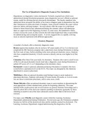
10Econometrics Lab 14.1: Omitted Variable Proxy EffectModel: y t= β Const+ β Coef1ExpVbl1 t+ β Coef2ExpVbl2 t+ e t{LabLink}By default the actual coefficient ofthe first explanatory variable,ExpVbl1, is positive, 2. We shall focuson this explanatory variable. Wewish to estimate the direct effect thatExpVbl1 has on the dependentvariable.Be certain that the “Both x’s”checkbox is cleared. The firstexplanatory variable, ExpVbl1, willnow be included in the regressionand the second, ExpVbl2 will beomitted. That is, ExpVbl1 is theincluded explanatory variable andExpVbl2 is the omitted explanatoryvariable. We shall consider threecases to illustrate when bias does anddoes not result:• Case 1. The coefficient of theomitted explanatory variableis nonzero and the twoexplanatory variables areindependent (uncorrelated).Act Coef 1PauseStart• Case 2. The coefficient of the omitted explanatory variable is zero and the twoexplanatory variables are correlated.• Case 3. The coefficient of the omitted explanatory variable is nonzero and the twoexplanatory variables are correlated.We claim that only in the last case does bias results because only in the last case is the proxyeffect is present.012Act Coef 2123RepetitionCoef1 Value EstMeanVarSample Size78910Ests Above Actual ValueEsts Below Actual ValueStopCorr12−.8−.4.0.4.8Is the estimationprocedure for thecoefficient valueunbiased?Variables1 and 2CorrelationParameterPercent ofEstimatesAboveand BelowActualValueBoth x’sFigure 14.4: Omitted Variable Simulation

11Case 1: Coefficient of the omitted explanatory variable is nonzero (β Coef2= 3).The two explanatory variables are independent (Corr12 = 0).Begin by focusing on the included explanatory variable, ExpVbl1. By default its actual coefficient,β Coef1, equals 2; the actual coefficient is positive. An increase in the included explanatory variable,ExpVbl1, increases the dependent variable, y. This is the effect we want to capture, the directeffect of the included explanatory variable on the dependent variable.What about a potential proxy effect? Since the two explanatory variables are independent(uncorrelated), the increase in the included explanatory variable, ExpVbl1, will not typically affectthe omitted explanatory variable, ExpVbl2. Therefore, there is no proxy effect and hence biasshould not result.ExpVbl1 tup → Typically, ExpVbl2 tunaffected↓ β Coef1> 0 Independent ↓ β Coef2> 0y tupy tunaffected↓Direct Effect↓No Proxy EffectIs our logic confirmed by the lab? By default, the actual coefficients for first explanatory variable,ExpVbl1, equals 2 and the actual coefficient for second explanatory variable, ExpVbl2, equals 3.The correlation parameter, Corr12, equals 0; hence, the two explanatory variables areindependent (uncorrelated). Be certain that the Pause checkbox is cleared. Click Start and aftermany, many repetitions, click Stop. Table 14.3 reports that the average value of the coefficientestimates for the first explanatory variable equals its actual value. Both equal 2.0. The ordinaryleast squares (OLS) estimation procedure is unbiased.MeanPercent of Coef1 EstimatesActual Actual Correlation (Average) of Coef 1 Below Actual Above ActualCoef 1 Coef 2 Coefficient Estimates Value Value2 3 .0 ≈2.0 ≈50.0 ≈50.0Table 14.3: Omitted Variables Simulation ResultsThe ordinary least squares estimation (OLS) procedure only captures the individual influencethat the first explanatory variable has on the dependent variable. This is precisely the effect thatwe wish to measure. In this case, the ordinary least squares estimation (OLS) procedure isunbiased; it is doing what we want it to do.Case 2: Coefficient of the omitted explanatory variable is zero (β Coef2= 0).The two explanatory variables are correlated (Corr12 = .4).In the second case, the two explanatory variables are positively correlated: when the firstexplanatory variable, ExpVbl1, increases, the second explanatory variable, ExpVbl2, will typicallyincrease also. But the actual coefficient of the omitted explanatory variable, β Coef2, equals 0; hence,the dependent variable, y, is unaffected by the increase in ExpVbl2. There is no proxy effectbecause the omitted variable does not affect the dependent variable; hence, bias should not result.ExpVbl1 tup → Typically, ExpVbl2 tup↓ β Coef1> 0 Positive correlation ↓ β Coef2= 0y tupy tunaffected↓Direct Effect↓No Proxy Effect

12In the simulation, correlation parameter is reset to .4, the two explanatory variables are positivelycorrelated; the actual coefficient of explanatory variable 2 is now set to 0. Click Start and aftermany, many repetitions, click Stop. Table 14.4 reports that the average value of the coefficientestimates for the first explanatory variable equals its actual value. Both equal 2.0. The ordinaryleast squares estimation procedure is unbiased.MeanPercent of Coef1 EstimatesActual Actual Correlation (Average) of Coef1 Below Actual Above ActualCoef 1 Coef 2 Coefficient Estimates Value Value2 3 .0 ≈2.0 ≈50.0 ≈50.02 0 .4 ≈2.0 ≈50.0 ≈50.0Table 14.4: Omitted Variables Simulation ResultsAgain, the ordinary least squares estimation (OLS) procedure captures the individual influencethat the first explanatory variable has on the dependent variable. Again, all is well.Case 3: Coefficient of the omitted explanatory variable is nonzero (β Coef2= 3).The two explanatory variables are correlated (Corr12 = .4).As with Case 2, the two explanatory variables are positively correlated; when the firstexplanatory variable, ExpVbl1, increases the second explanatory variable, ExpVbl2, will typicallyincrease also. But now, the actual coefficient of the omitted explanatory variable, β Coef2, is positive;hence, an increase ExpVbl2 in increases the dependent variable. There is a proxy effect.ExpVbl1 tup → Typically, ExpVbl2 tup↓ β Coef1> 0 Positive correlation ↓ β Coef2> 0y tupy tup↓Direct Effect↓Proxy EffectIn the simulation, the actual coefficient of explanatory variable 2 is once again 3. The twoexplanatory variables are still positively correlated. Click Start and after many, many repetitions,click Stop. Table 14.5 reports that the average value of the coefficient estimates for the firstexplanatory variable, 3.3, exceeds its actual value, 2.0. The ordinary least squares estimationprocedure is biased upward.MeanPercent of Coef1 EstimatesActual Actual Correlation (Average) of Coef1 Below Actual Above ActualCoef 1 Coef 2 Coefficient Estimates Value Value2 3 .0 ≈2.0 ≈50.0 ≈50.02 0 .4 ≈2.0 ≈50.0 ≈50.02 3 .4 ≈3.3 ≈12.5 ≈87.5Table 14.5: Omitted Variables Simulation ResultsNow we have a problem. The ordinary least squares (OLS) estimation procedure is overstatingthe influence of the first explanatory variable.

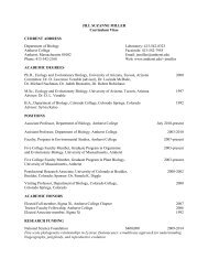
13Case 3 also allows us to illustrate what bias does and does not mean.• What bias does mean: Bias means that the estimation procedure systematicallyoverestimates or underestimates the actual value. In this case, upward bias is present. Theaverage of the estimates is greater than the actual value after many, many repetitions.• What bias does not mean: Bias doesnot mean that the value of the estimatein a single repetition must be less thanthe actual value in the case ofdownward bias or greater than theactual value in the case of upward bias.Focus on the last simulation. Theordinary least squares (OLS) estimationprocedure is biased upward as aconsequence of the proxy effect.Despite the upward bias, however, theestimate of the included explanatoryvariable is less than the actual value in12.5 percent of the repetitions. Upwardbias does not guarantee that in any onerepetition the estimate will be greaterthan the actual value. It just means thatb Coef1< 2it will be greater “on average.” If the probability distribution is symmetric, the chances ofthe estimate being greater than the actual value exceed the chances of being less.23.3Figure 14.5: Probability Distribution for an UpwardBiased Estimation Procedureb Coef1Now, let us summarize our three cases:Does the omitted Is the omitted Estimation procedurevariable influence the variable correlated with for the includedCase dependent variable? an included variable? Variable is1 Yes No Unbiased2 No Yes Unbiased3 Yes Yes BiasedTable 14.6: Omitted Variables Simulation SummaryEconometrics Lab 14.2: Avoiding Omitted Variable BiasQuestion: Is the estimation procedure biased or unbiased when both explanatory variables areincluded in the regression?{LabLink}To address this question, the Both x’s checkbox is now checked. This means that both explanatoryvariables, ExpVbl1 and ExpVbl2, will be included in the regression. Both explanatory variablesaffect the dependent variable and they are correlated. In this case, if one of the explanatoryvariables were omitted, bias would result. When both variables are included, however, theordinary least squares (OLS) estimation procedure is unbiased:Simulations: Both Explanatory Variables IncludedActual Actual Correlation Mean of Coef 1Coef 1 Coef 2 Parameter Estimates2 3 .4 ≈2.0Table 14.7: Omitted Variables Simulation Results – No Omitted VariablesConclusion: To avoid omitted variable bias, all relevant explanatory variables should be includedin a regression.

14Revisiting the baseball attendance regressionsReconsider our first baseball attendance model that included only ticket price.Model 1: Attendance t= β Const+ β PricePriceTicket t+ e tTheory: β Price< 0Baseball Data: Panel data of baseball statistics for the 588 American League games playedduring the summer of 1996.Attendance tPaid attendance at the game tPriceTicket tAverage price of tickets sold for game t‘s home team (dollars)HomeSalary tPlayer salaries of the home team for game t (millions of dollars)Click here to access data {EViewsLink}Dependent variable: AttendanceExplanatory variable: PriceTicketDependent Variable: ATTENDANCEIncluded observations: 585Coefficient Std. Error t-Statistic Prob.PRICETICKET 1896.611 142.7238 13.28868 0.0000C 3688.911 1839.117 2.005805 0.0453Table 14.8: EViews Baseball Regression Results – Ticket Price OnlyInterpretation: We estimate that $1.00 increase in the price of tickets increases by 1,897 pergame.Question: When ticket price is included in the regression and home team salary (star effect) isomitted, is there reason to believe that the estimation procedure for the ticket price coefficientmay be biased?We just learned that the bias results when an omitted explanatory variable:• influences the dependent variableand• is correlated with an included explanatory variable.It certainly appears reasonable to believe that home team salary, the star effect, will affectattendance. The club owner who is paying the high salaries certainly believes so. So now, let ususe statistical software to determine if ticket price and home team salary are correlated:Correlation MatrixPRICETICKET HOMESALARYPRICETICKET 1.000000 0.777728HOMESALARY 0.777728 1.000000Table 15.7: Ticket Price and Home Team Salary Correlation MatrixThe correlation coefficient between PriceTicket and HomeSalary is .78; the variables are positivelycorrelated. We can now apply the “omitted variable” logic:PriceTicket tup → Typically, HomeSalary tup↓ β Price< 0 Positive ↓ β HomeSalary> 0Attendance tdown correlation Attendance tup↓Direct Effect↓Proxy Effect

15As a consequence of the proxy effect, when HomeSalary is omitted from a regression, theprocedure to estimate the coefficient PriceTicket is biased upward; typically, the proxy effectpushes the price coefficient up, in the positive direction. The positive coefficient estimate couldresult as a consequence of the proxy effect.Now let us reexamine what occurs when both explanatory variables are included.Model 2: Attendance t= β Const+ β PricePriceTicket t+ β HomeSalaryHomeSalary t+ e tTheory: β Price< 0 and β HomeSalary> 0Dependent variable: AttendanceExplanatory variables: PriceTicket and HomeSalaryDependent Variable: ATTENDANCEIncluded observations: 585Coefficient Std. Error t-Statistic Prob.PRICETICKET -590.7836 184.7231 -3.198211 0.0015HOMESALARY 783.0394 45.23955 17.30874 0.0000C 9246.429 1529.658 6.044767 0.0000Table 14.2: Baseball Regression Results – Ticket Price and Home Team SalaryInterpretation: We estimate that a• $1.00 increase in the price of tickets decreases attendance by 591 per game.• $1 million increase in the home team salary increases attendance by 783 per game.The proxy effect is eliminated when the omitted explanatory variable is included.Omitted Variable Summary: Omitting an explanatory variable from a regression biases theestimation procedure whenever two conditions are met. Bias results if the omitted explanatoryvariable:• influences the dependent variable;• is correlated with an included explanatory variable.When these two conditions are met, the coefficient estimate of the included explanatory variable isa composite of two effects; the coefficient estimate of the included explanatory reflects the influencethat the• included explanatory variable actually has on the dependent variable (direct effect);• omitted explanatory variable has on the dependent variable because the includedexplanatory variable is acting as a proxy for the omitted explanatory variable (proxyeffect).The bad news is that the proxy effect leads to bias. The good news is that we can eliminate theproxy effect and its accompanying bias by including the omitted explanatory variable. But now,we shall learn that if two explanatory variables are highly correlated a different problem canemerge.

16MulticollinearityThe phenomenon of multicollinearity occurs when two explanatory variables are highlycorrelated. Recall that multiple regression analysis attempts to sort out the influence of eachindividual explanatory variable. But what happens when we include two explanatory variablesin a single regression that are perfectly correlated? Let us see.Perfectly Correlated Explanatory VariablesIn our baseball attendance workfile, ticket prices, PriceTicket, are reported in terms of dollars.Generate a new variable, PriceCents, that report ticket prices in terms of cents rather than dollars:PriceCents = 100 × PriceTicketNote that the variables PriceTicket and PriceCents are perfectly correlated. If we know one we canperfectly predict the value of the other. Just to be certain that this is true, use statistical softwareto calculate the correlation matrix:Correlation MatrixPriceTicket PriceCentsPriceTicket 1.000000 1.000000PriceCents 1.000000 1.000000Table 14.10: EViews Dollar and Cent Ticket Price Correlation MatrixThe correlation coefficient of PriceTicket and PriceCents equals 1.00. The variables are indeedperfectly correlated.Now, run a regression with Attendance as the dependent variable and both PriceTicket andPriceCents as explanatory variables.Dependent variable: AttendanceExplanatory variables: PriceTicket and PriceCentsYour statistical software will report a diagnostic. Different software packages provide differentmessages, but basically the software is telling us that it cannot run the regression.

17Why does this occur? The reason is that the two variables are perfectly correlated. Knowing thevalue of one allows us to predict perfectly the value of the other. Both explanatory variablescontain precisely the same information. Multiple regression analysis attempts to sort out theinfluence of each individual explanatory variable. But if both variables contain precisely the sameinformation, it is impossible to do this. How can we possibility separate out each variable’sindividual effect when the two variables contain identical information? We are asking statisticalsoftware to do the impossible.Explanatory variablesperfectly correlated↓Knowing the value of oneexplanatory value allowsus to predict perfectly thevalue of the other↓Both variables containprecisely the same information↓Impossible to separate outthe individual effect of eachNext, we consider a case in which the explanatory variables are highly, although not perfectly, correlated.Highly Correlated Explanatory VariablesWe focus attention on two variables included in our baseball data and theorize about how theyaffect attendance:Baseball Data: Panel data of baseball statistics for the 588 American League games playedduring the summer of 1996.Attendance tHomeNetWinsHomeGamesBehindPaid attendance for game tThe difference between the number of wins and losses of thehome team.The number of games the home team trails the first place team inthe home team’s divisionThe variable HomeNetWins captures the quality of the team. This variable will be positive andlarge for a high quality team. On the other hand, HomeNetWins will be a negative number for alow quality team. Since baseball fans enjoy watching high quality teams, we would expect highquality teams to be rewarded with greater attendance:Team Quality Theory: An increase in HomeNetWins increases Attendance.

18The variable HomeGamesBehind captures the home team’s standing in its divisional race. For thosewho are not baseball fans, note that all teams that win their division automatically qualify for thebaseball playoffs. Ultimately, the two teams what win the American and National Leagueplayoffs meet in the World Series. Since it is the goal of every team to win the World Series, eachteam strives to win its division. Games behind indicates how close a team is to winning itsdivision. To explain how games behind are calculated, consider the final standings of theAmerican League Eastern Division in 2009:Team Wins Losses Home Net Wins Games BehindNew York Yankees 103 59 44 0Boston Red Sox 95 67 28 8Tampa Bay Rays 84 78 6 19Toronto Blue Jays 75 87 −12 28Baltimore Orioles 64 98 −34 39Table 14.11: 2009 Final Season Standings – AL EastThe Yankees had the best record; the games behind value for the Yankees equals 0. The Red Soxwon eight fewer games than the Yankees; hence, the Red Sox were 8 games behind. The Rayswon 19 fewer games than the Yankees; hence the Rays were 19 games behind. Similarly, the BlueJays were 28 games behind and the Orioles 39 games behind. 5 During the season if a team’sgames behind becomes larger, it becomes less likely the team will win its division, less likely forthat team to qualify for the playoffs, and less likely for that team to eventually win the WorldSeries. Consequently, if a team’s games behind becomes larger, we would expect home team fansto become discourage resulting in less attendance:Division Race Theory: Increase in HomeGamesBehind decreases Attendance.We would expect HomeNetWins and HomeGamesBehind to be negatively correlated. AsHomeNetWins fall, a team moves farther from the top of its division and consequentlyHomeGamesBehind increase. We would expect the correlation coefficient for HomeNetWins andHomeGamesBehind to be negative. Let us check:Click here to access data {EViewsLink}HOMENETWINS HOMEGAMESBEHINDHOMENETWINS 1.000000 -0.962037HOMEGAMESBEHIND -0.962037 1.000000Table 14.12: HomeNetWins and HomeGamesBehind Correlation MatrixTable 14.12 reports that HomeGamesBehind and HomeNetWins are indeed negatively correlated aswe suspected. Furthermore, recall that the correlation coefficient must lie between −1 and +1.When two variables are perfectly negatively correlated their correlation coefficient equals −1.While HomeGamesBehind and HomeNetWins are not perfectly negatively correlated, they comeclose; they are very highly negatively correlated.We shall now use multiple regression analysis to sort out the individual influences that homewins less losses and games behind have on attendance. Our model now has four explanatoryvariables: PriceTicket, HomeSalary, HomeNetWins, and HomeGamesBehind.5In this example all teams have played the same number of games. When a different number ofgames have been played the calculation becomes a little more complicated. Games behind for anon-first place team equals(Wins of First − Wins of Trailing) + (Losses of Trailing − Losses of First)2

19Attendance t= β Const+ β PricePriceTicket t+ β HomeSalaryHomeSalary t+ β HomeNWHomeNetWins t+β HomeGBHomeGamesBehind t+ e tOur theories suggest that the coefficient for HomeSalary tshould be positive and the coefficient forHomeGamesBehind tshould be negative:Team Quality Theory: More net wins increase attendance. β HomeNW> 0.Division Race Theory: More games behind decreases attendance. β HomeGB< 0.We use the ordinary least squares estimation procedure (OLS) to estimate the model’s parameters:Dependent variable: AttendanceExplanatory variables: PriceTicket and HomeSalaryDependent Variable: ATTENDANCEIncluded observations: 585Coefficient Std. Error t-Statistic Prob.PRICETICKET -437.1603 190.4236 -2.295725 0.0220HOMESALARY 667.5796 57.89922 11.53003 0.0000HOMENETWINS 60.53364 85.21918 0.710329 0.4778HOMEGAMESBEHIND -84.38767 167.1067 -0.504993 0.6138C 11868.58 2220.425 5.345184 0.0000Table 14.13: Attendance Regression ResultsInterpretation: We estimate that a• $1.00 increase in the price of tickets decreases attendance by 437 per game.• $1 million increase in the home team salary increases attendance by 668 per game.• 1 additional net win increases attendance by 61.• 1 fewer game behind increases attendance by 84.The sign of each estimate supports the theories. Focus on the two new variables included in the model:HomeNetWins and HomeGamesBehind. Construct the null and alternative hypotheses.H 0: β HomeNW= 0 HomeNetWins has no effect on AttendanceH 1: β HomeNW> 0 HomeNetWins increases AttendanceH 0:β HomeGB= 0H 1: β HomeGB< 0HomeGamesBehind has no effect on AttendanceHomeGamesBehind decreases AttendanceWhile the signs are encouraging, some of results are disappointing:• The coefficient estimate for HomeNetWins is positive supporting our theory, but whatabout the Prob[Results IF H 0True]?What is the probability that the estimate from one regression would equal 60.53 ormore, if the H 0were true (that is, if the actual coefficient, β HomeNW, equals 0, if hometeam quality has no effect on attendance)? Using the tails probability:Prob[Results IF H 0True] = .47782≈ .24We cannot reject the null hypothesis at the traditional significance levels of 1, 5, or 10percent, suggesting that it is quite possible for the null hypothesis to be true, quitepossible that home team quality has no effect on attendance.

20• Similarly, The coefficient estimate for HomeGamesBehind is negative supporting ourtheory, but what about the Prob[Results IF H 0True]?What is the probability that the estimate from one regression would equal −84.39 orless, if the H 0were true (that is, if the actual coefficient, β HomeGB, equals 0, if gamesbehind has no effect on attendance)? Using the tails probability:Prob[Results IF H 0True] = .61382≈ .31Again, we cannot reject the null hypothesis at the traditional significance levels of 1,5, or 10 percent, suggesting that it is quite possible for the null hypothesis to be true,quite possible that games behind has no effect on attendance.Should we abandon our “theory” as a consequence of these regression results?Let us perform a Wald test the proposition that both coefficients equal 0:H 0: β HomeNW= 0 and β HomeGB= 0H 1: β HomeNW≠ 0 and/or β HomeGB≠ 0Neither team quality nor games behind have an effecton attendanceEither team quality and/or games behind have aneffect on attendanceWald Test:Test Statistic Value DF ProbabilityF-statistic 111.4021 (2, 580) 0.0000Table 14.14: EViews Wald Test ResultsProb[Results IF H 0True]: What is the probability that the F-statistic would be 111.4 or more, if theH 0were true (that is, if both β HomeNWand β HomeGBequal 0, if both team quality and games behindhave no effect on attendance)?Prob[Results IF H 0True] < .0001It is unlikely that the null hypothesis is true; it is unlikely that both team quality and gamesbehind have no effect on attendance.Paradox: Our t-tests and the Wald test are providing us with a paradoxical result:t-testsWald testCannot reject the Cannot reject the Can reject the nullnull hypothesis null hypothesis hypothesis that boththat team quality that games behind team quality and gameshave no effect have no effect behind have no effecton attendance. on attendance. on attendance.↓Team quality and/orIndividually, neither team quality nor games games behind do appear tobehind appear to influence attendanceinfluence attendanceIndividually, neither team quality nor games behind appears to influence attendancesignificantly; but taken together by asking if team quality and/or games behind influenceattendance, we conclude that they do.

21Next, let us run two regressions each of which includes only one of the two troublesomeexplanatory variables:Dependent Variable: ATTENDANCEIncluded observations: 585Coefficient Std. Error t-Statistic Prob.PRICETICKET -449.2097 188.8016 -2.379268 0.0177HOMESALARY 672.2967 57.10413 11.77317 0.0000HOMENETWINS 100.4166 31.99348 3.138658 0.0018C 11107.66 1629.863 6.815087 0.0000Table 14.15: EViews Attendance Regression Results – Home Wins Less Losses OnlyDependent Variable: ATTENDANCEIncluded observations: 585Coefficient Std. Error t-Statistic Prob.PRICETICKET -433.4971 190.2726 -2.278295 0.0231HOMESALARY 670.8518 57.69106 11.62835 0.0000HOMEGAMESBEHIND -194.3941 62.74967 -3.097931 0.0020C 12702.16 1884.178 6.741486 0.0000Table 14.16: EViews Attendance Regression Results – Home Games Behind OnlyWhen only a single explanatory variable is included the coefficient is significant.“Earmarks” of Multicollinearity – Explanatory Variables Highly CorrelatedWe are observing the earmarks of what is called multicollinearity:• Explanatory variables are highly correlated.• Regression with both explanatory variableso t-tests do not allow us to reject the null hypothesis that the coefficient of eachindividual variable equals 0; when considering each explanatory variableindividually, we cannot reject the hypothesis that each individually has noinfluence.o a Wald test allows us to reject the null hypothesis that the coefficients of bothexplanatory variables equal 0; when considering both explanatory variablestogether, we can reject the hypothesis that they have no influence.• Regressions with only one explanatory variable appear to produce “good” results.How can we explain this? Recall that multiple regression analysis attempts to sort out theinfluence of each individual explanatory variable. When two explanatory variables are perfectlycorrelated, it is impossible for the ordinary least squares (OLS) estimation procedure to separateout the individual influences of each variable. Consequently, if two variables are highly correlate,as team quality and games behind are, it may be very difficult for the ordinary least squares(OLS) estimation procedure to separate out the individual influence of each explanatory variable.This difficulty evidences itself in the probability distributions of the coefficient estimates. Whentwo highly correlated variables are included in the same regression, the variances of eachestimate’s probability distribution is large. This explains the large tails probabilities.

22Explanatory variablesperfectly correlated↓Knowing the value of onevariable allows us topredict the other perfectly↓Both variables containthe same information↓Impossible to separate outtheir individual effectsExplanatory variableshighly correlated↓Knowing the value of onevariable allows us topredict the other very accurately↓In some sense, both variablescontain nearly the same information↓Difficult to separate outtheir individual effects↓Large variance of each coefficientestimate’s probability distributionWe can use a simulation to justify our explanation.Econometrics Lab 14.3: MulticollinearityModel: y = β Const+ β Coef1ExpVbl1 t+ β Coef2ExpVbl2 t+ e t{LabLink}Focus on the two coefficients of the two x’s; by default:β Coef1= 2 β Coef2= 3Note that the Both x’s checkbox is checked indicatingthat both explanatory variables are included in theregression. Initially, the correlation coefficient isspecified as 0; that is, initially the explanatory variablesare independent. Be certain that the Pause checkbox iscleared and click Start. After many, many repetitionsclick Stop. Next, repeat this process for a correlationcoefficient of .4 and a correlation coefficient of .8.Mean of Variance ofCorrelation Coef 1 Coef 1Actual Coef 1 Parameter Estimates Estimates2 0 ≈2.0 ≈1.32 .4 ≈2.0 ≈2.72 .8 ≈2.0 ≈14.3Table 14.17: Multicollinearity Simulation ResultsAct Coef 1012Act Coef 2123RepetitionCoef 1 Value EstMeanVarSample SizePauseStart78910Both x’sStopCorr12−.8−.40.4.8Variables1 and 2CorrelationParameterFigure 14.6: Multicollinearity SimulationBy exploiting the relative frequency interpretation of probability, the simulation reveals bothgood news and bad news:• Good news: The ordinary least squares (OLS) estimation procedure is unbiased. Themean of the estimate’s probability distribution equals the actual value. The estimationprocedure does not systematically underestimate or overestimate the actual value.• Bad news: As the two explanatory variables become more correlated, the variance of thecoefficient estimate’s probability distribution increases. Consequently, the estimate fromone repetition becomes less reliable.The simulation illustrates the phenomenon of multicollinearity.

23Irrelevant Explanatory VariablesAn irrelevant explanatory variable is a variable that does not influence the dependent variable.Intuitively, including an irrelevant explanatory variable can be viewed as adding “noise,” anadditional element of uncertainty, into the mix. We can think of an irrelevant explanatoryvariable as adding a new random influence to the model. If our intuition is correct, it should leadto both good news and bad news:• Good news: Random influences do not cause the ordinary least squares (OLS) estimationprocedure to be biased. Consequently, the inclusion of an irrelevant explanatory variabledoes not lead to bias.• Bad news: The additional uncertainty added by the new random influence means thatthe coefficient estimate is less reliable; the variance of the coefficient estimate’sprobability distribution rises when an irrelevant explanatory variable is present.We shall use our Econometrics Lab to justify our intuition.Econometrics Lab 14.4: Irrelevant Explanatory VariablesConsider a two explanatory variable model:Model: y = β Const+ β Coef1ExpVbl1 t+ β Coef2ExpVbl2 t+ e tLet ExpVbl1 be the relevant explanatory variable andExpVbl2 be the irrelevant explanatory variable. The actualcoefficient of an irrelevant explanatory variable equals 0since the irrelevant explanatory variable has no effect onthe dependent variable:β Coef2= 0.By default the actual coefficient of the relevantexplanatory variable, ExpVbl1, equals 2:β Coef1= 2.Act Coef 1Sample SizePauseRepetitionCoef 1 Value Est−.8 VariablesAccess the lab:Mean−.4 1 and 2Var0 Correlation{LabLink}.4 ParameterInitially, the “Both x’s” checkbox is cleared indicating thatBoth x’s .8only the relevant explanatory variable, ExpVbl1, isincluded in the regression. Then, we investigate whathappens when the irrelevant explanatory variable isFigure 14.7: Irrelevant Explanatory Variable Labincluded by checking the “Both x’s” checkbox. In eachcase, we consider three correlation parameters: 0, .4, and .8. Table 14.18 reports the lab results.Only Coef1 Included Both Coef1 and Coef2 IncludedCorrelation Mean of Variance of Mean of Variance ofParameter for Coef 1 Coef 1 Coef 1 Coef 1Actual Coef 1 Variables 1 and 2 Estimates Estimates Estimates Estimates2.0 0 ≈2.0 ≈1.1 ≈2.0 ≈1.32.0 .4 ≈2.0 ≈1.1 ≈2.0 ≈2.72.0 .8 ≈2.0 ≈1.1 ≈2.0 ≈14.3Table 14.18: Irrelevant Explanatory Variable Simulation Results012Act Coef 2012Start78910StopCorr12

24The results reported in Table 14.18 are not surprising; the results support our intuition:• Only Relevant Variable (Variable 1) Included:o The mean of the coefficient estimates for relevant explanatory variable, ExpVbl1,equals 2, the actual value; consequently, the ordinary least squares (OLS)estimation procedure for the coefficient estimate is unbiased.o The variance of the coefficient estimates is not affect by the correlation betweenthe relevant and irrelevant explanatory variables because the irrelevantexplanatory variable is not included in the regression.• Both Relevant and Irrelevant Variables (Variables 1 and 2) Included:o The mean of the coefficient estimates for relevant explanatory variable, ExpVbl1,still equals 2, the actual value; consequently, the ordinary least squares (OLS)estimation procedure for the coefficient estimate is unbiased.o The variance of the coefficient estimates is greater whenever the irrelevantexplanatory variable is included.o Furthermore, we can now apply what we learned about multicollineaity. As thecorrelation between the relevant and irrelevant explanatory variables increases itbecomes more difficult for the ordinary least squares (OLS) estimation procedureto separate out the individual effects of each explanatory variable; consequently,the variance of each coefficient estimate’s probability distribution increases.The simulation illustrates the effect of including an irrelevant explanatory variable in a model.While it does not cause bias, it does make the coefficient estimates of the relevant explanatoryvariable less reliable by increasing the variance of its probability distribution.

25Chapter 14 Review Questions1. Consider an omitted explanatory variable:a. What problem can arise?b. Under what circumstances will the problem arise?2. Suppose that multicollinearity is present in a regression.a. What is the “good news?”b. What is the “bad news?”3. Suppose that an irrelevant explanatory variable is included in a regression.a. What is the “good news?”b. What is the “bad news?”Chapter 14 ExercisesCigarette Consumption Data: Cross section of per capita cigarette consumption and prices infiscal year 2008 for the 50 states and the District of Columbia.CigConsPC tEducCollege tEducHighSchool tIncPC tPop tPriceConsumer tPriceSupplier tRegionMidWest tRegionNorthEast tRegionSouth tRegionWest tSmokeRateAdult tSmokeRateYouth tState tTax tTobProdPC tCigarette consumption per capita in state t (packs)Percent of population with bachelor degrees in state tPercent of population with high school diplomas in state tIncome per capita in state t (1,000’s of dollars)Population of state t (persons)Price of cigarettes in state t paid by consumers (dollars per pack)Price of cigarettes in state t received by suppliers (dollars per pack)1 if state t in Midwest census region, 0 otherwise1 if state t in Northeast census region, 0 otherwise1 if state t in South census region, 0 otherwise1 if state t in West census region, 0 otherwisePercent of adults who smoke in state tPercent of youths who smoke in state tName of state tCigarette tax rate in state t (dollars per pack)Per capita tobacco production in state t (pounds)

261. Consider the following model:CigConsPC t= β Const+ β PricePriceConsumer t+ β EduCollEducCollege t+ β TobProdTobProdPC t+ e ta. Develop a theory that explains how each explanatory variable affects per capitacigarette consumption. What do your theories suggest about the sign of eachcoefficient?b. Use the ordinary least squares (OLS) estimation procedure to estimate theparameters of the model.Click here to access data {EViewsLink}c. Formulate the null and alternative hypotheses.d. Calculate Prob[Results IF H 0True] and assess your theories.2. Consider a second model explaining cigarette consumption:CigConsPC t= β Const+ β PricePriceConsumer t+ β IIncPC t+ β TobProdTobProdPC t+ e ta. Develop a theory that explains how each explanatory variable affects per capitacigarette consumption. What do your theories suggest about the sign of eachcoefficient?b. Use the ordinary least squares (OLS) estimation procedure to estimate theparameters of the model.Click here to access data {EViewsLink}c. Formulate the null and alternative hypotheses.d. Calculate Prob[Results IF H 0True] and assess your theories.3. Consider a third model explaining cigarette consumption:CigConsPC t= β Const+ β PricePriceConsumer t+ β EduCollEducCollege t+ β IIncPC t+β TobProdTobProdPC t+ e ta. Develop a theory that explains how each explanatory variable affects per capitacigarette consumption. What do your theories suggest about the sign of eachcoefficient?b. Use the ordinary least squares (OLS) estimation procedure to estimate theparameters of the model.Click here to access data {EViewsLink}c. Formulate the null and alternative hypotheses.d. Calculate Prob[Results IF H 0True] and assess your theories.

274. Focus on the coefficient estimates of EducCollege and IncomePC in exercises 1, 2, and 3.a. Compare the estimates.b. Provide a scenario to explain why the estimates may have changed as they did.House Earmark Data: Cross section data of proposed earmarks in the 2009 fiscal year for the 451House members of the 110 th Congress.CongressName tName of Congressperson tCongressParty tParty of Congressperson tCongressState tState of Congressperson tDollarsSolo tDollar value of earmarks received that were sponsored solely byCongressperson tDollarsSoloOthers tDollar value of earmarks received that were sponsored solely byCongressperson t plus earmarks with other CongresspersonsDollarsSoloOthersPres tDollar value of earmarks received that were sponsored solely byCongressperson t plus earmarks with other Congresspersons plusearmarks with the PresidentIncPC tIncome per capita in Congressperson t’s state (Dollars)NonState t1 if Congressperson t does not represent a state; 0 otherwiseNumberSolo tNumber of earmarks received that were sponsored solely byCongressperson tNumberSoloOthers tNumber of earmarks received that were sponsored solely byCongressperson t plus earmarks with other CongresspersonsNumberSoloOthersPres tNumber of earmarks received that were sponsored solely byCongressperson t plus earmarks with other Congresspersons plusearmarks with the PresidentPartyDem t1 if Congressperson t Democrat, 0 otherwisePartyInd t1 if Congressperson t Independent, 0 otherwisePartyRep t1 if Congressperson t Republican, 0 otherwiseRegionMidwest t1 if Congressperson t represents a midwestern state, 0 otherwiseRegionNortheast t1 if Congressperson t represents a northeastern state, 0 otherwiseRegionSouth t1 if Congressperson t represents a southern state, 0 otherwiseRegionWest t1 if Congressperson t represents a western state, 0 otherwiseScoreLiberal tCongressperson’s t liberal score rating in 2007Terms tNumber of terms served by Congressperson t in the U. S. CongressUnemRate tUnemployment rate in Congressperson t’s stateVoteDem tDemocratic vote percent in Congressperson t’s state in 2004Presidential electionVoteRep tRepublican vote percent in Congressperson t’s state in 2004Presidential election

285. Consider the following model explaining the number of solo earmarks:NumberSolo t= β Const+ β TermsTerms t+ β LiberalScoreLiberal t+ e ta. Develop a theory that explains how each explanatory variable affects the number ofsolo earmarks. What do your theories suggest about the sign of each coefficient?b. Use the ordinary least squares (OLS) estimation procedure to estimate theparameters of the model.Click here to access data {EViewsLink}c. Formulate the null and alternative hypotheses.d. Calculate Prob[Results IF H 0True] and assess your theories.6. Consider a second model explaining the number of solo earmarks:NumberSolo t= β Const+ β TermsTerms t+ β DemPartyDemocrat t+ e ta. Develop a theory that explains how each explanatory variable affects the number ofsolo earmarks. What do your theories suggest about the sign of each coefficient?b. Use the ordinary least squares (OLS) estimation procedure to estimate theparameters of the model.Click here to access data {EViewsLink}c. Formulate the null and alternative hypotheses.d. Calculate Prob[Results IF H 0True] and assess your theories.7. Consider a third model explaining the number of solo earmarks:NumberSolo t= β Const+ β TermsTerms t+ β LiberalScoreLiberal t+ β DemPartyDemocrat t+ e ta. Develop a theory that explains how each explanatory variable affects the number ofsolo earmarks. What do your theories suggest about the sign of each coefficient?b. Use the ordinary least squares (OLS) estimation procedure to estimate theparameters of the model.Click here to access data {EViewsLink}c. Formulate the null and alternative hypotheses.d. Calculate Prob[Results IF H 0True] and assess your theories.8. Focus on the coefficient estimates of ScoreLiberal and PartyDemocrat in exercises 5, 6, and 7.a. Compare the standard errors.b. Provide a scenario to explain why the standard errors may have changed as they did.