Counterexamples to a Likelihood Theory of Evidence

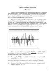
For each hypothesis, the likelihood is obtained by multiplying the probabilities ofthe data points together, where each probability has the form:PF( x< X < x+ dx, y< Y < y+ dy) = k pF( x, y),PB( x< X < x+ dx, y< Y < y+ dy) = k pB( x, y),where k = dxdy. Furthermore,pF( xy , ) = pF( xp )F( y| x), and pB( xy , ) = pB( yp )B( x| y).Since B2has a lower likelihood than F 2, it must be because pB( y ) is smaller than pF( x ) ,on average.This is odd because thespecification of marginalx − ydistributions, pB( y ) and pF( x ) is notwhat we think of as the essential2content of a ‘causal’ hypothesis. Thefalsity of B2is already apparent fromthe pattern that forms when the xyvalues are generated from y values,even we look at a narrow range of yvalues. The x values do not varyrandomly to the left and to the right ofthe line Y = X, as B2claims. Instead,they vary randomly to the left and theright of the line Y = 2X with half thevariance, just as we would expect if B1were true. This is easily seen byplotting residuals (x − y) against y (see Fig. 4). The residual variance is equal to 1because it is sum of two terms— one due to the deviation of the line Y = 2X from the lineY = X (the ‘explainable’ variation) and the other due to the smaller random variationabout the line Y = 2X. In contrast, if we were to plot the y residuals against x, then therewould be no discernible correlation between the y residuals and x.Example 3: We will have a counterexample to LTE if the competing hypothesescan be constructed so that the marginal components of their likelihoods are the same.Suppose that we are told an alternative story about how the marginal values aregenerated. According to this version of the Forward hypothesis, the x values are readfrom a predetermined list of values, and then a slight stochastic element imposed on thefinalvalue by randomly generating a small error from a uniform distribution of (small) width δaround the listed value. That is, X has a uniform distribution between the listed valueminus δ 2 and the listed value plus δ 2 . If we define ε = 1 δ , then for all observed x,P ( ) Fx = εdx. Similarly, B asserts that y values are first drawn from a list and thenrandomized in the same way, so that PB( y)= εdy. The story about how the othervariable is generated is the same as in Example 2, in each case. Now, we are told thatone of these hypotheses is true. Can we tell which one? Yes, by looking at the behaviorof the residuals (as explained in Example 2). Can we tell if we are just given the-2Figure 4: The x residuals (x − y) plotted as afunction of y. The residual has an averagevariation of 1, but the variation varies in asystematic way for different values of y.14