Counterexamples to a Likelihood Theory of Evidence

Counterexamples to a Likelihood Theory of EvidenceFinal Corrections, August 30, 2006. Forthcoming in Minds and Machines.MALCOLM R. FORSTER 1Department of Philosophy, University of Wisconsin-Madison, 5185 Helen C. White Hall,600 North Park Street, Madison WI 53706 USA. Email: mforster@wisc.eduAbstract: The Likelihood Theory of Evidence (LTE) says, roughly, that all theinformation relevant to the bearing of data on hypotheses (or models) is contained in thelikelihoods. There exist counterexamples in which one can tell which of two hypothesesis true from the full data, but not from the likelihoods alone. These examples suggest thatsome forms of scientific reasoning, such as the consilience of inductions (Whewell,1858), cannot be represented within Bayesian and Likelihoodist philosophies of science.Key words: The likelihood principle, the law of likelihood, evidence, Bayesianism,Likelihoodism, curve fitting, regression, asymmetry of cause and effect.IntroductionConsider two simple hypotheses, h 1 and h 2 , with likelihoods denoted by PE ( | h1)andPE ( | h2)respectively, where E is the total observed data—the actual evidence. Bydefinition, a simple statistical or probabilistic hypothesis has a precisely specifiedlikelihood (as opposed to composite hypotheses, or models, which do not—see below).If a hypothesis contains a free, or adjustable, parameter, such that different values wouldchange its likelihood, then it is not a simple hypothesis. The term “simple” is standardlyused in the classical statistics literature in this way—it does not mean that the hypothesisis simple in any intuitive sense, and it does not imply that the evidence is simple or thatthe relationship with the hypothesis is simple, or that its evidence is simple.A likelihood theory of evidence (LTE) is presupposed by the standard Bayesianmethod of comparing hypotheses, according to which two simple hypotheses arecompared by their posterior probabilities, Ph (1| E ) and Ph (2| E ). Bayes theorem tells usthat1 Thanks go to all those who responded well to the first version of this paper presented at the University ofPittsburgh Center for Philosophy of Science on January 31, 2006, and especially to Clark Glymour. Arevised version was presented at Carnegie-Mellon University on April 6, 2006. I also wish to thank JasonGrossman, John Norton, Teddy Seidenfeld, Elliott Sober, Peter Vranas, and three anonymous referees forvaluable feedback on different parts of the manuscript.This paper is part of the ongoing development of a half-baked idea about cross-situational invariance incausal modeling introduced in Forster (1984). I appreciated the encouragement at that time from Jeff Bub,Bill Demopoulos, Michael Friedman, Bill Harper, Cliff Hooker, John Nicholas, and Jim Woodward. CliffHooker discussed the idea in his (1987), and Jim Woodward suggested a connection with statistics, whichhas taken me 20 years to figure out.

Ph (1| E) Ph (1) PE ( | h1)= × .Ph (2| E) Ph (2) PE ( | h2)Thus, the evidence, E, affects the comparison of hypotheses only via their likelihoods.Once the likelihoods are given, the detailed information contained in the data is no longerrelevant. That is roughly the thesis stated by Barnard (1947, p. 659):The connection between a simple statistical hypothesis H and observedresults R is entirely given by the likelihood, or probability functionL(R|H). If we make a comparison between two hypotheses, H and H′, onthe basis of observed results R, this can be done only by comparing thechances of, getting R, if H were true, with those of getting R, if H′weretrue.If the likelihood of a hypothesis is viewed as a measure of fit with the data, then LTEsays that the impact of evidence on hypothesis comparison depends only on how well thehypotheses fit the total observed data. It is a surprising thesis, because it implies that theevidence relation between a simple hypothesis and the observed data, no matter how rich,can be captured by a single number—the likelihood of the hypothesis relative to the data.The LTE extends to the problem of comparing composite hypotheses, which arealso called models in the statistics literature. 2 In a trivial case, a model M might consistof a family of two simple hypotheses { h1, h2}, while a rival model, M′, is thefamily{ h 3, h 4}. For a Bayesian,PM ( | E ) ( ) ( | )= PM ×PE M ,PM ( ′ | E) PM ( ′) PE ( | M′)where the likelihoods PE ( | M ) and PE ( | M′ ), are calculated as averages over thelikelihoods of the simple hypotheses in the respective families. Specifically,PE ( | M) = PE ( | h) Ph ( | M) + PE ( | h) Ph ( | M).1 1 2 2So, if models are compared by their posterior probabilities, PM ( | E ) and PM ( ′ | E),then the bearing of the evidence, E, is still exhausted by the likelihoods of the simplehypotheses in each model. Note that the likelihood of a model is not well defined, exceptby specifying the prior probabilities, Ph (1| M ) and Ph (2| M ), which are usually notgiven by the model itself. Non-Bayesians statisticians, who want to avoid the use of priorprobabilities, may use likelihoods differently while still subscribing to the LTE (seebelow). As a final remark about terminology, note that the set of likelihoods defines amapping from the simple hypotheses in the model to likelihoods. This mapping isstandardly referred to as the likelihood function of the model. Whenever the word‘likelihood’ occurs in the sequel, it refers to the probability of the total observed datagiven the hypothesis under consideration. 32 Terminology varies. In the computer science literature especially, a simple hypothesis is called a modeland what I am calling a model is referred to as a model class.3 A peculiar thing about the quote from Barnard (above) is that he refers to the likelihood of a simplehypothesis as a probability function. It is not a function except in the very trivial sense of mapping a singlehypothesis to a single number.2

It is now possible to formulate the LTE in a way that applies equally well to thecomparison of simple hypotheses or models (composite hypotheses):The Likelihood Theory of Evidence (LTE): The observed data are relevant to thecomparison of simple hypotheses (or models) only via the likelihoods of thesimple hypotheses being compared (or the likelihood functions of the modelsunder comparison). In other words, all the information about the total data thatbears on the comparison of a hypothesis with others under consideration, reducesto a single number, namely its likelihood.LTE says nothing about how likelihoods are used in the comparison of hypotheses ormodels. Bayesians compare models by comparing average likelihoods. Non-Bayesiansmay compare maximum likelihoods adjusted by a penalty for complexity, as in Akaike’sAIC statistics. 4 Again, the data enters the comparison only via the likelihoods, so AICconforms to LTE as well. 5 The majority of model selection methods in the statisticsliterature, such as BIC (Schwarz 1978), Bayes factors (see Wasserman 2000) or posteriorBayes factors (Aitkin 1991), also conform to LTE. Standard model selection criteria arebeing lumped together for the purposes of this paper because they differ only in the waylikelihoods are used. 6Even though LTE is vague about how likelihoods are used, it is very precise aboutwhat shouldn’t be used…namely, everything else! You can’t use likelihood definedrelative to only part of the data, and you can’t consider likelihoods of component parts ofthe hypothesis with respect to any part of the data.Other principles that fall under LTE, such as the Law of Likelihood (LL), aremore specific about how likelihoods are used. LL says, roughly, that that evidence Esupports h1better than it supports h 2, or that E favors h1over h 2if and only if thelikelihood of h1greater than the likelihood of h2(i.e., PE ( | h1) > PE ( | h2)). The terms‘support’ and ‘favors’ are not defined. Challenges to LL, or to LTE, depend on somekind of intuitive grasp of their meanings, at least within the context of particularexamples. Because of this vagueness, LL and LTE gradually acquire the status ofdefinitions in the minds of their adherents. Challenging entrenched ways of thinking, inany field, is never easy.Contemporary statistics is divided into three camps; classical Neyman-Pearsonstatistics (see Mayo 1996 for a recent defense), Bayesianism (e.g., Jefferys 1961, Savage1976, Berger 1985, Berger and Wolpert 1988), and third, but not last, Likelihoodism(e.g., Hacking 1965, Edwards 1987, and Royall 1997). Likelihoodism is, roughlyspeaking, “Bayesianism without priors”, where I am classifying the Akaike “predictive”paradigm as a kind of Likelihoodism. Bayesianism and Likelihoodism, as they are4 Akaike 1973, Sakamoto et al. 1986, Forster and Sober 1994, Burnham and Anderson 2002.5 In contrast, the Law of Likelihood (LL) is very specific about how likelihoods are used in the comparisonof simple hypotheses. Forster and Sober (2004) argue that AIC is a counterexample to LL. Unfortunately,Forster and Sober (2004) mistakenly describe LL as the likelihood principle, which was pointed out byBoik (2004) in the same volume. For the record, Forster and Sober (2004) did not intend to say anythingabout the likelihood principle—the present paper is the first publication in which I have discussed LP.6 See Forster (2000) for a description of the best known model selection criteria, and for an argument thatthe Akaike framework is the conceptually clearest framework for understanding the problem of modelselection because it clearly distinguishes criteria from goals.3

understood here, are founded on the Likelihood Principle, which may be viewed as thethesis that LTE applies to the problem of comparing simple hypotheses under theassumption that a background model is true. If what can count as a “background model”is left vague, then the counterexamples to LTE are also counterexamples to theLikelihood Principle.The Likelihood Principle has been vigorously upheld (e.g,. Birnbaum 1962,Royall 1991) in reference to its most important consequence, called Actualism by Sober(1993)—the reasonable doctrine that the evidential support of hypotheses and modelsshould be judged only with respect to data that is actually observed. As Royall (1991)emphasizes in terms of dramatic examples, classical statistical practice has sometimesviolated Actualism, and sometimes in the face of very serious ethical issues. But thelikelihood principle has other consequences besides Actualism, and these might be false.Or, put another way, a theory of evidence may deny the Likelihood Principle, withoutdenying Actualism. Actualism is strictly adhered to in all the examples discussed in thispaper.Section 2 describes what a fit function is, and introduces the idea of a fit-functionprinciple. Likelihood is described as a measure of fit in Section 3, and relationshipbetween the Likelihood Principle and LTE is discussed there. The two sections after thatpresent counterexamples to LTE, first in terms of an example with binary (yes-no)variables, and then in terms of continuous variables (a simple curve fitting problem).Fit FunctionsConsider a simple beam balance device (Fig. 1) on which an object a of unknownmass, θ, is hung at a unit distance from the fulcrum. Then the position of the unit mass onthe right is adjusted until the beam balances. The experiment can be repeated by taking aoff the beam and beginning again. Each repetition is called a trial of the experiment.One can even change the “unit distance” between trials, provided that x is alwaysrecorded as a proportion of that distance. In order to experimentally measure the valuesof postulated quantities, like θ, they must be related to observed quantities, in this case,the distance, x, at which the unit mass is hung to balance the beam.In accordance with standard statistical notation, let X denote the distance variablewhile x refers to its observed value. The outcome of the first trial might be X = 18. Theoutcome of the next trial might be X = 19. It is implausible that the outcomes of acontinuous quantity turn out to have integer values (or it be could that the device has akind of ratchet system that disallows in-between values). X is variable because its valuecan vary from one trial to the next. θ is not variable in this sense because its value doesnot change between trials, eventhough its estimated value maychange as the data accumulate.unit distance xTo mark this distinction, θ isreferred to as an adjustableparameter.aunit massThe standardNewtonian equation relating θand X turns out to be veryFigure 1: A simple beam balance.4

simple: X = θ , where θ is an adjustable parameter constrained to have non-negativevalues ( θ ≥ 0 ). A model is a set of equations with at least one adjustable parameter. Themodel in this case is an infinite set of equations, each one assigning different numericalvalues to θ. A simple hypothesis in the model has the form θ = 25, for instance, and themodel is the family of all simple hypotheses.Now do the experiment! We might find that the recorded data in four trials is asequence of measured X values (18,19,21,22) , so the model yields four equations:θ = 18, θ = 19, θ = 21, θ = 22 .Sadly, the data is logically inconsistent with the model; that is, the data falsifies everyhypothesis in the model. Should we all go home? Not yet, because here are two otheroptions. We could weaken the hypothesis by adding an error term, or we could lower oursights from truth to predictive accuracy. In the next section, we consider the first option;here we consider the second option.Some hypotheses in the model definitely do a better job at predicting the data thanothers. θ = 20 does a better job thanθ = 537 . Maximizing predictive accuracy (in thisun-explicated sense) is worthwhile, and who knows, some deeper truth-related virtueswill also emerge out of the morass.Definitions of degrees of fit are found everywhere in statistics. For example, theSum of Squares (SOS) Fit Function in this example is:2 2 2F( θ) = ( θ − x1) + ( θ − x2) + + ( θ −x N) ,where the data is ( x1, x2, …, x N). It assigns a degree of fit to every simple hypothesis inthe model. Or we could introduce the 0-1 Fit Function that assigns 1 to a hypothesis if itfits perfectly, and 0 otherwise. The SOS function measures badness-of-fit because highervalues indicate worse fit, whereas the 0-1 function measures goodness-of-fit. But this isan irrelevant different because we can always multiply the SOS function by −1.The SOS function addresses the problem of prediction when data are “noisy” orwhen the model is misspecified (i.e., false). For example, the toy data tell us that thehypothesis θ = 20.0 best fits the observations according to the SOS definition of fit. Theminimization the SOS fit function provides a method for estimating the value oftheoretical parameters known as the method of least squares. Once the best fittinghypothesis is picked out of the model, it can be used to predict unseen data, and thepredictive accuracy of the model can be judged by how well it does. 7The Likelihood PrincipleLikelihood is usefully understood as providing some kind of fit function.Definition: The likelihood of a hypothesis (relative to observed data x) isequal to the probability of x given the hypothesis (not to be confused withthe Bayesian notion of the probability of a hypothesis given the data).Clearly, the likelihood is defined only for hypotheses that are probabilistic. As anillustration, the beam balance model can be turned into a family of probabilistichypotheses by associating each hypothesis with an error distribution:7 The term ‘predictive accuracy’ was coined by Forster and Sober (1994), where it is given a precisedefinition in terms of SOS and likelihood fit functions.5

while h 2says that the probability of H is almost 0, say .0000001. Let M1be the beambalance model conjoined with h1, while M2is the beam balance model conjoined withh2. The simple hypotheses, h 1&( θ = 17) and h2 &( θ = 21) , for example, can be codedin the parameters by writing θ1= 17 and θ2= 21, respectively. It is now clear that thelikelihood functions for M1and M2are different despite the fact that the likelihoodfunctions for θ are equivalent for the purpose of estimating values of θ. This helpsblock a simple-minded argument against the Likelihood Principle, which goes somethinglike this: We can tell from the total evidence that M2is false because all simplehypotheses in M2assign a probability of almost 0 to the outcome H. But the two modelsare likelihood equivalent because their likelihood functions differ only by a constant.Agreed! This argument is wrong.This much seems clear: Most Bayesians, if not all, think that in order to gaininformation about which of two models is correct, it is at least necessary for there besome difference in the likelihood functions of the models. For if the likelihoods functionsof two models were exactly the same, the only way for the posterior probabilities to bedifferent would be for the priors to be different, but a difference in priors does not countas evidential discrimination. This is the assumption that I have referred to as theLikelihood Theory of Evidence (LTE).Preliminary ExamplesWhen a mass is hung on a spring, it oscillates for a period of time and comes to rest.After the system reaches an equilibrium state, the spring is stretched by a certain amount;let’s denote this variable by Y. To simplify the example, suppose that Y takes on adiscrete value 0 152, 2, 2, …, 2,2, because in-between positions are not stable. Maybe thisis because the motion of the device is constrained by a ball moving inside a lubricatedcylinder with a serrated surface (see Fig.2, right). The mass hung on the springconsists of a number of identical pellets(e.g., coins). This number is also anobserved quantity—denoted by X = 1, 2,3,…Conduct 2 trials of the experiment,and record the observations of (X, Y):Suppose they are (4,3.5) and (4,4.5).The data are represented by the soliddots in Fig. 2. Now consider thehypothesis A: Y = X + U, where U is aY7654321random error term that takes on values1 2 3 4 5 6−½ , or ½, each with probability ½.0XStrictly speaking, it’s a contradiction tosay that Y = 3.5 and then Y = 4.5 . Weshould introduce a different set ofvariables for each trial of theFigure 2: Discrete data, Section 4. The solid dotsare points at which data is observed, while theopen circles are points at which no data isobserved.7

mystery is: Why are we adding things to A and B instead of comparing them against thedata directly? In order to get the right likelihoods? In order to make the LTE work?In the examples just considered, two hypotheses are compared against a singledata set. Philosophers of science also consider questions about the comparative impact oftwo hypothetical data sets on a single hypothesis. Is likelihood the right measure ofcomparison in this case? Label the previous data set E, and consider B′′ . B′′ is just aneveryday hypothesis that assigns each of four data points (in Fig. 2) a probability of ¼.We have already seen that B′′ is clearly refuted by E, since all the data are concentratedon two of the four points (the solid dots in Fig. 2). 10 Compare this to an equally large setof data E′′ that is evenly spread amongst all four points (still with 20 data points in total).My intuition says that E′′ confirms B′′ better than E confirms B′′ . After all, E isinconsistent with B′′ , whereas E′′conforms to the B′′ as well as any data set imaginable(of that size). Right?! Not according the theory of confirmation advocated by Bayesianphilosophers of science! For the probability of E′′ given B′′ is the same as the1 20probability of E given B′′ ; both are equal to() 4.Let’s back up a little. Bayesian philosophers of science say that E confirmshypothesis H if and only if PH ( | E) > PH ( ) . They also say that E′ would confirm Hbetter than E confirms H if and only if PH ( | E′ ) − PH ( ) > PH ( | E) − PH ( ) . 11 So, if theBayesian theory is to match our intuitions in this example, then PB ( ′′ | E′′ ) > PB ( ′′ | E).But, since PE ( ′′ | B′′ ) = PE ( | B′′) , that can only happen if PE ( ) > PE′′ ( ) . It is strange tome that objective facts about confirmation should depend on how surprising or howimprobable the evidence is, but let’s leave that to one side. It is certainly possible toplace the example in a historical context in which PE ( ) ≤ PE′′ ( ) , or one in which PE ( ) ismuch less than PE′′ ( ) . In the latter case, Bayesians are forced to say that B′′ is muchbetter confirmed by E than by E′′. But that conclusion is absurd in this example!This issue is well known to Bayesian statisticians, and to many philosophers ofscience: For example, the hypothesis that a coin is fair assigns the same probability to astring of 100 heads as it does to any particular sequence of 50 heads and 50 tails. Inisolation, this is not a counterexample to LTE, because it concerns a single hypothesesand two data sets. But there is a connection. In the coin tossing example, a string of allheads is strong evidence that that the coin is not fair because there is a relevant statistic,the observed relative frequency of heads, which has a probability distribution sharplypeaked around the value ½ (according to the null hypothesis that the coin is fair). But theobserved value is very far from that value, so a classical hypothesis test will reject thehypothesis. If the alternative hypotheses are ones that make the same backgroundassumptions, but change the parameter value (the coin bias), then this classical test doesnot conflict with LTE because the statistic is sufficient. Then, by definition, the probleminvolves the comparison of hypotheses in a restricted set (a model) such that thelikelihood function (relative to full data) is equal to a constant times the likelihoodfunction relative to the sufficient statistic. That is what it means for a statistic to besufficient. The problem is that in general scientific reasoning, we are interested in10 While the refutation is not refutation in the strict logical sense, the number of data in the example can beincreased to whatever number you like, so it becomes arbitrarily close to that ideal.11 Fitelson (1999) shows that choice of the difference measure does matter in some applications. But thatissue does not arise here.11

comparing hypotheses in different models. There the standard notion of statisticalsufficiency breaks down, and the relevant statistics may not be sufficient in the senserequired by the LTE.The Asymmetry of RegressionThe same challenge to LTE extends to the linear regression problem (‘regression’ isthe statistician’s name for curve fitting). In these examples, you are also told that one ofthe two hypotheses or models is true,Y = 2 Xand you are invited to say which one istrue on the basis of the data. They areexamples in which anyone can tell fromthe full data (with moral certainty) whichis true, but nobody can tell from aknowledge solely of the likelihoods. Itis not because Bayesians, or anyone else,are using likelihoods in the wrong way.It’s because the relevant information isnot there!Suppose that data are generatedby the ‘structural’ or ‘causal’ equation Y= X + U, where X and Y are observedvariables, and U is a normal, orGaussian, random variable with meanzero and unit variance, where U isY = Xprobabilistically independent of X. 12 Touse this to generate pairs of values( x, y ), we must also provide agenerating distribution for X, representedby the equation X = µ + W, where µ isthe mean value of X, and W is another standard Gaussian random variable,Figure 3: There are two ways of generating thesame data: The Forward method and theBackward method (see text). It is impossible totell which method was used from the data alone.probabilistically independent of U, also with zero mean and unit variance. Two hundreddata points are shown in Fig. 3. The vertical bar centered on the line Y = X represents theprobability density of y given a particular value of x.Example 1: Consider two hypotheses about how the data are generated. TheForward method randomly chooses an x value, and then determines the y value by addinga Gaussian error above or below the Forward line (Y = X). This is the method describedin the previous paragraph. The Backward method randomly chooses a y value accordingto the equation Y = µ + 2 Z, where Z is a Gaussian variable with zero mean and unitvariance. Then the x value is determined by adding a Gaussian error (with half thevariance) to the left or the right of the Backward line Y = 2X (slope = 2). This probabilitydensity represented by the horizontal bar centered on the line Y = 2X (see Fig. 3). In this12 Causal modeling of this kind has received a great deal of attention in recent years. See Pearl (2000) for acomprehensive survey of recent results, as well as Woodward (2003) for an introduction that is moreaccessible to philosophers.12

case, the ‘structural’ equation is X = 1 µ + 1 Y + 1 2 2V, where V is standard Gaussian2(mean zero and unit variance) such that V is probabilistically independent of Y. It isimpossible to tell from the data alone method which was used.Example 1 is not a counterexample to the likelihood theory of evidence (LTE).As it applies to this example, LTE says that if two simple hypotheses cannot bedistinguished on the basis of their likelihoods (let’s say that they are likelihoodequivalent) then they cannot be distinguished on the basis of the full data. Why are thetwo hypotheses likelihood equivalent? The Forward hypothesis specifies aprobability distribution for an x value, which we write as pF( x ) , and then specifies theprobability density y given x; in symbols, pF( y| x ) . This determines the joint distributionpF( xy , ) = pF( xp )F( y| x). Similarly, the Backward hypothesis determines a jointdistribution for x and y of the form pB( xy , ) = pB( yp )B( x| y). Under the statedconditions, it is possible to prove that for all x and for all y, pF( xy , ) = pB( xy , ) . So, theycannot be distinguished in terms of likelihoods. In this case, they also cannot bedistinguished by the full data, which is why Example 1 is not a counterexample to LTE.Example 2: The hypotheses considered in Example 1 are the standard intextbooks, but they are not the only ones possible. Consider the comparison of twosimple hypotheses that are not likelihood equivalent with respect to the data in Fig. 3.This will not be a counterexample to LTE either, but it does raise some importantworries, which will be exploited in subsequent examples. Let us specify the twohypotheses more concretely by assuming that µ = 0, so that the data are centered aroundthe point (0,0). We are told that one of two hypotheses is true:F2: Y = X + U , and X is standard Gaussian.B2: X = Y + V , and Y is Gaussian with mean 0 and variance 2,where again U and V are standard Gaussian, U is independent of X, and V is independentof Y. F2is the same hypothesis as in Example 1. The difference is in the Backwardshypothesis. The marginal y values are generated in the same way as before, but now B2says that the x values are generated from the line Y = X (rather than Y = 2X) using aGaussian error of mean zero and unit variance (as opposed to a variance of ½). It isintuitively clear that B2will fit the data worse (have lower likelihood) than the previoushypothesis, B1. What’s remarkable in the present case is that, when compared to F 2, thelower likelihood of B2arises not from its generation of x values, but from the fact thatthere is larger variation in y values than in the x values. This is strange because weintuitively regard the generation of the independent or exogenous variable to be aninessential part of the causal hypothesis.To demonstrate this phenomenon, consider an arbitrary data point ( x, y ). Fromthe fact that F2and B2generate the y and x values, respectively, from the line Y = X, andthe fact that an arbitrary point is equidistant from this line in both the vertical and thehorizontal directions, it follows that p ( y| x) = p ( x| y). For the benefit of thetechnocrats amongst us, both are equal toFBx y2 21 1( ) 2(2 π )− e− − .13

For each hypothesis, the likelihood is obtained by multiplying the probabilities ofthe data points together, where each probability has the form:PF( x< X < x+ dx, y< Y < y+ dy) = k pF( x, y),PB( x< X < x+ dx, y< Y < y+ dy) = k pB( x, y),where k = dxdy. Furthermore,pF( xy , ) = pF( xp )F( y| x), and pB( xy , ) = pB( yp )B( x| y).Since B2has a lower likelihood than F 2, it must be because pB( y ) is smaller than pF( x ) ,on average.This is odd because thespecification of marginalx − ydistributions, pB( y ) and pF( x ) is notwhat we think of as the essential2content of a ‘causal’ hypothesis. Thefalsity of B2is already apparent fromthe pattern that forms when the xyvalues are generated from y values,even we look at a narrow range of yvalues. The x values do not varyrandomly to the left and to the right ofthe line Y = X, as B2claims. Instead,they vary randomly to the left and theright of the line Y = 2X with half thevariance, just as we would expect if B1were true. This is easily seen byplotting residuals (x − y) against y (see Fig. 4). The residual variance is equal to 1because it is sum of two terms— one due to the deviation of the line Y = 2X from the lineY = X (the ‘explainable’ variation) and the other due to the smaller random variationabout the line Y = 2X. In contrast, if we were to plot the y residuals against x, then therewould be no discernible correlation between the y residuals and x.Example 3: We will have a counterexample to LTE if the competing hypothesescan be constructed so that the marginal components of their likelihoods are the same.Suppose that we are told an alternative story about how the marginal values aregenerated. According to this version of the Forward hypothesis, the x values are readfrom a predetermined list of values, and then a slight stochastic element imposed on thefinalvalue by randomly generating a small error from a uniform distribution of (small) width δaround the listed value. That is, X has a uniform distribution between the listed valueminus δ 2 and the listed value plus δ 2 . If we define ε = 1 δ , then for all observed x,P ( ) Fx = εdx. Similarly, B asserts that y values are first drawn from a list and thenrandomized in the same way, so that PB( y)= εdy. The story about how the othervariable is generated is the same as in Example 2, in each case. Now, we are told thatone of these hypotheses is true. Can we tell which one? Yes, by looking at the behaviorof the residuals (as explained in Example 2). Can we tell if we are just given the-2Figure 4: The x residuals (x − y) plotted as afunction of y. The residual has an averagevariation of 1, but the variation varies in asystematic way for different values of y.14

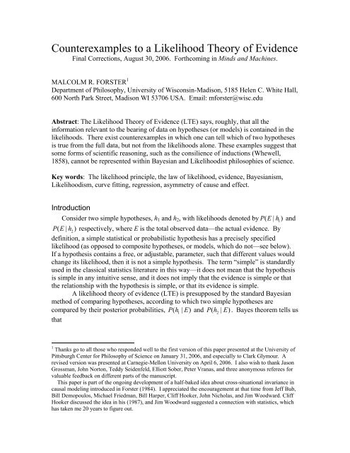
likelihoods? No, because the likelihoods are the same. So, this is a counterexample toLTE.In this example, the Backward hypothesis is derived from B 2by changing the storyabout how the exogenous variable is generated. If we were to replace this hypothesisinstead with a variant of B1, with the new story about how the exogenous values aregenerated, then the Backward and Forward hypotheses would be genuinelyindistinguishable on the basis of the full data—either one could have generated the data,and we couldn’t know from the data which is true. Yet, in this case, the Backwardhypothesis would have the higher likelihood! This does not contradict LTE because Ihave formulated it in a way that is completely neutral about how likelihoods are used.Nevertheless, it is a counterexample to the Law of Likelihood (Hacking 1965, Royall1997), which claims that evidence E supports A better than B or is stronger evidence forA than for B if and only if the likelihood of A is greater than the likelihood of B.Example 4: An interesting variation of Example 3 makes only one change.Instead of a list of x values that are distributed in a Gaussian way around a central value(x = 0), suppose that list comprising of two clusters—200 values distributed around x =−10 with an apparently Gaussian distribution, and a list of 200 x values centered around x= +10 with a similar distribution. The y values are generated in the same way as before.This is hypothesis F. The data, which are actually generated according to F, are shown inFig. 5. B is the false hypothesis that is analogous to that in Example 3, with the onlydifference being the obvious one, that the list of y values now form two clusters, onecentered at y = −10 and the other at y = +10. If we are given the full data, then we cantell that B is false by looking at the residuals, as before. So this is also a counterexampleto the Likelihood Theory of Evidence (LTE).Example 5: Example 4 is easilyturned into an example of modelcomparison. Construct the models Fand B by the ‘causal’ equationsY = α + βX + σUandX = a+ bY + sZ , respectively, where Uand Z are standard Gaussian, U isprobabilistically independent of X, andZ is independent of Y. F and B aremodels because the equations containadjustable parameters. The marginaldistributions for each trial are added inthe same way as in Example 4—theydon’t introduce any adjustableparameters, even though thedistributions vary from one trial to thenext (they are not identicallydistributed). F is true because one ofthe simple hypotheses in F is true:Suppose that the data are generated byY = X + U . This choice of1010115105-15 -10 -5 5 10 15-5-10-15yFigure 5: The asymmetry of regression. If aregression analysis is performed on the twoclusters of data separately, then the Forwardregression lines will coincide. But the Backwardregression lines are very distinct.x15

coefficients ensures that the variances of X and Y in the data are the same when the dataare clustered around X = −10 and X = +10, as shown in Fig. 5. With respect to the singleclustereddata (Fig. 3), the likelihood functions of models F and B are not equal. But,with respect to the data in Fig. 5, the maximum likelihoods of each model are now thesame, which means that the likelihood of any hypothesis in one model can be matched bythe likelihood of a hypothesis in the other model (see the Appendix for the proof). Inother words, the two models are equally good at accommodating the total data. But theyare predictively very different, as we are about to show.To complete the argument, we need only explain how the data (in Fig. 4) tell uswhich model is true. One way would be to show that every hypothesis in B is false byplotting the residuals, as explained in Example 2. But there is an easier way…The idea is to fit each model to the two clusters of data separately and comparethe independent estimates of the parameters obtained from the best fitting curves. I willdescribe this in a way that is reminiscent of the “test of hypotheses” that WilliamWhewell called the consilience of inductions (Whewell 1858, 1989). Let X1and Y1referto the cluster of data on the lower left of Fig. 5, while X2and Y2refer to the cluster onthe upper right. Then F can be rewritten in terms of two stochastic equations,Y1 = α1+ β1X1+ σU1, and Y2 = α2 + β2X2 + σU2, plus two constraints α1 = α2andβ1 = β2. 13 The two stochastic equations are not rival models; they are parts of the samemodel (let’s call them submodels). This way of writing the model makes no essentialchanges—it is just a different way of describing the same family of probabilitydistributions. If we fit the submodels to their respective clusters of data, we obtainindependent estimates of the parameters from the best fitting lines, which we can then useto test the constraints.The results will be as follows. Using the data in Fig. 5, the independentmeasurements of the F parameters will agree closely (by any statistical criterion). Butthe B model will fail the same test. To see this, rewrite B as X1 = a1+ bY1 1+ sV1, andX2= a2 + bY2 2+ sV2, plus the constraints a1 = a2and b1 = b2. The constraintb1= b 2will beverified, but the constraint a1 = a2is not close to being true. As shown in Fig. 5, theestimated values are approximately a1= − 10 and a2= + 10 . No statistical analysis canconclude that these are independent measurements of a single quantity. The data showsplainly that B is the false model, and therefore LTE is false.To put the point another way, B is false because it fails to predict features of onecluster of data from the rest of the data. When we fit B to the lower data cluster, we get abackwards regression curve that approximates the line Y = − 10 + 2X (the steep line onthe left in Fig. 5). Recall from Example 1, and Fig. 3, that this is the line from which Bcould have generated the lower data without us being able to tell. But we can tell that itdid not generate the upper cluster of data—because the line does not pass anywhere nearthe points in the upper right quadrant. B fails at this kind of cross-situational invariance(Forster, 1984), even though it is able to accommodate the full data perfectly well. The13 The word ‘constraint’ is borrowed from Sneed (1971), who introduced it as a way of constrainingsubmodels. Although the sense of ‘model’ assumed here is different from Sneed’s, the idea is the same.16

LTE fails because likelihood functions merely determine degrees of accommodation, notprediction.ConclusionThere are exceptions to the rule that all the empirical information relevant to thecomparison of hypotheses or models is contained in the likelihoods. Likelihoodmeasures how well a hypothesis is able to accommodate the data, but it leaves outimportant information about how well it can predict one part of the data from another.Very often, these predictive achievements are conveniently summarized in terms of theagreement of independent measurements of the theoretical quantities posited by themodels.The empirical overdetermination of parameters, or coefficients (Whewell 1958,Forster 1988), or constants (Norton 2000), played a pivotal role in Newton’s argumentfor universal gravitation (Whewell 1958, Forster 1988, Harper 2002), and in Perrin’sargument for the existence of atomic constituents of matter (see Norton 2000). That iswhy the Likelihood Theory of Evidence and the Bayesian philosophies of sciencefounded on it, will always fail to provide a complete theory of scientific reasoning.Statisticians have traditionally restricted their application of the LikelihoodTheory of Evidence to a narrower set of inferential problems—mainly, those involvingthe estimation of parameter values under the assumption that the model that defines themis true. But how does science establish the correctness of a model in the first place? Thatquestion calls for a deeper understanding of scientific reasoning than any version of thelikelihood theory can provide.In recent years, statisticians have turned their attention to the problem of modelcomparison, or model selection. Unfortunately, most of the proposed model selectioncriteria are based on the comparison of single numbers derived from the likelihoodfunction, and are therefore prone to the limitation described here. 14 Criteria such as AIC(Akaike 1973) and BIC (Schwarz 1978) are examples because they are based on themaximum likelihood, which is a feature of the likelihood function. Bayes Factorscompare average likelihoods derived directly from the likelihood function. 15Nevertheless, there is no reason why statistical methods cannot be used inevaluating the predictions of models, such as the predicted agreement of independentmeasurements; and this has always been a standard part of statistical practice. Theproblem is that theory lags practice. Future theories of statistical inference should paymore attention to well discussed ideas in philosophy of science, such as WilliamWhewell’s concept of scientific induction (which he calls the Colligation of Facts) andthe consilience of inductions (Whewell 1958, 1989). Glymour taps into many of thesame ideas in his early writings (e.g., Glymour 1980) and Forster (1988) uses14 Myrvold and Harper (2002) criticize the Akaike criterion of model selection (Forster and Sober 1994)because it underrates the importance of the agreement of independent measurements in Newton’s argumentfor universal gravitation (see Harper 2002 for an intriguing discussion of Newton’s argument). While thispaper supports their conclusion, it does so in a more precise and general way. The important advance inthis paper is (1) to point out that the limitation applies to all model selection criteria based on theLikelihood Principle and (2) to pinpoint exactly where the limitation lies. Nor is it my conclusion thatstatistics does not have the resources to address the problem.15 Wasserman (2000) provides a nice survey.17

Whewellian ideas in replying to arguments against the existence of forces. 16 A moregeneral theory of scientific reasoning may also connect with an old argument forscientific realism described by Earman (1978), and independently by Friedman (1981),both of which are discussed in Forster (1986). At the present time, these ideas have notbeen fully explored.Appendix10Theorem: If the maximum likelihood hypothesis in F is Y = X + U and the101observed variance of X is 101, then the observed variance of Y is also 101. Thus, the10maximum likelihood hypothesis in B is X = Y + Z , and they have the same101likelihood. Moreover, for any α, β, and σ, there exist values of a, b, and s such thatY = α + βX + σUand X = a+ bY + sZ have the same likelihood.Partial Proof: The observed X variance of data distributed in two Gaussian clusterswith unit variance centered at X = −10 and X = +10, where the observed means of X andY are 0, is equal to1 1 2 1 1 2VarX =2 N 2∑ xi+2 N 2∑ xj,where x idenotes X values in the lower cluster and x jdenotes X values in the upper cluster.If all the x iwhere equal to −10, and all the x jwere equal to +10, then VarX would beequal to 100. To that, one must add the effect of the local variances. More exactly,1 1 2 1 12VarX =2 N 2∑(( xi+ 10) − 10) +2 N 2∑ (( xj− 10) + 10) = 101.10100From the equationY = X + U , it follows that VarY =101101101+ 1 = 101. Standard10formulae for regression curves now prove that X = Y is the backwards regression line,101where the observed residual variance is also equal to 1. Therefore, the two hypotheseshave the same conditional likelihoods, and the same total likelihoods. It follows that the1010hypotheses Y = X + σUand X = Y + σ Z have the same likelihoods for any101101value of σ. It is also clear that for any α, β, and σ, there exist values of a, b, and s suchthat Y = α + βX + σUand X = a+ bY + sZ have the same likelihoods.ReferencesAitkin, M. (1991), “Posterior Bayes Factors,” Journal of the Royal Statistical Society B53: 111-142.Akaike, H. (1973), “Information Theory and an Extension of the Maximum LikelihoodPrinciple.” B. N. Petrov and F. Csaki (eds.), 2nd International Symposium onInformation Theory: 267-81. Budapest: Akademiai Kiado.Barnard, G. A. (1947), “Review of Wald’s ‘Sequential analysis’”, Journal of theAmerican Statistical Association, 42: 658-669.16 Hooker (1987) and Norton (1993, 2000) discuss relevant issues and examples; in fact, there is a wealth ofgood literature in the philosophy of and history of science that deserves serious attention from outsiders.18

Berger, James O. (1985), Statistical Decision Theory and Bayesian Analysis. SecondEdition, Springer-Verlag, New York.Berger, James O. and Wolpert, Robert L. (1988), The Likelihood Principle. 2nd edition.Hayward, California: Institute of Mathematical Statistics.Birnbaum, A. (1962), “On the Foundations of Statistical Inference (with discussion)”,Journal of the American Statistical Association 57: 269-326.Boik, Robert J. (2004), “Commentary”, in Mark Taper and Subhash Lele (eds), TheNature of Scientific Evidence, Chicago and London: University of Chicago Press,167-180.Burnham, Kenneth P. and Anderson, David R. (2002), Model Selection and Multi-ModelInference. New York: Springer Verlag.Earman, John (1978), “Fairy Tales vs. an Ongoing Story: Ramsey’s Neglected Argumentfor Scientific Realism.” Philosophical Studies 33: 195-202.Edwards, A. W. F. (1987), Likelihood. Expanded Edition. The John Hopkins UniversityPress: Baltimore and London.Fitelson, Branden (1999), “The Plurality of Bayesian Measures of Confirmation and theProblem of Measure Sensitivity,” Philosophy of Science 66: S362–78.Forster, Malcolm R. (1984), Probabilistic Causality and the Foundations of ModernScience. Ph.D. Thesis, University of Western Ontario.Forster, Malcolm R. (1986), “Unification and Scientific Realism Revisited.” In ArthurFine and Peter Machamer (eds.), PSA 1986. E. Lansing, Michigan: Philosophy ofScience Association. Volume 1: 394-405.Forster, Malcolm R. (1988), “Unification, Explanation, and the Composition of Causesin Newtonian Mechanics.” Studies in the History and Philosophy of Science 19:55 - 101.Forster, Malcolm R. (1988b), “Sober’s Principle of Common Cause and the Problem ofIncomplete Hypotheses.” Philosophy of Science 55: 538-59.Forster, Malcolm R. (2000), “Key Concepts in Model Selection: Performance andGeneralizability,” Journal of Mathematical Psychology 44: 205-231.Forster, Malcolm R. (forthcoming), “The Miraculous Consilience of QuantumMechanics,” in E. Eells and J. Fetzer (eds.) Probability in Science. Open Court.Forster, Malcolm R. and Elliott Sober (1994), “How to Tell when Simpler, MoreUnified, or Less Ad Hoc Theories will Provide More Accurate Predictions.”British Journal for the Philosophy of Science 45: 1 - 35.Forster, Malcolm R. and Elliott Sober (2004), ‘Why Likelihood?,’ in Mark Taper andSubhash Lele (eds), The Nature of Scientific Evidence, Chicago and London:University of Chicago Press, 153-165.Friedman, Michael (1981), “Theoretical Explanation,” in Time, Reduction and Reality.Edited by R. A. Healey. Cambridge: Cambridge University Press. Pages 1-16.19

Glymour, Clark (1980), “Explanations, Tests, Unity and Necessity.” Noûs 14: 31-50.Hacking, Ian (1965), Logic of Statistical Inference. Cambridge: Cambridge UniversityPress.Harper, William L. (2002), “Howard Stein on Isaac Newton: Beyond Hypotheses.” InDavid B. Malament (ed.) Reading Natural Philosophy: Essays in the History andPhilosophy of Science and Mathematics. Chicago and La Salle, Illinois: OpenCourt. 71-112.Hooker, Cliff A. (1987), A Realistic Theory of Science. Albany: State University of NewYork Press.Jeffreys, Harold (1961), Theory of probability. Third Edition. Oxford, The Clarendonpress.Mayo, Deborah G. (1996), Error and the Growth of Experimental Knowledge. Chicagoand London, The University of Chicago Press.Mermin, David N. (1990), “Quantum Mysteries Revisited.” American Journal of Physics,August 1990, pp.731-4.Myrvold, Wayne and William L. Harper (2002), “Model Selection, Simplicity, andScientific Inference”, Philosophy of Science 69: S135-S149.Norton, John D. (1993), “The Determination of Theory by Evidence: The Case forQuantum Discontinuity, 1900−1915”, Synthese 97: 1-31.Norton, John D. (2000), “How We Know about Electrons”, in Robert Nola and HowardSankey (eds.) After Popper, Kuhn and Feyerabend, Kluwer Academic Press, 67-97.Pearl, Judea (2000), Causality: Models, Reasoning, and Inference. Cambridge UniversityPress.Royall, Richard M. (1991), “Ethics and Statistics in Randomized Clinical Trials (withdiscussion),” Statistical Science 6: 52-88.Royall, Richard M. (1997), Statistical Evidence: A likelihood paradigm. Boca Raton:Chapman & Hall/CRC.Savage, L. J. (1976), “On rereading R. A. Fisher (with discussion)”, Annals of Statistics,42:441-500.Sakamoto, Y., M. Ishiguro, and G. Kitagawa (1986), Akaike Information CriterionStatistics. Dordrecht: Kluwer Academic Publishers.Schwarz, Gideon (1978), “Estimating the Dimension of a Model.” Annals of Statistics 6:461-5.Sneed, Joseph D. (1971), The Logical Structure of Mathematical Physics. Dordrecht: D.Reidel.Sober, Elliott (1993), “Epistemology for Empiricists.” In H. Wettstein (ed.), MidwestStudies in Philosophy. Notre Dame: University of Notre Dame Press; pp. 39-61.Wasserman, Larry (2000), “Bayesian model selection and model averaging.” Journal of20

Mathematical Psychology 44: 92-107.Whewell, William (1858), Novum Organon Renovatum, reprinted as Part II of the 3 rd thethird edition of The Philosophy of the Inductive Sciences, London, Cass, 1967.Whewell, William (1989), in Butts, Robert E. (ed.) Theory of Scientific Method. HackettPublishing Company, Indianapolis/Cambridge.Woodward, James. (2003), Making Things Happen: A Theory of Causal Explanation .Oxford and New York: Oxford University Press.21