Counterexamples to a Likelihood Theory of Evidence

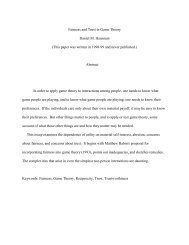
while h 2says that the probability of H is almost 0, say .0000001. Let M1be the beambalance model conjoined with h1, while M2is the beam balance model conjoined withh2. The simple hypotheses, h 1&( θ = 17) and h2 &( θ = 21) , for example, can be codedin the parameters by writing θ1= 17 and θ2= 21, respectively. It is now clear that thelikelihood functions for M1and M2are different despite the fact that the likelihoodfunctions for θ are equivalent for the purpose of estimating values of θ. This helpsblock a simple-minded argument against the Likelihood Principle, which goes somethinglike this: We can tell from the total evidence that M2is false because all simplehypotheses in M2assign a probability of almost 0 to the outcome H. But the two modelsare likelihood equivalent because their likelihood functions differ only by a constant.Agreed! This argument is wrong.This much seems clear: Most Bayesians, if not all, think that in order to gaininformation about which of two models is correct, it is at least necessary for there besome difference in the likelihood functions of the models. For if the likelihoods functionsof two models were exactly the same, the only way for the posterior probabilities to bedifferent would be for the priors to be different, but a difference in priors does not countas evidential discrimination. This is the assumption that I have referred to as theLikelihood Theory of Evidence (LTE).Preliminary ExamplesWhen a mass is hung on a spring, it oscillates for a period of time and comes to rest.After the system reaches an equilibrium state, the spring is stretched by a certain amount;let’s denote this variable by Y. To simplify the example, suppose that Y takes on adiscrete value 0 152, 2, 2, …, 2,2, because in-between positions are not stable. Maybe thisis because the motion of the device is constrained by a ball moving inside a lubricatedcylinder with a serrated surface (see Fig.2, right). The mass hung on the springconsists of a number of identical pellets(e.g., coins). This number is also anobserved quantity—denoted by X = 1, 2,3,…Conduct 2 trials of the experiment,and record the observations of (X, Y):Suppose they are (4,3.5) and (4,4.5).The data are represented by the soliddots in Fig. 2. Now consider thehypothesis A: Y = X + U, where U is aY7654321random error term that takes on values1 2 3 4 5 6−½ , or ½, each with probability ½.0XStrictly speaking, it’s a contradiction tosay that Y = 3.5 and then Y = 4.5 . Weshould introduce a different set ofvariables for each trial of theFigure 2: Discrete data, Section 4. The solid dotsare points at which data is observed, while theopen circles are points at which no data isobserved.7