ch 41.2.2-kadosh - Chemistry
ch 41.2.2-kadosh - Chemistry
ch 41.2.2-kadosh - Chemistry

You also want an ePaper? Increase the reach of your titles
YUMPU automatically turns print PDFs into web optimized ePapers that Google loves.
Thermal Effects in the Ultrafast Photoinduced Electron Transfer from a<br />
Molecular Donor An<strong>ch</strong>ored to a Semiconductor Acceptor<br />
WILLIAM STIER AND OLEG V. PREZHDO*<br />
Department of <strong>Chemistry</strong>, University of Washington, Seattle, Washington 98195-1700, USA<br />
(Received 12 November 2002 and in revised form 16 December 2002)<br />
Abstract. A nonadiabatic molecular dynamics (MD) simulation of the photoinduced<br />
electron transfer (ET) from a molecular electron donor to the TiO 2 semiconductor<br />
acceptor is carried out in a microcanonical ensemble with an average temperature<br />
of 350 K. The electronic structure of the dye–semiconductor system and the<br />
adiabatic dynamics are simulated by ab initio MD, while the nonadiabatic (NA)<br />
effects are incorporated by a quantum-classical mean-field approa<strong>ch</strong>. The ET dynamics<br />
are driven by thermal fluctuations that dominate ionic motions at the simulated<br />
temperature. The ground and excited state ion dynamics are similar; therefore,<br />
the <strong>ch</strong>ange in the quantum force due to the electronic photoexcitation can be<br />
neglected, and the final analysis is greatly simplified. The simulated ET occurs on a<br />
5-fs timescale, in agreement with recent ultrafast experimental data. Vibrational<br />
motions of the <strong>ch</strong>romophore ring carbons induce an oscillation of the photoexcited<br />
state energy, resulting in a bimodal distribution of the initial conditions for ET. At<br />
low energies the photoexcited state is localized primarily on the <strong>ch</strong>romophore, while<br />
at high energies the photoexcited state is substantially delocalized into the first 3<br />
surface layers of the TiO 2 surface. Thermally driven adiabatic transfer is the dominant<br />
ET me<strong>ch</strong>anism. Compared to the earlier simulation at 50 K, the rate of NA<br />
transfer at 350 K remains almost un<strong>ch</strong>anged, whereas the rate of adiabatic ET<br />
increases substantially.<br />
1. INTRODUCTION<br />
The dye-sensitized nanocrystalline solar cell, or<br />
Graetzel cell, is a promising alternative to the more<br />
costly traditional solar cell. 1–4 In a typical Graetzel cell, 5<br />
hot mobile electrons are generated within dye-sensitized<br />
titanium dioxide nanoparticles when photons are absorbed<br />
by the affixed <strong>ch</strong>romophore dye tuned to the<br />
desired wavelength. The nanoparticles or a highly porous<br />
nanocrystalline film are in contact with a transparent<br />
conducting glass electrode, by whi<strong>ch</strong> the excited<br />
electrons leave. The returning electrons are replenished<br />
to the dye from a mirrored conducting glass electrode<br />
through a mediating solution of iodide/triiodide.<br />
Considerable resear<strong>ch</strong> efforts have been focused on<br />
understanding the electron transfer (ET) dynamics of<br />
these cells, 5–36 with the goal of maximizing the photo-<br />
generated current, the voltage, and the photon-to-electron<br />
conversion yield. The overall photon-to-current efficiency<br />
is determined by a number of factors, most<br />
importantly the relative yields and rates of electron injection,<br />
recombination, and decay of the excited state of<br />
the dye. 8 A fast ET from the sensitizer dye to the semiconductor<br />
and a mu<strong>ch</strong> slower back ET are required.<br />
Low photovoltage appears to be a major limiting factor<br />
in the applications of the Graetzel cells. The experimentally<br />
observed photovoltage is below the theoretical<br />
maximum, likely due to the competition between ET<br />
and <strong>ch</strong>arge recombination pathways. 9 Knowledge of the<br />
rates and me<strong>ch</strong>anisms of these competing reactions is<br />
vital to the efficient improvement of the solar devices.<br />
*Author to whom correspondence should be addressed. E-mail:<br />
prezhdo@u.washington.edu<br />
Israel Journal of <strong>Chemistry</strong> Vol. 42 2002 pp. xx–xx
2<br />
The first step in the complex ET dynamics of the<br />
Graetzel cell is the ultrafast ET to the semiconductor<br />
from the atta<strong>ch</strong>ed molecular donor. The rate and me<strong>ch</strong>anism<br />
of this ultrafast ET are currently under active<br />
experimental 5,16–29 and theoretical 30–36 investigation. Recently,<br />
ET on a record femtosecond timescale has been<br />
reported. A femtosecond laser study of alizarin-sensitized<br />
TiO 2 revealed ET with a 6-fs injection time, 18 and a<br />
resonant photoemission study of bi-isonicotinic acidsensitized<br />
TiO 2-determined ET with an injection time of<br />
less than 3 fs. 25 Coherent oscillations in both the ET<br />
coordinate and the vibrational wave-packet motion of<br />
the ET product were seen under ultra-high vacuum<br />
(UHV). 6,28,29 No redistribution of the vibrational excitation<br />
energy can be expected at su<strong>ch</strong> ultrafast timescales, 6,28<br />
making it difficult to invoke the traditional Marcus–<br />
Levi<strong>ch</strong>–Jortner–Geris<strong>ch</strong>er 37–40 ET me<strong>ch</strong>anism, as well<br />
as the modern analytical and computational reaction rate<br />
theories. 30,41–49<br />
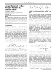
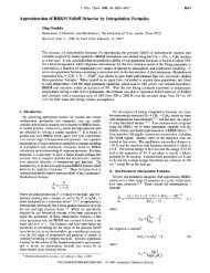
Two competing me<strong>ch</strong>anisms, whi<strong>ch</strong> can be differentiated<br />
as shown in Fig. 1, and whi<strong>ch</strong> require different<br />
conditions for optimum performance, have been proposed<br />
to explain the observed ultrafast ET between the<br />
dye and the semiconductor. 13,15 When the coupling is<br />
sufficient to induce a large splitting between the donor<br />
and acceptor state, so that the electron remains in the<br />
same adiabatic state as the system passes through the<br />
transition region, the me<strong>ch</strong>anism is adiabatic. In this<br />
case the ET occurs via redistribution of the electron<br />
density of the adiabatic state due to ionic motion, and<br />
the rate may be estimated using transition state<br />
theory. 50,51 If the coupling is sufficently small and the<br />
Fig. 1. Adiabatic and nonadiabatic pathways of electron transfer.<br />
In adiabatic ET (solid bold line) the electron remains in the<br />
same adiabatic state throughout the reaction, proceeding from<br />
the reactant state to the product state through the transition<br />
state. In nonadiabatic ET, the electron proceeds from the reactant<br />
state to the product state via a direct transition (bold dotted<br />
and dashed lines).<br />
Israel Journal of <strong>Chemistry</strong> 42 2002<br />
system passes through the transition region remaining in<br />
the same diabatic state and <strong>ch</strong>anging its adiabatic state,<br />
the ET is nonadiabatic (NA). NA ET occurs through a<br />
direct transition from the dye state to a manifold of<br />
acceptor states, and the rate could be calculated using<br />
standard Landau–Zener theory. 52 In experimental work<br />
the me<strong>ch</strong>anism must be deduced from observables su<strong>ch</strong><br />
as the reaction rate. For example, in cases where the<br />
Marcus theory of ET is applicable, the distinction between<br />
NA or adiabatic ET may be inferred from the rate<br />
equation<br />
(1)<br />
in whi<strong>ch</strong> the transmission factor κ should be approximately<br />
unity for adiabatic reactions and mu<strong>ch</strong> less than<br />
one for NA reactions. 50<br />
Whi<strong>ch</strong> me<strong>ch</strong>anism is at work is a practical concern<br />
because of design implications. NA transfer relies on a<br />
high density of states in the conduction band. Since the<br />
density of states increases with energy, 53 an increase of<br />
the <strong>ch</strong>romophore excited state energy relative to the<br />
edge of the conduction band will accelerate the transfer.<br />
At the same time, the photoexcitation energy and voltage<br />
will be lost due to the relaxation of the injected<br />
electron to the bottom of the conduction band. In the<br />
event of NA ET, it is also important to minimize <strong>ch</strong>romophore<br />
intramolecular vibrational relaxation, 54,55<br />
whi<strong>ch</strong> lowers the <strong>ch</strong>romophore energy and thereby the<br />
accessible density of conduction band states. NA ET is a<br />
purely quantum me<strong>ch</strong>anical process with many tunneling<br />
features. In particular, the rate of NA ET will decrease<br />
exponentially with increasing distance between<br />
the donor and acceptor species. Efficient NA ET requires<br />
short donor–acceptor bridges. Conversely, the<br />
adiabatic ET rate will be mu<strong>ch</strong> more weakly dependent<br />
on the density of acceptor states and will not exponentially<br />
decay with longer bridges. Since adiabatic transfer<br />
requires an energy fluctuation that can bring the system<br />
to the transition state, a fast ex<strong>ch</strong>ange of energy between<br />
vibrational modes of the <strong>ch</strong>romophore will increase the<br />
likelihood of adiabatic ET.<br />
Our first simulation of the ET was carried out at low<br />
temperature 34 to reflect UHV experimental conditions.<br />
6,28,29 The simulation revealed that the earliest ET<br />
was dominated by the NA me<strong>ch</strong>anism, with significant<br />
contributions from the adiabatic me<strong>ch</strong>anism at the later<br />
stages. It was found that the ET was localized to the first<br />
3 layers of the surface, with a single Ti atom closest to<br />
the <strong>ch</strong>romophore contributing over 20%. The simulation<br />
predicted a complex non-single-exponential time<br />
dependence of the ET process. In the current study, the
ET is investigated in the high temperature regime typical<br />
of the majority of experimental studies. 7–9,12–15,20–22<br />
2. THEORY<br />
The <strong>ch</strong>romophore–semiconductor system and simulation<br />
protocol adopted for NA MD are similar to those of<br />
our previous work, 34 apart from the following <strong>ch</strong>anges.<br />
The molecular electron donor an<strong>ch</strong>ored to the semiconductor<br />
acceptor is modified to provide a better description<br />
of the systems studied experimentally 7–9,12–17,22–24<br />
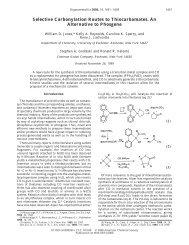
(Fig. 2a). A transition metal with a ligand (Fig. 2c) is<br />
added to the model <strong>ch</strong>romophore of our previous work<br />
(Fig. 2b). The ground electronic states of both the experimental<br />
<strong>ch</strong>romophore and the modified model are<br />
<strong>ch</strong>aracterized by a donor–acceptor interaction between<br />
the undivided n-electron pairs of ligands and d-orbitals<br />
of the transition metal, and the photoexcitation is now<br />
appropriately described by electron promotion from<br />
d-orbitals of the transition metal to the antibonding<br />
π*-orbital of the conjugated ring. The modified model is<br />
more appropriate for the ground state of the <strong>ch</strong>romophore,<br />
but does not <strong>ch</strong>ange the excited state, whose<br />
properties govern the ET between the molecule and the<br />
semiconductor. All three <strong>ch</strong>romophores in Fig. 2 have<br />
similar π* first excited states and, therefore, should<br />
show similar ET behavior. The difference between the<br />
Fig. 2. Chromophore molecules: (a) Chromophore used in<br />
experiments. 15 (b) Chromophore used in previous study. 34 (c)<br />
Chromophore used in this study. The <strong>ch</strong>romophore of the<br />
previous study was <strong>ch</strong>osen as an essential part of the experimental<br />
<strong>ch</strong>romophore. The current modification of the model<br />
<strong>ch</strong>romophore by addition of a d-electron metal and another<br />
ligand makes the ground electronic state of the n-electron<br />
donor d-orbital acceptor type similar to the experimental <strong>ch</strong>romophore.<br />
The photoexcited state is of the π*-type in all three<br />
molecules.<br />
model <strong>ch</strong>romophore in Fig. 2 and those typically used is<br />
less than the difference between the two <strong>ch</strong>romophores<br />
for whi<strong>ch</strong> ultrafast ET has been observed on this<br />
timescale. 18,25<br />
Experiments for a variety of systems 15,18,28,56–62 have<br />
been carried out at temperatures ranging from UHV to<br />
ambient temperatures and above, with the majority of<br />
data available for room temperature. The low temperature<br />
UHV case was considered previously. 34 The high<br />
temperature case is investigated in this work. The temperature<br />
of the microcanonical simulation reported here<br />
averages around 350 K, with a 10-K fluctuation around<br />
the average.<br />
It has been found in the high temperature simulation<br />
that the ET dynamics are dominated by random thermal<br />
fluctuations of ions, whi<strong>ch</strong> are similar in both the<br />
ground and excited electronic states. A directional electronic<br />
force is generally expected to act on ions once the<br />
equilibrated ground state is photoexcited. The force appears<br />
when the minima in the potential energy surfaces<br />
of the ground and excited electronic states are displaced<br />
in ionic coordinates. Ions initially located in the minimum<br />
of the ground electronic state find themselves on a<br />
slope of the excited electronic state surface. It has been<br />
found that the amplitude of thermal motion of ions at<br />
350 K exceeds the displacement between the ground<br />
and excited state minima. The <strong>ch</strong>ange due to photoexcitation<br />
in the electronic force acting on ions is small.<br />
Its contribution to ion dynamics can be neglected relative<br />
to thermal motions. This observation greatly simplifies<br />
the calculation. Under the assumption that the<br />
ground and excited state dynamics are similar, an ensemble<br />
of independent NA MD trajectories is not required,<br />
as it is in the traditional approa<strong>ch</strong>es. 63–82 The<br />
input to NA MD can be obtained from a ground state<br />
trajectory as described below.<br />
The simulation cell consists of a <strong>ch</strong>romophore molecule<br />
bonded to a semiconductor surface. The surface is<br />
composed of a slab of rutile five layers thick, terminated<br />
on both sides with hydrogen and hydroxyl groups as<br />
would be expected if the surface were exposed to ambient<br />
humidity. The bottom two layers of the slab are<br />
frozen in the bulk configuration. A sufficiently large<br />
vacuum layer is added to the simulation cell to insure<br />
that the top of one slab does not interact with the bottom<br />
of the next slab within the infinite array of slabs. The<br />
<strong>ch</strong>romophore molecule consists of an isonicotinic acid<br />
molecule with a silver ion bonded to the lone pair of the<br />
nitrogen, and a cyanide ion bonded to the opposite side<br />
of the silver. The <strong>ch</strong>romophore is atta<strong>ch</strong>ed to the surface<br />
by a dehydrogenation reaction.<br />
The electronic structure of the combined <strong>ch</strong>romophore–semiconductor<br />
system is obtained by density-<br />
Stier and Prezhdo / Thermal Effects in Photoinduced Electron Transfer<br />
3
Au: Wang<br />
is not in ref<br />
87?<br />
4<br />
functional theory (DFT) with the VASP code. 83–85 The<br />
periodic boundary conditions and plane wave basis sets<br />
of the VASP code are especially effective for extended<br />
periodic systems su<strong>ch</strong> as semiconductors. The core<br />
electrons are simulated using the Vanderbilt pseudopotentials,<br />
86 and only the valence electrons are treated<br />
explicitly. The generalized gradient functional due to<br />
Perdew and Wang 87 is used. The energy cutoff for the<br />
plane wave basis was 202.7 eV, yielding a basis set of<br />
approximately 112,000 plane waves. The Kohn–Sham<br />
orbitals are constructed from the plane wave basis set<br />
and are used to describe the electronic states of the<br />
system.<br />
The assembled structure of the dye on the TiO 2 surface<br />
is brought to equilibrium at the temperature of<br />
350 K. A 1 fs MD timestep is used. Upon equilibration,<br />
a 1-ps adiabatic ground state MD trajectory is run in the<br />
microcanonical ensemble. This is the production run for<br />
NA MD.<br />
Under the assumption that the ET dynamics are<br />
dominated by thermal fluctuations of ions, su<strong>ch</strong> that ion<br />
dynamics are similar in the ground and excited electronic<br />
states, only the ground state trajectory data are<br />
needed to perform NA MD. For ea<strong>ch</strong> of the 1000 steps<br />
of the 1-ps production run, adiabatic energies and NA<br />
couplings are determined. In the one-electron picture,<br />
the adiabatic energies ε i are given by the energies of the<br />
Kohn–Sham orbitals. The NA couplings d ij are calculated<br />
numerically 66 based on the overlap of the Kohn–<br />
Sham orbitals φ i at sequential timesteps<br />
Israel Journal of <strong>Chemistry</strong> 42 2002<br />
(2)<br />
The adiabatic energies and NA couplings define the<br />
diagonal and off-diagonal elements of the electronic NA<br />
Hamiltonian, correspondingly<br />
(3)<br />
The NA Hamiltonian is time-dependent through the<br />
time-dependence of the locations of ions R.<br />
100 configurations are harvested from the first 900 fs<br />
of the 1-ps production run to use as initial configurations<br />
of the system at the time the photon is absorbed. For<br />
ea<strong>ch</strong> configuration, the Kohn–Sham orbital corresponding<br />
to the <strong>ch</strong>romophore first excited state is determined.<br />
An electron is promoted from an occupied orbital to the<br />
excited state orbital to initiate a NA MD run. The NA<br />
dynamics are carried out in the one-electron approximation<br />
(4)<br />
by propagating the occupations c i of 26 excited states<br />
using the NA Hamiltonian specified above. The state<br />
occupations are propagated by the second-order<br />
differencing s<strong>ch</strong>eme 88<br />
(5)<br />
with a timestep of 10 –3 fs.<br />
The extent of ET is determined by the fraction of the<br />
excited state electron that has left the dye. The density<br />
generated by the one-electron excited state wave function<br />
Ψ is integrated over the region of space occupied by<br />
the dye<br />
(6)<br />
and followed as a function of time. In order to establish<br />
the ET me<strong>ch</strong>anism, the evolution of the electron density<br />
is decomposed into nonadiabatic and adiabatic contributions.<br />
(7)<br />
The first term is the NA ET, whi<strong>ch</strong> arises from<br />
<strong>ch</strong>anges in the excited electron’s occupation of the adiabatic<br />
states. The second term is due to <strong>ch</strong>anges in orbital<br />
localizations and gives adiabatic transfer 34 (Fig. 1).<br />
3. RESULTS<br />
The evolution of the excited state energies of the combined<br />
dye–semiconductor system during the 1-ps production<br />
run is plotted in Fig. 3a. The majority of the<br />
states are bulk and surface states representing the conduction<br />
band of the semiconductor. Only one excited<br />
state of the dye, indicated by the bold line, falls within<br />
the energy range shown in Fig. 3a. This state is occupied<br />
at the beginning of a NA run. As can be clearly seen in<br />
the figure, the energy of the dye state oscillates as a<br />
function of time. The amplitude of the oscillation is<br />
several tenths of an electronvolt. The oscillation is relatively<br />
small compared to the several-electronvolt excita-
Au: Is the<br />
fuzziness in<br />
(a) part of<br />
the data, or<br />
should the<br />
background<br />
be cleaned<br />
up?<br />
(a) (b)<br />
(c) (d)<br />
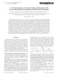
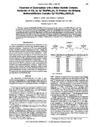
Fig. 3. (a) Time evolution of the <strong>ch</strong>romophore excited state (dark line) relative to the conduction band of TiO 2. The fluctuation of<br />
the <strong>ch</strong>romophore excited state energy by fractions of eV is relatively small compared to the excitation energy of several eV, but<br />
has a dramatic effect on the positioning of the <strong>ch</strong>romophore state in the TiO 2 conduction band. (b) Autocorrelation function of<br />
the <strong>ch</strong>romophore excited state energy of part a. Within 10 fs the correlation function decreases to half of its original value. The<br />
subsequent oscillation persists for the time of the simulation and indicates that the evolution of the excited state energy is highly<br />
correlated. (c) Fourier transform of autocorrelation function of part (b). The persistent oscillation of the <strong>ch</strong>romophore excited<br />
state energy is dominated by a 1600 cm –1 mode. (d) Fourier transforms of the ion velocity autocorrelation functions. The insert<br />
shows the <strong>ch</strong>romophore part of the system, Fig. 2, with the atoms represented by the data symbols. Circles represent atoms that<br />
show no oscillation frequencies within the range of the plot. Only the carbon and nitrogen atoms of the molecule oscillate at 1600<br />
cm –1 . The evolution of the <strong>ch</strong>romophore excited state seen in part (a) is due to the C–C-stret<strong>ch</strong>ing mode of the <strong>ch</strong>romophore.<br />
tion energy of the dye, but has a substantial impact on<br />
positioning of the dye state in the conduction band of<br />
TiO 2. The density of states of the conduction band increases<br />
with energy, 53 su<strong>ch</strong> that an excited state of the<br />
dye near the oscillation minimum can interact with substantially<br />
fewer semiconductor states than a high energy<br />
dye state.<br />
The autocorrelation function<br />
(8)<br />
of the dye state energy E(t) averaged over the production<br />
trajectory is given in Fig. 3b. The autocorrelation<br />
function <strong>ch</strong>aracterizes how long the excited state of the<br />
dye keeps memory of its past evolution. 89 The autocorrelation<br />
function of a perfectly periodic motion oscillates,<br />
rea<strong>ch</strong>ing its initial value at every oscillation, whereas<br />
the autocorrelation function of a random motion decays<br />
to zero. The autocorrelation function shown in Fig. 3b<br />
rapidly decays to about a third of its initial value, but<br />
then continues a regular oscillation for the duration of<br />
the production run. The persistent oscillation of the<br />
Stier and Prezhdo / Thermal Effects in Photoinduced Electron Transfer<br />
5
6<br />
autocorrelation function with a substantial amplitude is<br />
indicative of a correlated evolution of the dye excited<br />
state. The Fourier transform of the autocorrelation function<br />
shown in Fig. 3c peaks at 1600 cm –1 . This frequency<br />
is within the range associated with a carbon stret<strong>ch</strong>,<br />
immediately revealing the origin of the oscillation.<br />
Since the first excited state of the <strong>ch</strong>romophore is a<br />
π-state localized on the ring carbons, an oscillation of<br />
the ring carbons should modulate the energy of the state.<br />
In order to establish the types of ion motions available<br />
at the 1600 cm –1 frequency, Fourier transforms of<br />
velocity autocorrelation functions of all atoms in the<br />
combined system have been computed. The result is<br />
shown in Fig. 3d on a logarithmic scale. Only <strong>ch</strong>romophore<br />
carbon and nitrogen atoms exhibit motions with<br />
frequencies near 1600 cm –1 , with the peak at 1600 cm –1<br />
dominated by the three middle carbons. The first excited<br />
state of the dye is localized on the four middle carbons:<br />
The persistent oscillation of the dye excited state energy<br />
shown in Fig. 3a is indeed due to a C–C-stret<strong>ch</strong>ing<br />
mode.<br />
In the combined dye–TiO 2 system, the dye excited<br />
state interacts with the TiO 2 conduction band. As a<br />
result, the adiabatic states represented in the one-electron<br />
picture by the Kohn–Sham orbitals of the combined<br />
system are, generally, delocalized between the <strong>ch</strong>romophore<br />
and the semiconductor. It is assumed in the<br />
current simulation that photoexcitation promotes an<br />
electron into the adiabatic state with the largest localization<br />
on the dye. This is expected with strong excited<br />
state selection rules with transition dipole moments<br />
favoring excitation of the dye fragment, or with relatively<br />
long laser pulses that by the time–energy uncertainty<br />
relationship can select a state with a stationary,<br />
adiabatic state of a given energy. The opposite limit is<br />
the diabatic excitation, where the laser excites a superposition<br />
of adiabatic states that best corresponds to the<br />
dye excited state in the absence of a semiconductor. The<br />
details of the photoexcitation realized in experiments<br />
depend on both properties of the dye–semiconductor<br />
system, su<strong>ch</strong> as transition dipole moments between<br />
ground and excited states, and properties of the laser<br />
pulse, su<strong>ch</strong> as its shape, duration, and polarization. Investigation<br />
of the photoexcitation details extends beyond<br />
the scope of the present study, whi<strong>ch</strong> takes the<br />
adiabatic excitation limit. Figure 4a shows localization<br />
L p of the photoexcited state φ p<br />
Israel Journal of <strong>Chemistry</strong> 42 2002<br />
(9)<br />
on the <strong>ch</strong>romophore along the production run. The<br />
photoexcited state is defined in the adiabatic limit as the<br />
state with the largest localization on the dye, <strong>ch</strong>osen<br />
within a range of states of the combined system at the<br />
energies corresponding to the excited state energy of the<br />
isolated <strong>ch</strong>romophore, Fig. 2c. The degree to whi<strong>ch</strong> the<br />
photoexcited state is localized on the dye varies substantially<br />
along the trajectory. In many instances the<br />
photoexcited state is localized on the dye 80% or more,<br />
similar to our previous low temperature simulation. 34<br />
Very often, the photoexcited state is less than 50%<br />
localized on the dye. In su<strong>ch</strong> cases, the excited state of<br />
the isolated <strong>ch</strong>romophore, the diabatic state, contributes<br />
to several, typically 2 or 3, adiabatic states of the combined<br />
system; see Fig. 5a below.<br />
A closer look at the data of Figs. 3a and 4a reveals<br />
that the localization of the photoexcited state on the dye<br />
has the same fluctuation as the energy of the photoexcited<br />
state. The autocorrelation function<br />
(10)<br />
of the localization of the initial state, Fig. 4b, and its<br />
Fourier transform, Fig. 4c, are very similar to those of<br />
the state energy, Figs. 3b and 3c. The localization oscillates<br />
with the same frequency as the energy. This result<br />
can be expected, since the density of states in the conduction<br />
band grows with energy, Fig. 5b, increasing the<br />
likelihood of interaction and mixing between the dye<br />
and semiconductor states. The localization varies with<br />
energy, and thereby oscillates with the same frequency<br />
as the energy.<br />
The correlation between the energy of the photoexcited<br />
state and its localization on the <strong>ch</strong>romophore<br />
fragment is illustrated in Fig. 4d, whi<strong>ch</strong> shows the data<br />
for the 100 randomly <strong>ch</strong>osen initial conditions. The<br />
correlation is far from perfect; however, a general trend<br />
can be seen very clearly. A higher density of semiconductor<br />
states does not always imply that more states will<br />
be coupled to the dye excited state. The coupling relies<br />
not only on energy resonance, but also on other <strong>ch</strong>aracteristics<br />
of semiconductor states, su<strong>ch</strong> as their localization<br />
at the surface. Fluctuations in the surface structure<br />
cause <strong>ch</strong>anges in the localization and coupling. The<br />
effect of fluctuations in the surface structure is further<br />
emphasized by a finite depth of the TiO 2 slab. The<br />
simulation represents the conduction band continuum<br />
by a finite number of states. Consequently, the coupling<br />
and mixing of the dye excited state with the surface and<br />
bulk states of the substrate is more discretized than it<br />
may be in reality. Although there will be on average a<br />
greater amount of mixing and coupling when the energy<br />
of the dye excited state is high, there will always be<br />
cases where the mixing and localization are more or less
(a) (b)<br />
(c) (d)<br />
Fig. 4. (a) Time evolution of localization of the photoexcited state of the <strong>ch</strong>romophore–TiO 2 system on the <strong>ch</strong>romophore<br />
fragment. Due to coupling to the TiO 2 conduction band, the <strong>ch</strong>romophore excited state is onto the semiconductor. The<br />
delocalization is stronger, with more TiO 2 states coupled to the <strong>ch</strong>romophore state. Since the density of the conduction band<br />
states increases with energy, the <strong>ch</strong>romophore localization of the photoexcited state decreases with increasing energy. (b)<br />
Autocorrelation function of the time evolution of localization from part (a). Similarly to the energy of the photoexcited state, Fig.<br />
3, the localization of the photoexcited state evolves with a persistent memory. (c) Fourier transform of the autocorrelation<br />
function of part (b). The localization of the photoexcited state on the <strong>ch</strong>romophore fragment oscillates with the same frequency<br />
as the energy of the photoexcited state, Fig. 3. (d) Chromophore localization of the excited state plotted against the state energy.<br />
There is a greater density of TiO 2 states at higher energies, leading to a stronger coupling and a larger delocalization of the<br />
<strong>ch</strong>romophore state.<br />
than the amount predicted by the line associated with the<br />
average. It is this factor that causes the random spread of<br />
the data points from the linear fit.<br />
At low energies, the first excited state of a bare<br />
<strong>ch</strong>romophore directly corresponds to a single state of<br />
the combined <strong>ch</strong>romophore–semiconductor system.<br />
This is illustrated in Fig. 5a whi<strong>ch</strong> shows the energy<br />
dependence of the number of adiabatic states of the<br />
combined <strong>ch</strong>romophore–semiconductor system that are<br />
substantially localized on the <strong>ch</strong>romophore. At low energies<br />
there is only one su<strong>ch</strong> state. As the energy increases,<br />
the diabatic state of the bare <strong>ch</strong>romophore inter-<br />
acts and mixes with several semiconductor states. At<br />
high energies, three adiabatic states of the <strong>ch</strong>romophore–<br />
semiconductor system can have substantial contributions<br />
from the <strong>ch</strong>romophore excited state. This implies<br />
that in the diabatic limit, where the initial photoexcitation<br />
is localized solely on the <strong>ch</strong>romophore, a superposition of<br />
three adiabatic <strong>ch</strong>romophore–semiconductor states will<br />
be required to represent the initial condition for ET in<br />
the NA dynamics simulation. It is quite interesting that<br />
the number of the semiconductor states that couple and<br />
mix with the <strong>ch</strong>romophore state saturates around three<br />
at high energies. While the density of semiconductor<br />
Stier and Prezhdo / Thermal Effects in Photoinduced Electron Transfer<br />
7<br />
Au: correct<br />
word?
8<br />
(a) (b)<br />
Fig. 5. (a) Energy dependence of the number of adiabatic states of the <strong>ch</strong>romophore–semiconductor system that have a 10% or<br />
more contribution from the <strong>ch</strong>romophore state. At low energies the first excited state of a bare <strong>ch</strong>romophore directly corresponds<br />
to a single state of the combined <strong>ch</strong>romophore–semiconductor system. The density of states in the TiO 2 conduction band<br />
increases with energy, increasing the likelihood of mixing of the <strong>ch</strong>romophore state with semiconductor states. At higher<br />
energies the average number of semiconductor states that couple and mix with the <strong>ch</strong>romophore state saturates around 3. (b) The<br />
density of states of the system as derived from the adiabatic MD. Within the range of energies observed for the donor state the<br />
density of conduction band states increases steadily. Inset—the density of states of the system including the valence and<br />
conduction bands. Peaks corresponding to ground state of the dye and surface states can be seen slightly above the bulk valence<br />
band. States were compiled from gamma point energies over the 1000 fs of the MD run, vice the normal compilation of k-point<br />
energies at equilibrium geometry.<br />
states, Fig. 5b, continues to increase with energy, the<br />
number of surface states that couple to the <strong>ch</strong>romophore<br />
state, Fig. 5a, rea<strong>ch</strong>es a threshold at –5.5 eV.<br />
The oscillation of the photoexcited state energy,<br />
Fig. 3a, results in a bimodal energy distribution peaked<br />
around the turning points of the oscillation. This distribution<br />
of the photoexcited state energy is shown in<br />
Fig. 6. The high energy turning point of the oscillation<br />
of the photoexcited state energy corresponds to shortening<br />
of the C–C distance of the carbon-stret<strong>ch</strong>ing motion<br />
Fig. 6. Distribution of the photoexcited state energies. The two<br />
peaks correspond to the low and high energy turning points of<br />
the oscillating excited state energy, Fig. 3a.<br />
Israel Journal of <strong>Chemistry</strong> 42 2002<br />
at 1600 cm –1 , Fig. 3d. The photoexcited state is dominated<br />
by the antibonding π*-orbital. The shortening of<br />
the C–C distance increases the interaction between the<br />
Pz electrons of the carbon atoms, and as a result, the<br />
splitting between the π-bonding and π*-antibonding orbitals<br />
becomes larger, and the energy of the π* excited<br />
state increases. On the other hand, elongation of the<br />
C–C distance diminishes the interaction between the Pz electrons of the carbon atoms, resulting in a smaller<br />
splitting and a lower excited state energy.<br />
The existence of the bimodal distribution of the<br />
photoexcited state energy that depends on instantaneous<br />
positions of ions encourages examination of the ET<br />
behavior for the low and high energy initial conditions.<br />
The time evolution of the ET coordinate averaged over<br />
the low and high energy initial conditions is shown in<br />
Figs. 7a and 7b, respectively. The average overall initial<br />
conditions are given in Fig. 7c. The simulation results<br />
depicted by circles are fitted by the exponential<br />
ET = 1 – exp [(t + t ) / τ] (11)<br />
0<br />
where τ is the ET timescale. The fit, shown by a solid<br />
line, takes into account the fact that a partial ET has<br />
already occurred due to photoexcitation, prior to the<br />
simulated excited state dynamics. Due to the<br />
photoexcitation contribution to ET, the ET coordinate at<br />
time t = 0 starts at ET t = 0 = 1 – exp (t 0/τ) rather than at 0.<br />
t 0 represents the time the system is advanced along the<br />
?
(a) (b)<br />
(c)<br />
ET reaction coordinate by the photoexcitation. The<br />
adiabatic and NA contributions to ET are shown in<br />
Fig. 7 by triangles and diamonds, correspondingly.<br />
Since the adiabatic and NA me<strong>ch</strong>anisms are not defined<br />
for the photoexcitation contribution to ET, the adiabatic<br />
and NA contributions to ET are plotted starting at zero<br />
and are fitted by<br />
ET = C [1 – exp (t/τ)] (12)<br />
shown by solid lines. The photoexcitation contribution<br />
to ET, the ETt = 0 constant, together with the adiabatic<br />
and NA contributions, add up to the total electron transfer<br />
coordinate of eq 11. It follows, then, that Cadiab. +<br />
CNA + ETt = 0 = 1.<br />
The temperature increase from 50 K in our previous<br />
simulation to 350 K in the current study has a significant<br />
effect on the ET timescale, whi<strong>ch</strong> decreased from about<br />
30 fs at 50 K to 5 fs at 350 K, Fig. 7c. The simulated 5-fs<br />
timescale of ET between the isonicotinic acid and TiO2 agrees with the ET from bi-isonicotinic acid to TiO2 surface reported to occur in less than 3 fs, 25 as well as<br />
with the 6-fs ET time observed at room temperature<br />
between the alizarin <strong>ch</strong>romophore and TiO2 surface. 18 In<br />
all cases the electron donors are directly atta<strong>ch</strong>ed to the<br />
Fig. 7. (a) Time evolution of the ET coordinate, circles, averaged<br />
over the low energy initial conditions corresponding to<br />
the left peak of the bimodal distribution of the photoexcited<br />
state energy, Fig. 6. The adiabatic and NA contributions to ET<br />
are shown by triangles and diamonds, correspondingly. The<br />
evolution of the total ET is fitted with eq 11. The fit takes into<br />
account the fact that a partial ET has already occurred due to<br />
photoexcitation and prior to the simulated excited state dynamics.<br />
The evolutions of the adiabatic and NA contributions<br />
to ET are fitted with eq 12. (b) Same as part a, but averaged<br />
over the high energy initial conditions represented by the right<br />
peak of the bimodal distribution of Fig. 6. (c) Same as part a,<br />
but averaged over all initial conditions.<br />
electron acceptors without any kind of bridge, leading to<br />
one of the fastest ET events.<br />
The excited state ET dynamics start with over 50% of<br />
the electron pre-transferred by the photoexcitation. The<br />
adiabatic ET me<strong>ch</strong>anism, whi<strong>ch</strong> relies on thermal fluctuations<br />
driving the system over the transition state,<br />
becomes mu<strong>ch</strong> more efficient at the increased temperature,<br />
and predominates over the NA me<strong>ch</strong>anism. Adiabatic<br />
transfer is both faster and has a larger contribution<br />
to the overall transfer. This is in contrast to the low<br />
temperature simulation, 34 where the NA ET me<strong>ch</strong>anism<br />
is more prominent than the adiabatic me<strong>ch</strong>anism. The<br />
rate of the low energy NA transfer is almost un<strong>ch</strong>anged<br />
from 50 to 350 K, whereas the rate of adiabatic ET<br />
increased dramatically.<br />
The ET events originating with low and high energies,<br />
Figs. 7a and 7b, corresponding to the low and high<br />
energy parts of the bimodal distribution of initial conditions,<br />
Fig. 6, differ substantially. The high energy transfer<br />
is three times faster than the low energy transfer. The<br />
largest difference can be seen in the timescales and<br />
amplitudes of NA ET. The NA ET timescale determined<br />
here with the low energy initial conditions corresponds<br />
quantitatively to the NA ET time obtained in the 50 K<br />
Stier and Prezhdo / Thermal Effects in Photoinduced Electron Transfer<br />
9
10<br />
simulation of ref 34. The NA transfer becomes significantly<br />
faster with a higher initial energy due to access to<br />
a larger density of TiO 2 states. However its contribution<br />
to the total ET is diminished, and the adiabatic me<strong>ch</strong>anism<br />
completely predominates over the NA me<strong>ch</strong>anism<br />
at high initial energies. The adiabatic and NA contributions<br />
are comparable at low energies. Pre-ET by<br />
photoexcitation is more important at higher energies<br />
and is less pronounced at lower energies, where the<br />
excited state dynamics plays a major role. Assuming<br />
that photoexcitation places the system in an adiabatic<br />
excited state, about 50% of ET occurs due to photoexcitation<br />
and 50% by excited state dynamics (Fig. 7c).<br />
4. DISCUSSION AND CONCLUSIONS<br />
The simulated photoinduced ET between the molecular<br />
electron donor and the TiO 2 acceptor typical of the dyesensitized<br />
semiconductor nanomaterials used in solar<br />
cells, photocatalysis, and photoelectrolysis applications<br />
is thermally driven at 350 K. Pronounced thermal effects<br />
are evident both in the equilibrium ground state<br />
fluctuations that define the distribution of initial conditions<br />
for ET, and in the nonequilibrium excited state ET<br />
dynamics that are dominated by the thermally activated<br />
adiabatic me<strong>ch</strong>anism. The rate of NA transfer is nearly<br />
un<strong>ch</strong>anged from 50 to 350 K, while the adiabatic ET rate<br />
is dramatically increased.<br />
A detailed picture of the ET process follows from the<br />
simulation. As should be expected, higher temperatures<br />
increase the likelihood of a fluctuation that can drive the<br />
ET coordinate over the transition state. The adiabatic ET<br />
is thereby enhanced at high temperatures, becoming<br />
mu<strong>ch</strong> more effective than the NA, predominating both<br />
in magnitude and timescale.<br />
Another, more subtle, effect is also induced by the<br />
thermal fluctuations. Since the photoexcited state is a<br />
π*-state localized on <strong>ch</strong>romophore carbons, thermal<br />
motions of the carbon atoms <strong>ch</strong>ange the energy of the<br />
state. Although the energy variation is only a fraction of<br />
an electronvolt, whi<strong>ch</strong> is small relative to the photoexcitation<br />
scale of several electronvolts, it has a significant<br />
impact on the ET process. Since the density of the<br />
semiconductor states increases with energy, the higher<br />
the energy of the electron donor, the more likely it will<br />
interact with an acceptor state. The oscillation of the<br />
photoexcited state energy slows down at the high and<br />
low energy turning points, and the energies tend to<br />
cluster around these points, resulting in a bimodal distribution<br />
of the initial conditions.<br />
The two distinct types of initial conditions observed<br />
in the simulation are responsible for two kinds of ET<br />
events. At lower initial energies the photoexcited state is<br />
localized primarily on the <strong>ch</strong>romophore, and the ET is<br />
Israel Journal of <strong>Chemistry</strong> 42 2002<br />
largely determined by the excited state dynamics. At<br />
higher initial energies a significant fraction of the ET<br />
has already occurred upon photoexcitation. The photoexcited<br />
state is significantly delocalized onto the semiconductor,<br />
and the excited state dynamics are responsible<br />
for only the last third of the ET. These conclusions<br />
are based on the adiabatic photoexcitation model, where<br />
it is assumed that the laser prepares the combined <strong>ch</strong>romophore–semiconductor<br />
system in an adiabatic excited<br />
state. A diabatic photoexcitation model provides the<br />
opposite limit, where the initial photoexcitation is assumed<br />
fully localized on the <strong>ch</strong>romophore, spanning 2<br />
or 3 adiabatic states. A more detailed analysis of the<br />
interaction between the system and the laser field is<br />
required in a general case.<br />
The ET in question has been proposed to be either an<br />
adiabatic ET in whi<strong>ch</strong> the donor state is strongly coupled<br />
to a single acceptor state, or a NA process in whi<strong>ch</strong> the<br />
donor state is weakly coupled to a manifold of acceptor<br />
states (Fig. 1). One may postulate that the reaction coordinate<br />
is an activationless NA direct transition from the dye<br />
state to a continuum of conduction band states. In this<br />
case, the Fermi golden rule would give an estimate of the<br />
reaction rate. If, however, the ET was an adiabatic transfer<br />
between the dye state to a particular conduction band state,<br />
a Marcus theory of ET would be more appropriate (eq 1).<br />
Relatively few (1–3) states of the conduction band initially<br />
couple to the excited state of the <strong>ch</strong>romophore. Often,<br />
especially with the low energy part of distribution of the<br />
<strong>ch</strong>romophore state energies, the acceptor states are higher<br />
in energy than the donor state, su<strong>ch</strong> that an activation is<br />
needed. Both activated ET and activationless direct relaxation<br />
are observed in this study.<br />
The timescales and dominant me<strong>ch</strong>anisms of ET<br />
vary, depending on whether the initial state has high or<br />
low energy. At high initial energies ET is extremely fast<br />
and purely adiabatic. At low initial energies barriers to<br />
ET arise, and the contribution of the NA me<strong>ch</strong>anism<br />
approa<strong>ch</strong>es that of the adiabatic me<strong>ch</strong>anism. The timescale<br />
of ET by the NA me<strong>ch</strong>anism mat<strong>ch</strong>es the NA ET<br />
timescale of the low temperature simulation. 34 The large<br />
differences seen in the features of the ET processes<br />
occurring at low (50 K, ref 34) and high (350 K, this<br />
paper) temperatures suggest that a systematic study of<br />
the ET process over the whole temperature range can<br />
produce a Marcus theory description of ET, eq 1, with<br />
adiabatic activation energy, NA transmission factor κ,<br />
and turnover between a quantum NA tunneling regime<br />
and a thermally activated adiabatic ET regime.<br />
For the system under study, ET occurs on a 5-fs<br />
timescale. This is in agreement with the ultrafast experimental<br />
data for the alizarin 18 and bi-isonicotinic acid 25<br />
<strong>ch</strong>romophores that, similarly to our model, are directly
Au: What is<br />
PRF?<br />
connected to the semiconductor. In other cases, where<br />
one or more bridging groups are connecting <strong>ch</strong>romophores<br />
to TiO 2, the ET timescale is at least an order<br />
of magnitude slower. 14,15,28,29,33<br />
The coupling of the ET process to stret<strong>ch</strong>ing vibrations<br />
of carbon atoms of the conjugated <strong>ch</strong>romophore<br />
seen in the present simulation has been observed by a<br />
direct measurement with the perylene <strong>ch</strong>romophore. 28,29<br />
The vibrational frequencies active in the ET process<br />
studied in ref 29 are smaller than the one seen in the<br />
simulation. This is because the perylene <strong>ch</strong>romophore is<br />
significantly larger than the <strong>ch</strong>romophore in this study.<br />
The photoexcitation of perylene is delocalized over<br />
more carbon atoms and, consequently, is coupled to<br />
lower-frequency collective carbon motions. Figures 7a<br />
and 8 of ref 29 show steps in the ET progress due to<br />
vibrations of perylene carbons. A similar oscillation in<br />
the ET coordinate is seen in Fig. 7 above. The oscillation<br />
appears only by the adiabatic me<strong>ch</strong>anism and is<br />
more pronounced at lower initial energies. The experiments<br />
reported in ref 29 were carried out in UHV. In this<br />
low temperature case, motions induced by a displacement<br />
between the ground and excited electronic energy<br />
surfaces can be more important than thermal motions.<br />
The observed vibrations of perylene carbons were activated<br />
by the displacement. In our high temperature<br />
simulation, the vibration is already thermally active in<br />
the ground electronic state. Zero-point motion effects<br />
should be important at carbon-stret<strong>ch</strong>ing frequencies,<br />
both under UHV and at ambient temperatures. Quantization<br />
of classical dynamics and incorporation of zeropoint<br />
energy into the simulation 64,68,73,76,77 is expected to<br />
constrain thermally induced motions and emphasize the<br />
photoexcitation-activation me<strong>ch</strong>anism. Temperature- or<br />
photoexcitation-activated carbon-stret<strong>ch</strong>ing motions<br />
carry the system in and out of the adiabatic transition<br />
state region and promote the ET.<br />
Acknowledgments. The financial support of NSF, CAREER<br />
Award CHE-0094012 and PRF, Award 37097-G4 is gratefully<br />
acknowledged. O.V.P. is a Camille and Henry Dreyfus<br />
New Faculty and an Alfred P. Sloan Fellow.<br />
REFERENCES AND NOTES<br />
(1) Oregan, B.; Grätzel, M. Nature 1991, 353, 737–739.<br />
(2) S<strong>ch</strong>warz, O.; van Loyen, D.; Jockus<strong>ch</strong>, S.; Turro, N.J.;<br />
Duerr, H. J. Photo<strong>ch</strong>em. Photobiol. A: Chem. 2000, 132,<br />
91–98.<br />
(3) Nazeeruddin, M.K.; Pe<strong>ch</strong>y, P.; Renouard, T.;<br />
Zakeeruddin, S.M.; Humphry-Baker, R.; Comte, P.;<br />
Liska, P.; Cevey, L.; Costa, E.; Shklover, V.; Spiccia,<br />
L.; Deacon, G.B.; Bignozzi, C.A.; Gratzel, M. J. Am.<br />
Chem. Soc. 2001, 123, 1613–1624.<br />
(4) McConnell, R.D. Renew. Sustain. Energy Rev. 2002,<br />
6, 273–295.<br />
(5) Nogueira, A.F.; Paoli, M.A.D.; Montanari, I.;<br />
Monkhouse, R.; Nelson, J.; Durrant, J.R. J. Phys. Chem.<br />
2001, 105, 7517–7524.<br />
(6) Hannappel, T.; Burfeindt, B.; Storck, W.; Willig, F. J.<br />
Phys. Chem. B 1997, 101, 6799–6802.<br />
(7) Ta<strong>ch</strong>ibana, Y.; Moser, J.E.; Grätzel, M.; Klug, D.R.;<br />
Durrant, J.R. J. Phys. Chem. B 1996, 100, 20056–20056.<br />
(8) Heimer, T.A.; Heilweil, E.J. J. Phys. Chem. B 1997, 101,<br />
10990–10993.<br />
(9) Huang, S.Y.; S<strong>ch</strong>li<strong>ch</strong>thörl, G.; Nozik, A.J.; Grätzel, M.;<br />
Frank, A.J. J. Phys. Chem. B 1997, 101, 2576–2582.<br />
(10) Huber, R.; Spoerlein, S.; Moser, J.E.; Grätzel, M.;<br />
Wa<strong>ch</strong>tveitl, J. J. Phys. Chem. B 2000, 104, 8995–9003.<br />
(11) Kelly, C.A.; Meyer, G.J. Coord. Chem. Rev. 2001, 211,<br />
295–315.<br />
(12) Ellingson, R.J.; Asbury, J.B.; Ferrere, S.; Ghosh, H.N.;<br />
Sprague, J.R.; Lian, T.; Nozik, A.J. J. Phys. Chem. B<br />
1998, 102, 6455–6458.<br />
(13) Asbury, J.B.; Ellingson, R.J.; Ghosh, H.N.; Nozik, A.J.;<br />
Ferrere, S.; Lian, T. J. Phys. Chem. B 1999, 103, 3110–<br />
3119.<br />
(14) Asbury, J.B.; Hao, E.; Wang, Y.; Lian, T. J. Phys. Chem.<br />
B 2000, 104, 11957–11964.<br />
(15) Asbury, J.B.; Hao, E.; Wang, Y.; Ghosh, H.N.; Lian, T. J.<br />
Phys. Chem. B 2001, 105, 4545–4557.<br />
(16) Benko, G.; Kallioinen, J.; Korppi-Tommola, J.E.I.;<br />
Yartsev, A.P.; Sundstrom, V. J. Am. Chem. Soc. 2002,<br />
124, 489–493.<br />
(17) Garcia, C.G.; Kleverlaan, C.J.; Bignozzi, C.A.; Iha,<br />
N.Y.M. J. Photo<strong>ch</strong>em. Photobiol. A-Chem. 2002, 147,<br />
143–148.<br />
(18) Huber, R.; Moser, J.E.; Grätzel, M.; Wa<strong>ch</strong>tveitl, J. J.<br />
Phys. Chem. B 2002, 106, 6494–6499.<br />
(19) Walters, K.A.; Gaal, D.A.; Hupp, J.T. J. Phys. Chem. B<br />
2002, 106, 5139–5142.<br />
(20) Shoute, L.C.T.; Loppnow, G.R. J. Chem. Phys. 2002,<br />
117, 842–850.<br />
(21) Clifford, J.N.; Yahioglu, G.; Milgrom, L.R.; Durrant, J.R.<br />
Chem. Commun. 2002, 12, 1260–1261.<br />
(22) Ta<strong>ch</strong>ibana, Y.; Rubtsov, I.V.; Montanari, I.; Yoshihara,<br />
K.; Klug, D.R.; Durrant, J.R. J. Photo<strong>ch</strong>em. Photobiol. A-<br />
Chem. 2001, 142, 215–220.<br />
(23) Olsen, C.M.; Waterland, M.R.; Kelley, D.F. J. Phys.<br />
Chem. B 2002, 106, 6211–6219.<br />
(24) Kuciauskas, D.; Monat, J.E.; Villahermosa, R.; Gray,<br />
H.B.; Lewis, N.S.; McCusker, J.K. J. Phys. Chem. B<br />
2002, 106, 9347–9358.<br />
(25) S<strong>ch</strong>nadt, J.; Bruhwiler, P.A.; Patthey, L.; O’Shea, J.M.;<br />
Sodergren, S.; Odelius, M.; Ahuja, R.; Karis, O.; Bassler,<br />
M.; Persson, P.; Siegbahn, H.; Lunell, S.; Martensson, N.<br />
Nature 2002, 418, 620–623.<br />
(26) Hao, E.; Anderson, N.A.; Asbury, J.B.; Lian, T. J. Phys.<br />
Chem. B 2002, 106, 10191–10198.<br />
(27) Westermark, K.; Rensmo, H.; Siegbahn, H.; Hagfeldt,<br />
K.K.A.; Ojamae, L.; Persson, P. J. Phys. Chem. B 2002,<br />
106, 10102–10107.<br />
(28) Willig, F.; Zimmermann, C.; Ramakrishna, S.; Storck,<br />
Stier and Prezhdo / Thermal Effects in Photoinduced Electron Transfer<br />
11
update?<br />
12<br />
W. Electro<strong>ch</strong>im. Acta 2000, 45, 4565–4575.<br />
(29) Zimmermann, C.; Willig, F.; Ramakrishna, S.; Burfeindt,<br />
B.; Pettinger, B.; Ei<strong>ch</strong>berger, R.; Storck, W. J. Phys.<br />
Chem. B 2001, 105, 9245–9253.<br />
(30) Petersson, A.; Ratner, M.; Karlsson, H.O. J. Phys. Chem.<br />
B 2000, 104, 8498–8502.<br />
(31) Durrant, J.R. J. Photo<strong>ch</strong>em. Photobiol. A-Chem. 2002,<br />
148, 5–10.<br />
(32) Paterson, M.J.; Blancafort, L.; Wilsey, S.; Robb, M.A. J.<br />
Phys. Chem. A, in press.<br />
(33) Ramakrishna, S.; Willig, F.; May, V. Chem. Phys. Lett.<br />
2002, 351, 242–250.<br />
(34) Stier, W.; Prezhdo, O.V. J. Phys. Chem. B 2002, 106,<br />
8047–8054.<br />
(35) Srikanth, K.; Marathe, V.R.; Mishra, M.K. Int. J. Quantum<br />
Chem. 2002, 89, 535–549.<br />
(36) Monat, J.E.; Rodriguez, J.H.; McCusker, J.K. J. Phys.<br />
Chem. A 2002, 106, 7399–7406.<br />
(37) Marcus, R.A. J. Chem. Phys. 1965, 43, 679–701.<br />
(38) Levi<strong>ch</strong>, V.G.; Dogonadze, R.R. Dokl. Akad. Nauk SSSR<br />
1959, 124, 123–126.<br />
(39) Bixon, M.; Jortner, J. J. Chem. Phys. 1968, 48, 715–726.<br />
(40) Geris<strong>ch</strong>er, H.Z. Phys. Chem. Frankfurt 1961, 27, 48–79.<br />
(41) Gao, Y.Q.; Georgievskii, Y.; Marcus, R.A. J. Chem.<br />
Phys. 2000, 112, 3358–3369.<br />
(42) Gosavi, S.; Marcus, R.A. J. Phys. Chem. B 2000, 104,<br />
2067–2072.<br />
(43) Bixon, M.; Jortner, J. Adv. Chem. Phys. 1999, 106, 35–<br />
202.<br />
(44) Calhoun, A.; Voth, G.A. J. Phys. Chem. B 1998, 102,<br />
8563–8568.<br />
(45) Matyushov, D.V.; Voth, G.A. J. Chem. Phys. 2000, 113,<br />
5413–5424.<br />
(46) Boroda, Y.G.; Voth, G.A. J. Electroanal. Chem. 1998,<br />
450, 95–107.<br />
(47) Yaliraki, S.N.; Roitberg, A.E.; Gonzales, C.; Mujica, V.;<br />
Ratner, M.A. J. Chem. Phys. 1999, 111, 6997–7002.<br />
(48) Mujica, V.; Ratner, M.A. Chem. Phys. 2001, 264, 365–<br />
370.<br />
(49) Smith, B.B. J. Phys. Chem. B 1997, 101, 2459–2475.<br />
(50) Memming, R. Semiconductor Electro<strong>ch</strong>emistry; Wiley-<br />
VCH: Weinheim, 2001.<br />
(51) Smith, B.B.; Nozik, A.J. J. Chem. Phys. 1996, 205, 47–<br />
72.<br />
(52) Newton, M.D.; Sutin, N. Annu. Rev. Phys. Chem. 1984,<br />
35, 437–480.<br />
(53) Kittel, C. Introduction to Solid State Physics; Wiley: New<br />
York, 1996.<br />
(54) Elsaesser, T.; Kaiser, W. Annu. Rev. Phys. Chem. 1991,<br />
42, 83–102.<br />
(55) Owrutsky, J.C.; Raftery, D.; Ho<strong>ch</strong>strasser, R.M. Annu.<br />
Rev. Phys. Chem. 1994, 45, 519–555.<br />
(56) Kamat, P.V.; Hot<strong>ch</strong>andani, S.; Delind, M.; Thomas,<br />
K.G.; Das, S.; George, M.V. J. Chem. Soc., Faraday<br />
Trans. 1993, 89, 2397–2402.<br />
(57) Kay, A.; Grätzel, M. J. Phys. Chem. B 1993, 97, 6272–<br />
6272.<br />
(58) Cherepy, N.J.; Smestad, G.P.; Grätzel, M.; Zhang, J.Z. J.<br />
Phys. Chem. B 1997, 101, 9342–9351.<br />
(59) Martini, I.; Hodak, J.H.; Hartland, G.V. J. Phys. Chem. B<br />
Israel Journal of <strong>Chemistry</strong> 42 2002<br />
1998, 102, 9508–9517.<br />
(60) Ghosh, H.N.; Asbury, J.B.; Lian, T. J. Phys. Chem. B<br />
1998, 102, 6482–6486.<br />
(61) Dai, Q.; Rabani, J. J. Photo<strong>ch</strong>em. Photobiol. A-Chem.<br />
2002, 148, 17–24.<br />
(62) Dai, Q.; Rabani, J. New J. Chem. 2002, 26, 421–426.<br />
(63) Bittner, E.R.; Rossky, P.J. J. Chem. Phys. 1995, 103,<br />
8130–8143.<br />
(64) Brooksby, C.; Prezhdo, O.V. Chem. Phys. Lett. 2001,<br />
346, 463–469.<br />
(65) Coker, D.F. In Computer Simulations in Chemical Physics;<br />
Allen, M.P., Tildesley, D.J., Eds.; Kluwer Academic<br />
Publishers: Netherlands, 1993; pp 315–377.<br />
(66) Hammes-S<strong>ch</strong>iffer, S.; Tully, J.C. J. Chem. Phys. 1994,<br />
101, 4657–4667.<br />
(67) Herman, M.F. Annu. Rev. Phys. Chem. 1994, 45, 83–111.<br />
(68) Pahl, E.; Prezhdo, O.V. J. Chem. Phys. 2002, 116, 8704–<br />
8712.<br />
(69) Prezhdo, O.V.; Rossky, P.J. J. Chem. Phys. 1997, 107,<br />
825–834.<br />
(70) Prezhdo, O.V.; Kisil, V.V. Phys. Rev. A 1997, 56, 162–<br />
175.<br />
(71) Prezhdo, O.V.; Rossky, P.J. J. Chem. Phys. 1997, 107,<br />
5863–5878.<br />
(72) Prezhdo, O.V.; Rossky, P. J. Phys. Rev. Lett. 1998, 81,<br />
5294–5297.<br />
(73) Prezhdo, O.V.; Pereverzev, Y.V. J. Chem. Phys. 2000,<br />
113, 6557–6565.<br />
(74) Prezhdo, O.V. Phys. Rev. Lett. 2000, 85, 4413–4417.<br />
(75) Prezhdo, O.V.; Brooksby, C. Phys. Rev. Lett. 2001, 86,<br />
3215–3219.<br />
(76) Prezhdo, O.V.; Pereverzev, Y.V. J. Chem. Phys. 2002,<br />
116, 4450–4461.<br />
(77) Prezhdo, O.V. J. Chem. Phys. 2002, 117, 2995–3002.<br />
(78) Sholl, D.S.; Tully, J.C. J. Chem. Phys. 1998, 109, 7702–<br />
7710.<br />
(79) Sun, X.; Miller, W.H. J. Chem. Phys. 1997, 106, 6346–<br />
6353.<br />
(80) Tully, J.C. J. Chem. Phys. 1990, 93, 1061–1071.<br />
(81) Tully, J.C. In Classical and Quantum Dynamics in Condensed<br />
Phase Simulations; Berne, B.J., Ciccotti, G.,<br />
Coker, D.F., Eds.; World Scientific: Singapore, 1998; pp<br />
489–514.<br />
(82) Volobuev, Y.L.; Hack, M.D.; Topaler, M.S.; Truhlar,<br />
D.G. J. Chem. Phys. 2000, 112, 9716–9726.<br />
(83) Kresse, G.; Hafner, J. Phys. Rev. B 1994, 49, 14251–<br />
14269.<br />
(84) Kresse, G.; Furthmüller, J. Comput. Mater. Sci. 1996, 6,<br />
15–50.<br />
(85) Kresse, G.; Furthmüller, J. Phys. Rev. B 1996, 54, 11169–<br />
11186.<br />
(86) Vanderbilt, D. Phys. Rev. B 1990, 41, 7892–7895.<br />
(87) Perdew, J.P. In Electronic Structure of Solids; Zies<strong>ch</strong>e,<br />
P., Es<strong>ch</strong>rig, H., Eds.; Akademie Verlag: Berlin, 1991.<br />
(88) Leforestier, C.; Bisseling, R.H.; Cerjan, C.; Feit, M.D.;<br />
Friesner, R.; Guldberg, A.; Hammeri<strong>ch</strong>, A.; Jolicard, G.;<br />
Karrlein, W.; Meyer, H.D.; Lipkin, N.; Roncero, O.;<br />
Kosloff, R. J. Comput. Phys. 1991, 94, 59–80.<br />
(89) Allen, M.P.; Tildesley, D.J. Computer Simulations in<br />
Liquids; Oxford Univ. Press: Oxford, 1990.