Nature, Distribution and Evolution of Poverty & Inequality in Uganda
Nature, Distribution and Evolution of Poverty & Inequality in Uganda
Nature, Distribution and Evolution of Poverty & Inequality in Uganda
- No tags were found...

Create successful ePaper yourself
Turn your PDF publications into a flip-book with our unique Google optimized e-Paper software.
<strong>Nature</strong>, <strong>Distribution</strong> <strong>and</strong> <strong>Evolution</strong><strong>of</strong> <strong>Poverty</strong> <strong>and</strong> <strong>Inequality</strong> <strong>in</strong> Ug<strong>and</strong>a1992 - 2002
Cover <strong>and</strong> <strong>in</strong>side photographyRosemary Kisakye (Ug<strong>and</strong>a Bureau <strong>of</strong> Statistics) & International Livestock Research Institute (ILRI)Written by:Thomas Emwanu (Ug<strong>and</strong>a Bureau <strong>of</strong> Statistics)Paul Okiira Okwi (International Livestock Research Institute)Johannes G. Hoogeveen (World Bank)Patti Kristjanson (International Livestock Research Institute)Norbert Henn<strong>in</strong>ger (World Resources Institute)Mapp<strong>in</strong>g by:Bernard Muhwezi (Ug<strong>and</strong>a Bureau <strong>of</strong> Statistics)John Owuor (International Livestock Research Institute)Mike Arunga (International Livestock Research Institute)Edit<strong>in</strong>g:Anne M. NyamuDesign <strong>and</strong> Production:Amitabh S<strong>in</strong>haRonny O. Och<strong>and</strong>aPre-press <strong>and</strong> Pr<strong>in</strong>t<strong>in</strong>gThe Regal Press Kenya Ltd. Nairobi, Kenya.ISBN: 92–9146–204–7© 2007 Ug<strong>and</strong>a Bureau <strong>of</strong> Statistics <strong>and</strong> the International Livestock Research Institute (ILRI)
ContentsPageForeword 3Acknowledgements 4Chapter 1 Introduction 5Chapter 2 Concepts, methods <strong>and</strong> data 112.1 Monetary <strong>in</strong>dicators <strong>of</strong> well-be<strong>in</strong>g <strong>and</strong> poverty l<strong>in</strong>es 112.2 <strong>Poverty</strong> <strong>in</strong>cidence or headcount <strong>in</strong>dex 122.3 <strong>Poverty</strong> density measure 142.4 <strong>Poverty</strong> gap measure 162.5 The <strong>in</strong>equality measure, G<strong>in</strong>i coefficient 182.6 <strong>Poverty</strong> mapp<strong>in</strong>g methodology <strong>and</strong> the data 20Chapter 3 <strong>Distribution</strong> <strong>and</strong> evolution <strong>of</strong> poverty <strong>and</strong> <strong>in</strong>equality<strong>in</strong> 1992–2002 233.1 <strong>Poverty</strong> <strong>and</strong> <strong>in</strong>equality <strong>in</strong> Ug<strong>and</strong>a <strong>in</strong> 2002 233.2 <strong>Poverty</strong> <strong>in</strong> rural <strong>and</strong> urban areas, 2002 243.3 Summary <strong>of</strong> poverty estimates by region, 2002 263.4 Changes <strong>in</strong> poverty <strong>in</strong> 1992–2002: Key results 47Chapter 4 Mapp<strong>in</strong>g Various Dimensions <strong>of</strong> <strong>Poverty</strong> 554.1 Compar<strong>in</strong>g Expenditure-based metrics <strong>of</strong> <strong>Poverty</strong> witha Qualitative Measure Deprivation 554.2 Compar<strong>in</strong>g Expenditure-based metrics <strong>of</strong> <strong>Poverty</strong> <strong>and</strong>unsafe Dr<strong>in</strong>k<strong>in</strong>g Water sources 61References 67Appendix 1 Expenditure-based small area estimation 69Tablesa) Ug<strong>and</strong>a Rural <strong>Poverty</strong> Rates by Sub-county 2002 72b) Ug<strong>and</strong>a Urban <strong>Poverty</strong> Rates by Sub-county 2002 90c) Ug<strong>and</strong>a Rural changes <strong>in</strong> <strong>Poverty</strong>, 1999 - 2002 94d) Ug<strong>and</strong>a Urban changes <strong>in</strong> <strong>Poverty</strong>, 1999 - 2002 972 <strong>Nature</strong>, distribution <strong>and</strong> evolution <strong>of</strong> poverty <strong>and</strong> <strong>in</strong>equality <strong>in</strong> Ug<strong>and</strong>a, 1992 - 2002
ForewordThe 1992 <strong>and</strong> 1999 poverty maps for Ug<strong>and</strong>a have been available at UBOS <strong>and</strong> ILRI but only with povertylevels up to the county level. There has therefore been limited <strong>in</strong>formation on the status <strong>and</strong> changes <strong>in</strong>poverty at lower adm<strong>in</strong>istrative levels. Previously available national data could only provide <strong>in</strong>formationon poverty at the regional level with rural-urban disaggregation. This posed a major challenge <strong>in</strong> thedesign, implementation <strong>and</strong> evaluation <strong>of</strong> socio economic programs targeted towards the improvement<strong>of</strong> the welfare <strong>of</strong> the poor due to lack <strong>of</strong> reliable <strong>in</strong>formation about the welfare <strong>and</strong> changes to welfare<strong>of</strong> the Ug<strong>and</strong>an population at lower levels <strong>of</strong> adm<strong>in</strong>istration. Furthermore, the ability <strong>of</strong> the state toefficiently <strong>and</strong> effectively design, target, implement <strong>and</strong> evaluate decentralized budget allocations <strong>and</strong>pro-poor programs, relies heavily on good data <strong>and</strong> <strong>in</strong>formation systems which have previously beenlack<strong>in</strong>g.This report presents <strong>in</strong>formation compiled by UBOS <strong>and</strong> ILRI us<strong>in</strong>g the most recent data from the NationalPopulation <strong>and</strong> Hous<strong>in</strong>g Census <strong>of</strong> 2002 <strong>and</strong> the National Household Survey <strong>of</strong> 2002/3 <strong>and</strong> exam<strong>in</strong>esthe changes <strong>in</strong> poverty over the period 1992-2002 as well as provid<strong>in</strong>g estimates <strong>of</strong> Ug<strong>and</strong>an poverty<strong>and</strong> <strong>in</strong>equality at the district, county <strong>and</strong> sub-county levels. The new estimates <strong>of</strong> well-be<strong>in</strong>g presented<strong>in</strong> this report are based on statistical techniques that comb<strong>in</strong>e exist<strong>in</strong>g survey <strong>and</strong> census datasets.With<strong>in</strong> sub-counties, poverty <strong>and</strong> <strong>in</strong>equality measures are computed for rural <strong>and</strong> urban communities.The report also demonstrates how poverty maps can be comb<strong>in</strong>ed with other <strong>in</strong>dicators <strong>of</strong> well-be<strong>in</strong>gsuch as access to water, possession <strong>of</strong> soap, sugar <strong>and</strong> cloth<strong>in</strong>g among others to better underst<strong>and</strong> thephenomenon <strong>of</strong> poverty.As this report shows, the government <strong>of</strong> Ug<strong>and</strong>a is committed to poverty reduction. <strong>Poverty</strong> has reduced<strong>in</strong> more than 80 percent <strong>of</strong> the rural sub-counties <strong>of</strong> Ug<strong>and</strong>a, though this reduction has been least <strong>in</strong> theNorthern region. This report provides critical <strong>in</strong>dicators for evidence-based pro-poor policy mak<strong>in</strong>g <strong>and</strong>key benchmarks for measur<strong>in</strong>g our progress. Indeed, the results provided <strong>in</strong> this report can be strongguide to monitor <strong>and</strong> evaluate our progress towards poverty reduction over the past decade. Moreover,the report goes a step beyond <strong>and</strong> demonstrates how <strong>in</strong>formation from different sectors <strong>of</strong> the economycan be used to effectively <strong>and</strong> efficiently target the poor.The Government <strong>of</strong> Ug<strong>and</strong>a had for many years, been allocat<strong>in</strong>g resources to districts <strong>and</strong> communitieswith limited empirical basis for the decisions to target for example <strong>in</strong>come disparity. Although thisdisbursement <strong>of</strong> funds was meant to reduce poverty <strong>and</strong> improve project implementation, there wasa risk <strong>of</strong> achiev<strong>in</strong>g limited success, partly due to the lack <strong>of</strong> <strong>in</strong>formation. To that end, the poverty mapscould go a long way <strong>in</strong> help<strong>in</strong>g us make <strong>in</strong>formed decisions. There is also need for government planners<strong>and</strong> policy makers as well as development partners, to rely on empirical <strong>in</strong>dicators for target<strong>in</strong>g resources.These <strong>in</strong>dicators also constitute the basis for evaluation <strong>of</strong> the effectiveness <strong>and</strong> impact <strong>of</strong> <strong>in</strong>terventionsover time. It is hoped that the poverty <strong>and</strong> <strong>in</strong>equality estimates be<strong>in</strong>g presented <strong>in</strong> this report, <strong>and</strong>their changes over time, will provide a set <strong>of</strong> key statistics that will strengthen evidence-based decisionmak<strong>in</strong>g, <strong>and</strong> facilitate pro-poor resource allocations down to the sub-county level. This report comes ata critical time when government is implement<strong>in</strong>g a sub-county level based approach to plann<strong>in</strong>g <strong>and</strong>development. I am confident that the report will contribute to improved target<strong>in</strong>g <strong>of</strong> poverty reduction<strong>in</strong>terventions <strong>and</strong> amelioration <strong>of</strong> <strong>in</strong>equality <strong>in</strong> Ug<strong>and</strong>a.I wish to thank the research team <strong>and</strong> advisory committee for their excellent work. My s<strong>in</strong>cere thanks arealso extended to our development partners particularly the Rockefeller Foundation, the World Bank <strong>and</strong>the Department for International Development (DFID) for provid<strong>in</strong>g f<strong>in</strong>ancial <strong>and</strong> technical assistance<strong>in</strong> the preparation <strong>of</strong> this report.John B. Male-MukasaExecutive Director, Ug<strong>and</strong>a Bureau <strong>of</strong> Statistics<strong>Nature</strong>, distribution <strong>and</strong> evolution <strong>of</strong> poverty <strong>and</strong> <strong>in</strong>equality <strong>in</strong> Ug<strong>and</strong>a, 1992 - 2002 3
AcknowledgementsAThis research was undertaken at the Ug<strong>and</strong>a Bureau <strong>of</strong> Statistics (UBoS) <strong>in</strong> partnership with theInternational Livestock Research Institute (ILRI) <strong>and</strong> with support from Rockefeller Foundation, TheWorld Bank <strong>and</strong> World Resources Institute. The project <strong>in</strong>volved close collaboration among ILRI;the <strong>Poverty</strong> Monitor<strong>in</strong>g <strong>and</strong> Analysis Unit (PMAU); the Economic Policy Research Centre (EPRC);the Government <strong>of</strong> Ug<strong>and</strong>a through the M<strong>in</strong>istry <strong>of</strong> Health, the M<strong>in</strong>istry <strong>of</strong> Agriculture, AnimalIndustry <strong>and</strong> Fisheries; the World Bank <strong>and</strong> the World Resources Institute. For more <strong>in</strong>formation<strong>and</strong> to download the maps featured <strong>in</strong> this book <strong>and</strong> other data, please go to: http://www.ilri.org/The publication was compiled by a core team <strong>in</strong>clud<strong>in</strong>g:Ug<strong>and</strong>a Bureau <strong>of</strong> Statistics• Thomas Emwanu• Bernard MuhweziUGANDA BUREAU OF STATISTICSInternational Livestock Research Institute• Paul Okiira Okwi• Patti Kristjanson• John Owuor• Mike Arunga• Abisalom Omolo• Russ Kruska• Radeny MarenWorld Resources Institute• Norbert Henn<strong>in</strong>ger• Florence L<strong>and</strong>sbergThe World Bank• Johannes Hoogeveen• Johan MistiaenWe are grateful to the advisory team for their guidance:• John Okidi (EPRC)• John B. Male-Mukasa (UBoS)• James Mubiru (UBoS)• Paul Mpuga (The World Bank)• Fred Muhumuza (M<strong>in</strong>istry <strong>of</strong> F<strong>in</strong>ance Plann<strong>in</strong>g <strong>and</strong> Economic Development)• Godfrey Bahiigwa (ILRI)• Margaret Kak<strong>and</strong>e (<strong>Poverty</strong> Monitor<strong>in</strong>g <strong>and</strong> Analysis Unit, M<strong>in</strong>istry <strong>of</strong> F<strong>in</strong>ance)The research team is <strong>in</strong>debted to the Rockefeller Foundation, <strong>and</strong> particularly Pat Naidoo, forsupport<strong>in</strong>g the study. The poverty mapp<strong>in</strong>g team would like to extend heartfelt thanks to AnneM. Nyamu for the editorial guidance <strong>and</strong> to the many <strong>in</strong>dividuals who participated <strong>in</strong> the variousdiscussions, workshops <strong>and</strong> review meet<strong>in</strong>gs, without whom, the research would not have beenpossible. Douglas Ikong’o for logistical support.F<strong>in</strong>ally, we wish to express our s<strong>in</strong>cere condolences to the family, friends <strong>and</strong> colleagues <strong>of</strong> the lateJean O. Lanjouw, who contributed significantly to the poverty mapp<strong>in</strong>g methods used <strong>in</strong> this book<strong>and</strong> its related publications, <strong>in</strong> collaboration with her husb<strong>and</strong> Peter Lanjouw <strong>and</strong> others.4 <strong>Nature</strong>, distribution <strong>and</strong> evolution <strong>of</strong> poverty <strong>and</strong> <strong>in</strong>equality <strong>in</strong> Ug<strong>and</strong>a, 1992 - 2002
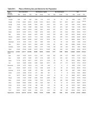
IntroductionThe results <strong>of</strong> the poverty analysis are mapped toprovide <strong>in</strong>formation for policy makers <strong>and</strong> others, thatis relatively easy to underst<strong>and</strong> <strong>and</strong> use. Work<strong>in</strong>g withpoverty maps based on census data that coversevery household <strong>in</strong> the country, as opposed towork<strong>in</strong>g with only a small sample <strong>of</strong> the population,improves our underst<strong>and</strong><strong>in</strong>g <strong>of</strong> the evolution <strong>and</strong>distribution <strong>of</strong> poverty <strong>in</strong> three important ways.First, it allows us to study poverty at a highlydisaggregated level—<strong>in</strong> the case <strong>of</strong> Ug<strong>and</strong>a, at thelevel <strong>of</strong> the sub-county for rural areas <strong>and</strong> parishfor urban areas. Second, it makes it possible toderive st<strong>and</strong>ard errors for our poverty figures thatlet us know the level <strong>of</strong> accuracy with which weare measur<strong>in</strong>g poverty <strong>and</strong> changes <strong>in</strong> poverty.Third, hav<strong>in</strong>g detailed maps <strong>of</strong> both rates <strong>and</strong>concentration <strong>of</strong> poverty enables policy makers<strong>and</strong> the public to set policy goals <strong>in</strong> a transparentmanner <strong>and</strong> to track results over time.The percentage change <strong>in</strong> rural poverty <strong>in</strong>cidenceat sub-county level between 1992 <strong>and</strong> 2002 ispresented <strong>in</strong> Map 1.1. The level <strong>of</strong> change <strong>in</strong>poverty <strong>in</strong> each sub-county is mapped us<strong>in</strong>g acategorical six-colour scheme. This is divided <strong>in</strong>to twomajor categories. First is the group that has witnessedreductions <strong>in</strong> poverty <strong>in</strong>cidence. For this category, thecolours range from dark green, <strong>in</strong>dicat<strong>in</strong>g sub-countiesthat have experienced huge reductions <strong>in</strong> poverty,to light green for sub-counties that have witnessedrelatively lower reductions <strong>in</strong> poverty. Second is thecategory that has experienced <strong>in</strong>crements <strong>in</strong> poverty.In this category, the colours range from dark brownfor areas that have experienced large <strong>in</strong>crements <strong>in</strong>poverty, to light brown for those sub-counties whose<strong>in</strong>crements <strong>in</strong> poverty level are relatively lower.The results <strong>of</strong> the analysis <strong>of</strong> changes <strong>in</strong> poverty levelsfrom 1992–2002 are encourag<strong>in</strong>g, show<strong>in</strong>g widespread<strong>and</strong> large decreases <strong>in</strong> the <strong>in</strong>cidence <strong>of</strong> povertyacross Ug<strong>and</strong>a. Ga<strong>in</strong>s <strong>in</strong> poverty reduction are welldistributed <strong>in</strong> almost all the regions, except for a fewpockets <strong>in</strong> the Karamoja sub region (Map 1.1). Thehighest drops <strong>in</strong> rural poverty <strong>in</strong>cidence are seen <strong>in</strong>sub-counties across Western <strong>and</strong> Central regions.<strong>Poverty</strong> was estimated to have <strong>in</strong>creased <strong>in</strong> a few subcounties<strong>in</strong> Northern Region.6 <strong>Nature</strong>, distribution <strong>and</strong> evolution <strong>of</strong> poverty <strong>and</strong> <strong>in</strong>equality <strong>in</strong> Ug<strong>and</strong>a, 1992 - 2002
IntroductionMap 1.1Percentage change <strong>in</strong> rural poverty <strong>in</strong>cidence by sub-county from1992 to 2002<strong>Nature</strong>, distribution <strong>and</strong> evolution <strong>of</strong> poverty <strong>and</strong> <strong>in</strong>equality <strong>in</strong> Ug<strong>and</strong>a, 1992 - 2002 7
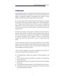
Concepts, methods <strong>and</strong> data2.3 <strong>Poverty</strong> density measureThe poverty <strong>in</strong>cidence measure does not provide<strong>in</strong>formation as to the number <strong>of</strong> poor people <strong>in</strong>a given area. For example, some sub-counties onthis map have high poverty rates, but are <strong>in</strong>habitedby relatively few people. As <strong>in</strong> other countries,decision makers <strong>in</strong> Ug<strong>and</strong>a are <strong>of</strong>ten <strong>in</strong>terested <strong>in</strong>the distribution <strong>of</strong> the poor, i.e. where the highestnumbers <strong>of</strong> poor are found among adm<strong>in</strong>istrativeunits <strong>and</strong> constituencies. The poverty densitymeasure provides this <strong>in</strong>formation.The poverty density measures the number <strong>of</strong> poorpeople per square kilometre <strong>in</strong> a sub-county orgiven area. The poverty density <strong>of</strong> each sub-countyis mapped us<strong>in</strong>g a categorical seven-colour schemethat ranges from light peach <strong>in</strong>dicat<strong>in</strong>g relativelylow density to dark brown for high density areas.The poverty density <strong>of</strong> each <strong>of</strong> the sub-counties<strong>in</strong> Northern Region is shown <strong>in</strong> Map 2.2. Dadamusub-county <strong>in</strong> Ayivu County, Arua District, hasthe highest poverty density <strong>in</strong> the region yet it isnot the poorest sub-county accord<strong>in</strong>g to poverty<strong>in</strong>cidence (Map 2.1). Exam<strong>in</strong><strong>in</strong>g the povertydensity maps, which present the number <strong>of</strong> poorpeople per km 2 , alongside the poverty <strong>in</strong>cidencemaps, provides valuable <strong>and</strong> complementary<strong>in</strong>formation regard<strong>in</strong>g the geographic dimensions<strong>of</strong> poverty <strong>in</strong> Ug<strong>and</strong>a.14 <strong>Nature</strong>, distribution <strong>and</strong> evolution <strong>of</strong> poverty <strong>and</strong> <strong>in</strong>equality <strong>in</strong> Ug<strong>and</strong>a, 1992 - 200214
Concepts, methods <strong>and</strong> dataMap 2.2 Interpret<strong>in</strong>g the <strong>Poverty</strong> Density Measure:Northern Region sub-county-level <strong>Poverty</strong> Density<strong>Nature</strong>, distribution <strong>and</strong> evolution <strong>of</strong> poverty <strong>and</strong> <strong>in</strong>equality <strong>in</strong> Ug<strong>and</strong>a, 1992 - 2002 15
Concepts, methods <strong>and</strong> data2.4 <strong>Poverty</strong> gap measureThe poverty <strong>in</strong>cidence measure does not <strong>in</strong>dicatehow poor the poor are. It does not dist<strong>in</strong>guishbetween a household whose consumption levelsare very close to the poverty l<strong>in</strong>e <strong>and</strong> a householdwhose consumption levels are far below it. Ifpeople below the poverty l<strong>in</strong>e were to becomepoorer, this measure does not change. The povertygap measure overcomes this problem.The poverty gap provides <strong>in</strong>formation onthe depth <strong>of</strong> poverty. It captures the averageexpenditure shortfall, or gap, for the poor <strong>in</strong> agiven area to reach the poverty l<strong>in</strong>e. The povertygap is obta<strong>in</strong>ed by add<strong>in</strong>g up all the shortfalls <strong>of</strong>the poor (ignor<strong>in</strong>g the non-poor) <strong>and</strong> divid<strong>in</strong>gthis total by the number <strong>of</strong> poor. It measures thepoverty deficit <strong>of</strong> the population or the resourcesthat would be needed to lift all the poor <strong>in</strong> thatarea out <strong>of</strong> poverty, if one were able to perfectlytarget cash transfers towards clos<strong>in</strong>g the gap. Inthis sense, the poverty gap is a very crude measure<strong>of</strong> the m<strong>in</strong>imum amount <strong>of</strong> resources necessary toeradicate poverty, i.e. the amount <strong>of</strong> money thatwould have to be transferred to the poor to liftthem up to the poverty l<strong>in</strong>e, under an assumption<strong>of</strong> perfect target<strong>in</strong>g.To demonstrate, aga<strong>in</strong> us<strong>in</strong>g Northern Region asan example, results <strong>of</strong> this analysis suggest that<strong>in</strong> 2002 the poverty gap for the rural population<strong>in</strong> Northern Region was 24.3% (UBOS 2003). Thisimplies that, on average, every poor person <strong>in</strong> arural area <strong>in</strong> the Northern Region would requirean additional UShs 5,071 per month to reach thepoverty l<strong>in</strong>e (i.e. 24.3% <strong>of</strong> the UShs 20,872 ruralpoverty l<strong>in</strong>e). Thus, if 65% <strong>of</strong> the rural populationwas poor (accord<strong>in</strong>g to the headcount <strong>in</strong>dex) <strong>in</strong>2002, imply<strong>in</strong>g roughly 3.1 million poor people<strong>in</strong> Northern Region, approximately UShs 15.8billion (US$ 8.7 million) per month would havebeen needed, <strong>in</strong> perfectly targeted cash transfers,to eradicate rural poverty <strong>in</strong> Northern Ug<strong>and</strong>a <strong>in</strong>2002.The poverty gap for Northern Region at the subcountylevel is shown <strong>in</strong> Map 2.3. The green areasshow relatively low poverty gaps <strong>and</strong> the greyshad<strong>in</strong>g <strong>in</strong>dicates high poverty gaps. The highestpoverty gap is found <strong>in</strong> Lopei (55%) <strong>in</strong> MorotoDistrict. This implies that, on average, every poorperson <strong>in</strong> this region would require an additionalUShs 11,508 per month to reach the poverty l<strong>in</strong>e.Therefore, to pull all the poor people (30,558)<strong>in</strong> this sub-county (with an overall population<strong>of</strong> 31,182 people <strong>and</strong> poverty rate <strong>of</strong> 98%) to thepoverty l<strong>in</strong>e would require UShs 352 million (US$193,646; 1US$ = UShs. 1816) per month. Decisionmakers could use this <strong>in</strong>formation to identify areas<strong>of</strong> deep (or shallow) poverty <strong>and</strong> to estimate howmuch it would cost to raise st<strong>and</strong>ards <strong>of</strong> liv<strong>in</strong>g <strong>in</strong>such areas.However, like the head count <strong>in</strong>dex or poverty<strong>in</strong>cidence, the poverty gap measure has someshortcom<strong>in</strong>gs. First, it is neither practical norfeasible to reach the whole population throughperfectly targeted cash transfers. Second, it doesnot measure <strong>in</strong>equality among poor people, i.e.the fact that some people might only be a fewshill<strong>in</strong>gs short <strong>of</strong> the poverty l<strong>in</strong>e while othersmight only have a few shill<strong>in</strong>gs to spend. The G<strong>in</strong>icoefficient is a measure that captures this range<strong>in</strong> people’s expenditures/<strong>in</strong>comes, i.e. it is a proxyfor <strong>in</strong>come <strong>in</strong>equality.16 <strong>Nature</strong>, distribution <strong>and</strong> evolution <strong>of</strong> poverty <strong>and</strong> <strong>in</strong>equality <strong>in</strong> Ug<strong>and</strong>a, 1992 - 2002
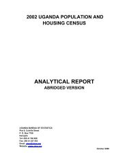
Concepts, methods <strong>and</strong> data2.5 The <strong>in</strong>equality measure, G<strong>in</strong>i coefficientThe previous sections discuss the poverty measures<strong>and</strong> focus on where <strong>in</strong>dividuals f<strong>in</strong>d themselves<strong>in</strong> relation to the poverty l<strong>in</strong>e. They thereforeprovide statistics summariz<strong>in</strong>g the bottom <strong>of</strong> theconsumption distribution (i.e. those that fall belowthe poverty l<strong>in</strong>e). In this report <strong>in</strong>equality refers tothe dispersion <strong>of</strong> the distribution over the entire(estimated) consumption aggregate. There are anumber <strong>of</strong> <strong>in</strong>dices used to measure <strong>in</strong>equality <strong>and</strong>these <strong>in</strong>clude the Theil Entropy <strong>in</strong>dex, coefficient<strong>of</strong> variation <strong>and</strong> the G<strong>in</strong>i coefficient. The mostwidely used measure <strong>of</strong> <strong>in</strong>equality is the G<strong>in</strong>i <strong>in</strong>dex.It ranges from zero (<strong>in</strong>dicat<strong>in</strong>g perfect equality,i.e. where everyone <strong>in</strong> the population has thesame expenditure or <strong>in</strong>come) to one (<strong>in</strong>dicat<strong>in</strong>gperfect <strong>in</strong>equality, i.e. when all expenditure or<strong>in</strong>come is accounted for by a s<strong>in</strong>gle person <strong>in</strong> thepopulation). A high value <strong>of</strong> the G<strong>in</strong>i coefficientimplies that a few people have most <strong>of</strong> the <strong>in</strong>comeor consumption <strong>and</strong> the majority has less. Formost develop<strong>in</strong>g countries, the G<strong>in</strong>i <strong>in</strong>dex rangesbetween 0.3 <strong>and</strong> 0.6 (World Bank, 2005).Once aga<strong>in</strong>, we demonstrate how to <strong>in</strong>terpretthe <strong>in</strong>equality maps us<strong>in</strong>g Northern Ug<strong>and</strong>a asan example. The G<strong>in</strong>i coefficient for sub-counties<strong>in</strong> Northern Ug<strong>and</strong>a is shown <strong>in</strong> Map 2.4. Thep<strong>in</strong>k areas show relatively high <strong>in</strong>equality with<strong>in</strong>sub-counties <strong>and</strong> the light green shad<strong>in</strong>g showsareas with low <strong>in</strong>equality. The map <strong>in</strong>dicates that<strong>in</strong>equality is heterogeneously distributed <strong>in</strong> theregion. There are no sub-counties with <strong>in</strong>equalitylevels below 0.25 <strong>and</strong> there are 38 sub-countieswith G<strong>in</strong>i coefficients above 0.40. For <strong>in</strong>stance,the least poor sub-county <strong>of</strong> Namasale <strong>in</strong> KiogaCounty also has the one <strong>of</strong> the highest <strong>in</strong>equalitylevels (0.47) <strong>in</strong> the region. This implies that a largeproportion <strong>of</strong> the <strong>in</strong>come or consumption <strong>in</strong> thesub-county is owned by a few households. Incontrast, the lowest <strong>in</strong>equality (less than 0.25) <strong>in</strong>the region is found <strong>in</strong> Lopei Sub-county (imply<strong>in</strong>gthat the <strong>in</strong>come or consumption is generallyowned by many households). This sub-county hasan 89% poverty rate, imply<strong>in</strong>g virtually everyoneis poor. We discuss these distributions <strong>in</strong> moredetail <strong>in</strong> the next chapter.18 <strong>Nature</strong>, distribution <strong>and</strong> evolution <strong>of</strong> poverty <strong>and</strong> <strong>in</strong>equality <strong>in</strong> Ug<strong>and</strong>a, 1992 - 2002
Concepts, methods <strong>and</strong> dataMap 2.4 Interpret<strong>in</strong>g the Income <strong>Inequality</strong> Measure:Northern Region sub-county-level G<strong>in</strong>i Coefficient Example<strong>Nature</strong>, distribution <strong>and</strong> evolution <strong>of</strong> poverty <strong>and</strong> <strong>in</strong>equality <strong>in</strong> Ug<strong>and</strong>a, 1992 - 2002 19
Concepts, methods <strong>and</strong> data2.6 <strong>Poverty</strong> mapp<strong>in</strong>g methodology <strong>and</strong> the dataThe methodology used to map poverty (described<strong>in</strong> detail <strong>in</strong> Appendix 1) <strong>in</strong>volves detailed analysis<strong>of</strong> two ma<strong>in</strong> sources <strong>of</strong> data: the population<strong>and</strong> hous<strong>in</strong>g census <strong>and</strong> a household welfaremonitor<strong>in</strong>g survey. In certa<strong>in</strong> cases, additionaldata can be obta<strong>in</strong>ed from environmental statistics<strong>and</strong> sector-specific surveys. In the first step <strong>of</strong> theanalysis, the two data sources are subjected to veryclose scrut<strong>in</strong>y with emphasis on identify<strong>in</strong>g a set<strong>of</strong> common variables. These variables will formthe set from which we will choose key variablesfor our <strong>in</strong>come <strong>and</strong> consumption models <strong>in</strong> thesecond step. More precisely, <strong>in</strong> this stage thesurvey is used to develop a series <strong>of</strong> statisticalmodels which relate per capita consumption tothe set <strong>of</strong> common variables identified <strong>in</strong> thepreced<strong>in</strong>g step. After this, <strong>in</strong> the third <strong>and</strong> f<strong>in</strong>alstep <strong>of</strong> the analysis, the parameter estimates fromthe previous stage are applied to the populationcensus <strong>and</strong> used to predict consumption for eachhousehold <strong>in</strong>cluded <strong>in</strong> the census. Once such apredicted consumption measure is available foreach household <strong>in</strong> the census, summary measures<strong>of</strong> poverty <strong>and</strong> <strong>in</strong>equality can be estimated foran aggregated set <strong>of</strong> households <strong>in</strong> the census.Statistical tests can be performed to assess thereliability <strong>of</strong> the aggregated poverty estimates thathave been produced.These three stages <strong>of</strong> analysis occur <strong>in</strong> sequence.In the first stage <strong>of</strong> the poverty mapp<strong>in</strong>g exercise,we consider household asset, demographic<strong>and</strong> occupational variables that are plausiblycorrelated with <strong>in</strong>come or consumption. Thisis a rather pa<strong>in</strong>stak<strong>in</strong>g comparison <strong>of</strong> commonvariables found <strong>in</strong> both the household survey <strong>and</strong>the population census. The idea here is to identifyvariables at the household level that are def<strong>in</strong>ed<strong>in</strong> the same way <strong>in</strong> both the household survey <strong>and</strong>the census. It is important that this common subset<strong>of</strong> variables be def<strong>in</strong>ed <strong>in</strong> exactly the same wayacross the two data sources; this is verified us<strong>in</strong>gstatistical tests <strong>of</strong> differences <strong>of</strong> the means.Concurrently, with the exercise described above, adatabase is compiled at a level <strong>of</strong> aggregation higherthan the household <strong>and</strong> jo<strong>in</strong>ed with the householdlevel census <strong>and</strong> the household survey databases(Lanjouw 2004). This data conta<strong>in</strong>s geographic<strong>in</strong>formation on l<strong>and</strong> use, for example. A keymethodological concern <strong>in</strong> the poverty mapp<strong>in</strong>gexercise is that the common pool <strong>of</strong> householdvariables cannot capture unobserved geographiceffects, such as l<strong>and</strong> use <strong>and</strong> agro-climaticconditions, which might still be very important<strong>in</strong> predict<strong>in</strong>g household level consumption. For<strong>in</strong>stance, Okwi et al. (2005, 2006) <strong>in</strong>corporatedl<strong>and</strong> use <strong>and</strong> environmental data for Ug<strong>and</strong>a <strong>in</strong>their models to estimate the l<strong>in</strong>k between theenvironment <strong>and</strong> poverty. These supplementalsub--district level data conta<strong>in</strong> a wide range <strong>of</strong>variables <strong>in</strong>clud<strong>in</strong>g roads <strong>and</strong> road buffers, distanceto water, proportions <strong>of</strong> l<strong>and</strong> under different l<strong>and</strong>use types, protected areas such as forest <strong>and</strong> gameparks, population estimates etc. 5The comprehensive database is then used t<strong>of</strong>ormulate a model that estimates householdconsumption <strong>in</strong> the household survey as afunction <strong>of</strong> the <strong>in</strong>dependent variables that passthe first step. This can only be achieved if thetwo tasks described above yield a good <strong>and</strong>reasonably large set <strong>of</strong> common household-levelvariables, supplemented by a series <strong>of</strong> additional(geographic/community-level) variables at a slightlyhigher level <strong>of</strong> disaggregation (enumerationarea (EA) or sub-district level). Inclusion <strong>of</strong> thesecommunity-level variables is meant to improvethe explanatory power <strong>of</strong> the model (Lanjouw,2004). We pick the household variables that bestcorrelate with household level variation <strong>in</strong> percapita consumption. Basically, this stage <strong>in</strong>volvesthe econometric estimation <strong>of</strong> different models foreach stratum <strong>in</strong> the household survey data set, runseparately for rural <strong>and</strong> urban areas.5See Okwi et al. (2006) for a detailed discussion <strong>of</strong> this approach.20 <strong>Nature</strong>, distribution <strong>and</strong> evolution <strong>of</strong> poverty <strong>and</strong> <strong>in</strong>equality <strong>in</strong> Ug<strong>and</strong>a, 1992 - 2002
Concepts, methods <strong>and</strong> dataIn the third step <strong>of</strong> the analysis, we obta<strong>in</strong> theparameter estimates <strong>and</strong> attendant statisticaloutputs from the second step <strong>and</strong> generateestimates <strong>and</strong> confidence <strong>in</strong>tervals for the poverty<strong>and</strong> <strong>in</strong>equality <strong>in</strong>dices. In other words, this step isassociated with the imputation <strong>of</strong> consumption<strong>in</strong>to the census data at the household level <strong>and</strong>the estimation <strong>of</strong> poverty <strong>and</strong> <strong>in</strong>equality measuresat the appropriate levels <strong>of</strong> spatial disaggregation.However, the appropriate level <strong>of</strong> spatialdisaggregation depends upon the magnitude <strong>of</strong>the st<strong>and</strong>ard errors.The f<strong>in</strong>al step <strong>in</strong>volves mapp<strong>in</strong>g the poverty <strong>and</strong><strong>in</strong>equality figures. We use the databases thatprovide the estimates <strong>of</strong> poverty <strong>and</strong> <strong>in</strong>equality(<strong>and</strong> their st<strong>and</strong>ard errors) at a variety <strong>of</strong> levels<strong>of</strong> geographic disaggregation. These figures areprojected onto geographic maps at differentadm<strong>in</strong>istrative or even socio-economic levelsus<strong>in</strong>g Geographic Information System (GIS)mapp<strong>in</strong>g techniques. This <strong>in</strong>volves the application<strong>of</strong> GIS s<strong>of</strong>tware (such as Arcview) which merges<strong>in</strong>formation on the geographic coord<strong>in</strong>ates <strong>of</strong>localities such as the district or sub-county withthe poverty <strong>and</strong> <strong>in</strong>equality estimates producedby the poverty mapp<strong>in</strong>g methodology. Additionaldetails on the poverty mapp<strong>in</strong>g analysis <strong>and</strong> morereferences are provided <strong>in</strong> Appendix 1.Ensur<strong>in</strong>g comparability across the maps for 1992<strong>and</strong> 2002, however, was relatively easy given thatthe expenditure modules used <strong>in</strong> the 1992 <strong>and</strong>2002 household surveys were identical, so thatwe did not need to construct new comparableconsumption aggregates <strong>in</strong> order to producecomparable poverty figures. F<strong>in</strong>ally, it is importantto mention that we were unable to produce povertyfigures for Kotido District, s<strong>in</strong>ce the data showedmajor <strong>in</strong>consistencies. This is an important caveat<strong>in</strong> our analysis <strong>and</strong> it should teach us a lesson – noeconometric method or approximation is a goodenough substitute for primary data.<strong>Nature</strong>, distribution <strong>and</strong> evolution <strong>of</strong> poverty <strong>and</strong> <strong>in</strong>equality <strong>in</strong> Ug<strong>and</strong>a, 1992 - 200221
22 <strong>Nature</strong>, distribution <strong>and</strong> evolution <strong>of</strong> poverty <strong>and</strong> <strong>in</strong>equality <strong>in</strong> Ug<strong>and</strong>a, 1992 - 2002
Chapter 3<strong>Distribution</strong> <strong>and</strong> evolution <strong>of</strong> poverty<strong>and</strong> <strong>in</strong>equality <strong>in</strong> 1992 - 2002In this chapter we provide an overview <strong>of</strong> the state <strong>and</strong> changes <strong>in</strong> poverty <strong>and</strong> <strong>in</strong>equality conditions <strong>in</strong>Ug<strong>and</strong>a between 1992 <strong>and</strong> 2002 (the year for which the most recent data are available at national level).We present poverty <strong>and</strong> <strong>in</strong>equality measures for 2002 <strong>and</strong> exam<strong>in</strong>e how these figures have changeds<strong>in</strong>ce 1992. In Ug<strong>and</strong>a, because the adm<strong>in</strong>istrative boundaries have changed significantly from 39 districts<strong>in</strong> 1992 to 56 districts <strong>in</strong> 2002, we cannot precisely analyse the changes <strong>in</strong> poverty at district level. However,we can analyse the changes at the county <strong>and</strong> sub-county levels, s<strong>in</strong>ce these adm<strong>in</strong>istrative units have notchanged significantly. This chapter presents a summary <strong>of</strong> the estimates for each region <strong>and</strong> the completeset <strong>of</strong> poverty <strong>and</strong> <strong>in</strong>equality measures for each county <strong>and</strong> sub-county are presented <strong>in</strong> Tables A3 <strong>and</strong> A4<strong>in</strong> Appendix 2.3.1 <strong>Poverty</strong> <strong>and</strong> <strong>in</strong>equality <strong>in</strong> Ug<strong>and</strong>a <strong>in</strong> 2002We construct poverty <strong>and</strong> <strong>in</strong>equality measuresfor 2002 us<strong>in</strong>g the 2002/03 Ug<strong>and</strong>a NationalHousehold Survey (UNHS II) <strong>and</strong> the 2002Population <strong>and</strong> Hous<strong>in</strong>g Census follow<strong>in</strong>g themethodology described <strong>in</strong> the previous chapter.We use consumption-based measures s<strong>in</strong>ceconsumption fluctuates less than <strong>in</strong>come dur<strong>in</strong>gthe course <strong>of</strong> a particular year or month, <strong>and</strong>people tend to report on their consumption <strong>and</strong>expenditures more accurately than they report<strong>in</strong>come.In this analysis, poverty measures are constructedas a function <strong>of</strong> the poverty l<strong>in</strong>e, among otherth<strong>in</strong>gs. The poverty l<strong>in</strong>e for 2002 is set to 1997prices so that it is comparable to that <strong>of</strong> 1992. 6This allows us to produce comparable povertyestimates for the decade 1992–2002. The values<strong>of</strong> the poverty l<strong>in</strong>es presented here are adoptedfrom the <strong>of</strong>ficial monthly per capita poverty l<strong>in</strong>esused by UBOS (also summary <strong>in</strong> Table 2.1) <strong>and</strong>are strictly comparable with the ones presented<strong>in</strong> earlier reports by the same <strong>in</strong>stitution. <strong>Poverty</strong>l<strong>in</strong>es for 1992 are presented <strong>in</strong> the earlier series<strong>of</strong> this report (see UBOS <strong>and</strong> ILRI 2004).The previous poverty <strong>and</strong> <strong>in</strong>equality estimatesbased on surveys were designed to berepresentative at the regional level. Both ouranalyses us<strong>in</strong>g the 1992 household survey<strong>and</strong> 1991 census <strong>and</strong> the 2002 data are able toproduce poverty estimates at the regional level<strong>and</strong> lower adm<strong>in</strong>istrative levels. In 1992, theestimates were at the county level for rural areaswhile for the urban areas the estimates were atsub-county level. This current analysis goes astep lower <strong>and</strong> produces poverty <strong>and</strong> <strong>in</strong>equalityestimates at all levels from the region to the subcounty.The 2002 poverty <strong>and</strong> <strong>in</strong>equality estimatesare entirely consistent with the earlier surveyestimates because <strong>of</strong> the similarities <strong>in</strong> the survey<strong>and</strong> census questionnaires <strong>in</strong> both years <strong>and</strong> thedemonstrated robustness <strong>of</strong> the method.At national level, our analysis leads to anestimated national poverty head count <strong>of</strong> 38.8%<strong>in</strong> 2002. The poor, however, were not uniformlydistributed across areas <strong>and</strong> regions. <strong>Poverty</strong>was more prevalent <strong>in</strong> rural areas. <strong>Poverty</strong> wasalso deeper <strong>in</strong> the rural areas than it was <strong>in</strong> theurban areas (as measured by the poverty gap).In contrast, the level <strong>of</strong> <strong>in</strong>equality <strong>of</strong> <strong>in</strong>come(represented by consumption expenditure) washigher <strong>in</strong> urban than <strong>in</strong> rural areas. These broadpatterns are consistent with those reported <strong>in</strong>previous poverty reports (see UBOS 2003).6Both the poverty l<strong>in</strong>es for 1992 <strong>and</strong> 2002 have been adjusted to 1997 prices (see UBOS 2003).<strong>Nature</strong>, distribution <strong>and</strong> evolution <strong>of</strong> poverty <strong>and</strong> <strong>in</strong>equality <strong>in</strong> Ug<strong>and</strong>a, 1992 - 2002 23
<strong>Distribution</strong> <strong>and</strong> evolution <strong>of</strong> poverty <strong>and</strong> <strong>in</strong>equality <strong>in</strong> 1992 - 20023.2 <strong>Poverty</strong> <strong>in</strong> rural <strong>and</strong> urban areas, 2002There are marked differences <strong>in</strong> poverty <strong>and</strong><strong>in</strong>equality across Ug<strong>and</strong>a’s four regions. In ruralareas, the predictions based on the census showthat poverty <strong>in</strong>cidence was highest <strong>in</strong> the NorthernRegion, <strong>and</strong> lowest <strong>in</strong> Central Region (with 66%<strong>and</strong> 27% <strong>of</strong> the population liv<strong>in</strong>g below thepoverty l<strong>in</strong>e respectively). These predictions showthat the rank<strong>in</strong>gs <strong>of</strong> the rural areas <strong>in</strong> the Western<strong>and</strong> Eastern regions (34% <strong>and</strong> 47% respectively),are consistent with the survey estimates obta<strong>in</strong>edby UBOS (2003). Only the Northern Region 7 hada rural poverty rate higher than 50%. In terms <strong>of</strong>the other poverty measures, similar patterns canbe seen. The poverty gap estimates were highestfor Northern Region (27%) <strong>and</strong> lowest <strong>in</strong> CentralRegion (7 percent). However, the poverty densitymeasure shows that the highest poverty densitiesare found <strong>in</strong> Eastern Region, with much <strong>of</strong> theregion hav<strong>in</strong>g more than 175 poor people persquare kilometre. This clearly shows that highpoverty rates do not necessarily reflect high povertydensities because <strong>of</strong> the spatial distribution <strong>of</strong> thepoor. F<strong>in</strong>ally, the highest <strong>in</strong>equality <strong>of</strong> <strong>in</strong>comes isfound <strong>in</strong> the Eastern Region (0.42) imply<strong>in</strong>g thebiggest proportion <strong>of</strong> the wealth is owned by afew people, <strong>and</strong> the lowest is <strong>in</strong> Western Region(0.35).In urban areas, Northern Region still has the highestpoverty rates. When Kampala is excluded from theCentral Region, the lowest poverty rate as expectedis found <strong>in</strong> Kampala (5 percent). Interest<strong>in</strong>gly, theEastern Region has the lowest urban poverty rate(15.9%) compared with Central without Kampala.The poverty gap shows a consistent picture. TheNorth has the highest poverty gap (13%) whileKampala has the lowest poverty gap (1.10 percent).When the G<strong>in</strong>i coefficient was considered, theCentral Region (with or without Kampala) had thehighest <strong>in</strong>equality figures. The lowest <strong>in</strong>equality isaga<strong>in</strong> observed <strong>in</strong> Western Region.District, county <strong>and</strong> sub-county level estimatesbased on the adm<strong>in</strong>istrative boundaries used <strong>in</strong>2002 are presented. Disaggregation to the lowestlevel <strong>of</strong> adm<strong>in</strong>istration, the sub-county, adds asignificant amount <strong>of</strong> detail to the poverty analysiscompared to the previous analysis which stoppedat the county level. Detailed statistics fromthe census-based po<strong>in</strong>t estimates for all theseadm<strong>in</strong>istrative units for rural <strong>and</strong> urban areas(respectively) are presented <strong>in</strong> Tables A3 <strong>and</strong> A4. 87Kotido District <strong>in</strong> Northern Ug<strong>and</strong>a is excluded due to data limitations.8The st<strong>and</strong>ard errors <strong>in</strong> this analysis were consistently lower than the survey-based estimates (see UBOS 2003) <strong>in</strong>dicat<strong>in</strong>gthe census-based estimates are more precise (due to additional <strong>in</strong>formation ga<strong>in</strong>ed by l<strong>in</strong>k<strong>in</strong>g the two data sets<strong>and</strong> the robustness <strong>of</strong> the methodology). See Appendix 1 for details.24 <strong>Nature</strong>, distribution <strong>and</strong> evolution <strong>of</strong> poverty <strong>and</strong> <strong>in</strong>equality <strong>in</strong> Ug<strong>and</strong>a, 1992 - 2002
<strong>Distribution</strong> <strong>and</strong> evolution <strong>of</strong> poverty <strong>and</strong> <strong>in</strong>equality <strong>in</strong> 1992 - 2002Map 3.1Ug<strong>and</strong>a 2002 - Region-Level <strong>Poverty</strong> Incidence<strong>Nature</strong>, distribution <strong>and</strong> evolution <strong>of</strong> poverty <strong>and</strong> <strong>in</strong>equality <strong>in</strong> Ug<strong>and</strong>a, 1992 - 2002 25
<strong>Distribution</strong> <strong>and</strong> evolution <strong>of</strong> poverty <strong>and</strong> <strong>in</strong>equality <strong>in</strong> 1992 - 20023.3 Summary <strong>of</strong> poverty estimates by region, 2002Central regionThe Central Region is still generally the least poorregion <strong>in</strong> Ug<strong>and</strong>a. In rural areas, at the districtlevel, the poverty rates ranged from 8 percent to36%. Accord<strong>in</strong>g to this census-based analysis, theleast poor sub-county was Maz<strong>in</strong>ga <strong>in</strong> KyamuswaCounty <strong>of</strong> Kalangala District with only 2 percent<strong>of</strong> the people liv<strong>in</strong>g below the poverty l<strong>in</strong>e. Incontrast, Gayaza sub-county <strong>in</strong> Kiboga County,Kiboga District, was the poorest sub-county with apoverty <strong>in</strong>cidence <strong>of</strong> 47%.At the county level, the poorest county was Bbaale<strong>in</strong> Kayunga District, which was also the poorestdistrict. Kampala st<strong>and</strong>s out as the least poor districtamong urban areas with a poverty <strong>in</strong>cidence <strong>of</strong>only 6 percent. The poorest urban-based districtwas Nakasongola (27%). Kooki County <strong>in</strong> RakaiDistrict was the poorest urban county (28%) <strong>and</strong>Nkokonjeru <strong>in</strong> Buikwe County, Mukono District,was the poorest urban sub-county <strong>in</strong> this region.Mak<strong>in</strong>dye Division 9 (5 percent) had the lowestpoverty rates among all the urban sub-counties.The rural poverty gap was highest <strong>in</strong> Gayaza Subcounty<strong>in</strong> Kiboga County, Kiboga District (14.2)<strong>and</strong> lowest <strong>in</strong> Maz<strong>in</strong>ga <strong>in</strong> Kyamuswa County <strong>of</strong>Kalangala District. For the urban areas Kampalahad the lowest poverty gap. The low poverty gap <strong>in</strong>Kampala suggests that the poor are relatively closeto the poverty l<strong>in</strong>e, so the resources required tomove people out <strong>of</strong> poverty are not as high as forthose with large poverty gaps.In terms <strong>of</strong> number <strong>of</strong> poor, Kayunga District hasthe highest poverty density, at 66 poor personsper km 2 , while Kalangala District has only 5 poorpeople per km2. Mov<strong>in</strong>g down to the sub-countylevel, Nabweru Sub-county <strong>in</strong> Kyadondo County,Wakiso District, had the highest poverty density<strong>of</strong> 201 poor per km 2 compared with Ngoma <strong>in</strong>Nakaseke County, Luwero District (2 poor perkm 2 ). Among the urban areas, Kampala had thehighest poverty density (312 poor per km 2 ).Our <strong>in</strong>equality measure shows a range <strong>of</strong> 0.28 to0.40 across sub-counties <strong>in</strong> Central Region. For ruralsub-counties, the highest <strong>in</strong>equality was found <strong>in</strong>Kiira (Kyadondo County, Wakiso District) <strong>and</strong> thelowest <strong>in</strong> Butoloogo (Buwekula County, MubendeDistrict). For urban areas, exclud<strong>in</strong>g Kampala, 10 thehighest <strong>in</strong>equality <strong>in</strong> Central Region was <strong>in</strong> DivisionA (0.62) (Entebbe Municipality, Wakiso District)<strong>and</strong> lowest <strong>in</strong> Rakai Town Council (0.37) (KookiCounty, Rakai District). A high variability is seen <strong>in</strong><strong>in</strong>equality <strong>in</strong>dices at all levels. Maps 3.2 to 3.6 showthe different poverty <strong>and</strong> <strong>in</strong>equality measures forCentral Region.9In urban areas, a division is the equivalent <strong>of</strong> a sub-county <strong>in</strong> rural areas.10Kampala is treated as a separate region because <strong>of</strong> its unique features as a capital city.26 <strong>Nature</strong>, distribution <strong>and</strong> evolution <strong>of</strong> poverty <strong>and</strong> <strong>in</strong>equality <strong>in</strong> Ug<strong>and</strong>a, 1992 - 2002
<strong>Distribution</strong> <strong>and</strong> evolution <strong>of</strong> poverty <strong>and</strong> <strong>in</strong>equality <strong>in</strong> 1992 - 2002Map 3.2 Central Region, 2002 – Sub-county level <strong>Poverty</strong> Incidence<strong>Nature</strong>, distribution <strong>and</strong> evolution <strong>of</strong> poverty <strong>and</strong> <strong>in</strong>equality <strong>in</strong> Ug<strong>and</strong>a, 1992 - 2002 27
<strong>Distribution</strong> <strong>and</strong> evolution <strong>of</strong> poverty <strong>and</strong> <strong>in</strong>equality <strong>in</strong> 1992 - 2002Map 3.3Central Region, 2002 – Sub-county level <strong>Poverty</strong> Gap28 <strong>Nature</strong>, distribution <strong>and</strong> evolution <strong>of</strong> poverty <strong>and</strong> <strong>in</strong>equality <strong>in</strong> Ug<strong>and</strong>a, 1992 - 2002
<strong>Distribution</strong> <strong>and</strong> evolution <strong>of</strong> poverty <strong>and</strong> <strong>in</strong>equality <strong>in</strong> 1992 - 2002Map 3.4 Central Region, 2002 – Sub-county level G<strong>in</strong>i coefficient<strong>Nature</strong>, distribution <strong>and</strong> evolution <strong>of</strong> poverty <strong>and</strong> <strong>in</strong>equality <strong>in</strong> Ug<strong>and</strong>a, 1992 - 2002 29
<strong>Distribution</strong> <strong>and</strong> evolution <strong>of</strong> poverty <strong>and</strong> <strong>in</strong>equality <strong>in</strong> 1992 - 2002Map 3.5Kampala, 2002 – Parish-level <strong>Poverty</strong> Incidence30 <strong>Nature</strong>, distribution <strong>and</strong> evolution <strong>of</strong> poverty <strong>and</strong> <strong>in</strong>equality <strong>in</strong> Ug<strong>and</strong>a, 1992 - 2002
<strong>Distribution</strong> <strong>and</strong> evolution <strong>of</strong> poverty <strong>and</strong> <strong>in</strong>equality <strong>in</strong> 1992 - 2002Map 3.6Masaka, 2002 – <strong>Poverty</strong> Incidence<strong>Nature</strong>, distribution <strong>and</strong> evolution <strong>of</strong> poverty <strong>and</strong> <strong>in</strong>equality <strong>in</strong> Ug<strong>and</strong>a, 1992 - 2002 31
<strong>Distribution</strong> <strong>and</strong> evolution <strong>of</strong> poverty <strong>and</strong> <strong>in</strong>equality <strong>in</strong> 1992 - 2002Eastern RegionEastern Region is made up <strong>of</strong> 15 districts, 43 counties<strong>and</strong> 270 sub-counties. Among districts, the ruralpoverty <strong>in</strong>cidence ranged from 28% <strong>in</strong> J<strong>in</strong>ja to 64%<strong>in</strong> Soroti District. County level variations were evenhigher, particularly <strong>in</strong> the rural areas. The poorestcounty Kasilo (Soroti District) had a poverty rate <strong>of</strong>66%, <strong>and</strong> <strong>in</strong> the wealthiest county, Butembe (J<strong>in</strong>jaDistrict) 19% percent <strong>of</strong> the population was belowthe poverty l<strong>in</strong>e.Variation was also high at the sub-county level,rang<strong>in</strong>g from 13% to 71%. The poorest sub-countywas Gweri (Soroti County, Soroti District) <strong>and</strong>the richest was Kakira (Butembe County, J<strong>in</strong>jaDistrict). In urban areas, the least poor divisionwas Central Division <strong>in</strong> J<strong>in</strong>ja Municipality, J<strong>in</strong>jaDistrict, with a poverty rate <strong>of</strong> 5 percent. Wesee high heterogeneity <strong>of</strong> poverty among subcountieswith<strong>in</strong> the same county, district or region.It is evident that the poorest county does notnecessarily have the poorest sub-county.In terms <strong>of</strong> rural poverty density, at the district level<strong>in</strong> 2002, Mbale District had the highest povertydensity (with 207 poor per km2) <strong>and</strong> Katakwi hadthe lowest (36 poor per km2). By sub-county,Bufumbo <strong>in</strong> Bungokho County, Mbale District(347 poor per km2), was the highest <strong>and</strong> Ng’eng’e,Kween County, Kapchorwa District (2 poor peopleper km2) was the lowest.The lowest poverty gap ranged from 4 percent to27% <strong>in</strong> rural sub-counties <strong>and</strong> from 1 percent to12% <strong>in</strong> urban sub-counties. The rural sub-countywith the least poverty gap, i.e. the one requir<strong>in</strong>gthe least amount <strong>of</strong> resources to reach thepoverty l<strong>in</strong>e was Kakira, Butembe County <strong>in</strong> J<strong>in</strong>jaDistrict (4%). Meanwhile, Ngariam Sub-county <strong>in</strong>Usuk County, Katakwi District, had the highestpoverty gap (27%) imply<strong>in</strong>g the poor here have aconsiderable distance to go to close the gap <strong>and</strong>escape poverty.The <strong>in</strong>equality levels found <strong>in</strong> Eastern Regionwere higher than those <strong>in</strong> the Central Region.Urban <strong>in</strong>equality was higher than rural <strong>in</strong>equalityat all adm<strong>in</strong>istration levels, i.e. district, county<strong>and</strong> sub-county. The rank<strong>in</strong>g by district, county<strong>and</strong> sub-county <strong>of</strong> the highest <strong>in</strong>equality areaswas J<strong>in</strong>ja (0.50), Butembe (0.50) <strong>and</strong> Kagulu (0.55)<strong>in</strong> Budiope County, Kamuli District, respectively.The least <strong>in</strong>equality was <strong>in</strong> Kaberemaido County(0.35), Manjiya County <strong>in</strong> Mbale District (0.33)<strong>and</strong> Banasafiwa, Budadiri County, Sironko District(0.30). Aga<strong>in</strong>, significant variation <strong>in</strong> <strong>in</strong>equalityexists between <strong>and</strong> with<strong>in</strong> districts <strong>and</strong> counties.Maps 3.7 to 3.11 represent different poverty <strong>and</strong><strong>in</strong>equality measures for Eastern Region.32 <strong>Nature</strong>, distribution <strong>and</strong> evolution <strong>of</strong> poverty <strong>and</strong> <strong>in</strong>equality <strong>in</strong> Ug<strong>and</strong>a, 1992 - 2002
<strong>Distribution</strong> <strong>and</strong> evolution <strong>of</strong> poverty <strong>and</strong> <strong>in</strong>equality <strong>in</strong> 1992 - 2002Map 3.7Eastern Region, 2002 – Sub-county level <strong>Poverty</strong> Incidence<strong>Nature</strong>, distribution <strong>and</strong> evolution <strong>of</strong> poverty <strong>and</strong> <strong>in</strong>equality <strong>in</strong> Ug<strong>and</strong>a, 1992 - 2002 33
<strong>Distribution</strong> <strong>and</strong> evolution <strong>of</strong> poverty <strong>and</strong> <strong>in</strong>equality <strong>in</strong> 1992 - 2002Map 3.8Eastern Region, 2002 – Sub-county level <strong>Poverty</strong> Gap34 <strong>Nature</strong>, distribution <strong>and</strong> evolution <strong>of</strong> poverty <strong>and</strong> <strong>in</strong>equality <strong>in</strong> Ug<strong>and</strong>a, 1992 - 2002
<strong>Distribution</strong> <strong>and</strong> evolution <strong>of</strong> poverty <strong>and</strong> <strong>in</strong>equality <strong>in</strong> 1992 - 2002Map 3.9Eastern Region, 2002-– Sub-county level G<strong>in</strong>i coefficient<strong>Nature</strong>, distribution <strong>and</strong> evolution <strong>of</strong> poverty <strong>and</strong> <strong>in</strong>equality <strong>in</strong> Ug<strong>and</strong>a, 1992 - 2002 35
<strong>Distribution</strong> <strong>and</strong> evolution <strong>of</strong> poverty <strong>and</strong> <strong>in</strong>equality <strong>in</strong> 1992 - 2002Map 3.10 J<strong>in</strong>ja Municipality, 2002 - <strong>Poverty</strong> Incidence36 <strong>Nature</strong>, distribution <strong>and</strong> evolution <strong>of</strong> poverty <strong>and</strong> <strong>in</strong>equality <strong>in</strong> Ug<strong>and</strong>a, 1992 - 2002
<strong>Distribution</strong> <strong>and</strong> evolution <strong>of</strong> poverty <strong>and</strong> <strong>in</strong>equality <strong>in</strong> 1992 - 2002Map 3.11 Soroti Municipality, 2002 – <strong>Poverty</strong> Incidence<strong>Nature</strong>, distribution <strong>and</strong> evolution <strong>of</strong> poverty <strong>and</strong> <strong>in</strong>equality <strong>in</strong> Ug<strong>and</strong>a, 1992 - 2002 37
<strong>Distribution</strong> <strong>and</strong> evolution <strong>of</strong> poverty <strong>and</strong> <strong>in</strong>equality <strong>in</strong> 1992 - 2002Northern RegionThe distribution <strong>of</strong> various poverty <strong>in</strong>dicators <strong>in</strong>Nothern Region has already been considered<strong>in</strong> chapter 2. See maps 2.1 to 2.4. The NorthernRegion rema<strong>in</strong>s the poorest <strong>of</strong> Ug<strong>and</strong>a’s fourregions. Generally, the poverty rates are high <strong>in</strong> alldistricts, rang<strong>in</strong>g from 51% <strong>in</strong> Apac District to 89%percent <strong>in</strong> Moroto District. Compared with Central<strong>and</strong> Eastern Regions, there was significantly moreheterogeneity <strong>in</strong> poverty levels at the district-level<strong>and</strong> the county <strong>and</strong> sub-county level poverty ratesportray an even more complex picture. Whereasthe rural poverty <strong>in</strong>cidence for counties rangesfrom 46% percent <strong>in</strong> Maruzi (Apac District) to 90%<strong>in</strong> Bokora (Moroto District), its range <strong>in</strong>creases aswe move down to the sub-county level. Only foursub-counties had relatively low poverty <strong>in</strong>cidencely<strong>in</strong>g between 30% <strong>and</strong> 40%. The least poor subcountywas Namasale <strong>in</strong> Kioga County, Lira District,with a poverty <strong>in</strong>cidence <strong>of</strong> 38%. The poorest subcountieswere Lopei (94%) <strong>and</strong> Iriiri (93%) both <strong>in</strong>Moroto District. Urban poverty rates also variedsignificantly <strong>in</strong> this region. At the sub-county level,the poorest urban community was found <strong>in</strong> KobokoTown Council, Arua District (57%).<strong>Poverty</strong> gaps were also relatively high <strong>in</strong> theNorthern Region, rang<strong>in</strong>g from 3% to 26% <strong>in</strong> urbanareas <strong>and</strong> from 17% <strong>in</strong> Apac District to 48% <strong>in</strong> KotidoDistrict for the rural areas. The poverty gap rema<strong>in</strong>sconsistently high for all adm<strong>in</strong>istrative levels. Thisshows the depth <strong>of</strong> poverty is a real concern <strong>in</strong>this region <strong>and</strong> significant resources are neededto address poverty issues <strong>in</strong> this area. The highestrural poverty gap was <strong>in</strong> Moroto District <strong>and</strong> thelowest was <strong>in</strong> Maruzi County, Apac District (15%).At the sub-county level, we observed the highestpoverty gap <strong>in</strong> Aber, Oyam County, Apac District.Even <strong>in</strong> this very poor region, there was considerable<strong>in</strong>come <strong>in</strong>equality. The largest <strong>in</strong>equality wasfound <strong>in</strong> Nakapiripirit District (0.42) <strong>and</strong> the lowest<strong>in</strong> Yumbe District (0.32). Dadamu Sub-county <strong>in</strong>Ayivu County, Arua District (0.61), had the highest<strong>in</strong>equality <strong>in</strong>dex. Overall, <strong>in</strong>equality was higher <strong>in</strong>the urban sub-counties than <strong>in</strong> rural based subcounties.Maps 3.12 <strong>and</strong> 3.13 show urban poverty <strong>in</strong>cidencefor Arua <strong>and</strong> Gulu Municipality, respectively.38 <strong>Nature</strong>, distribution <strong>and</strong> evolution <strong>of</strong> poverty <strong>and</strong> <strong>in</strong>equality <strong>in</strong> Ug<strong>and</strong>a, 1992 - 2002
<strong>Distribution</strong> <strong>and</strong> evolution <strong>of</strong> poverty <strong>and</strong> <strong>in</strong>equality <strong>in</strong> 1992 - 2002Map 3.12 Arua Municipality, 2002 - <strong>Poverty</strong> Incidence<strong>Nature</strong>, distribution <strong>and</strong> evolution <strong>of</strong> poverty <strong>and</strong> <strong>in</strong>equality <strong>in</strong> Ug<strong>and</strong>a, 1992 - 2002 39
<strong>Distribution</strong> <strong>and</strong> evolution <strong>of</strong> poverty <strong>and</strong> <strong>in</strong>equality <strong>in</strong> 1992 - 2002Map 3.13 Gulu Municipality, 2002 - <strong>Poverty</strong> Incidence40 <strong>Nature</strong>, distribution <strong>and</strong> evolution <strong>of</strong> poverty <strong>and</strong> <strong>in</strong>equality <strong>in</strong> Ug<strong>and</strong>a, 1992 - 2002
<strong>Distribution</strong> <strong>and</strong> evolution <strong>of</strong> poverty <strong>and</strong> <strong>in</strong>equality <strong>in</strong> 1992 - 2002Western RegionAmong the districts <strong>in</strong> Western Region, poverty<strong>in</strong>cidence ranges from 27% <strong>in</strong> Mbarara District to48% <strong>in</strong> Kasese District. Across rural counties, thepoverty <strong>in</strong>cidence ranged from 20% to as high as65% show<strong>in</strong>g wide variations with<strong>in</strong> the secondrichest region. The poorest county was Buliisa,Mas<strong>in</strong>di District, while Nyabushozi, MbararaDistrict, was the wealthiest. <strong>Poverty</strong> <strong>in</strong>cidence <strong>in</strong>the poorest sub-county, Kanara (Ntokoro County,Bundibugyo District), was almost 5 times as large asthe poverty <strong>in</strong>cidence <strong>in</strong> the least poor sub-county,Kenshunga (Nyabushozi County, Mbarara District).Accord<strong>in</strong>g to the urban estimates, the least poordivision was Kamukuzi <strong>in</strong> Mbarara Municipality,Mbarara District, with a poverty rate <strong>of</strong> 4 percent.Kyenjojo Town Council (Mwenge County, KyenjojoDistrict) was the poorest urban area with a poverty<strong>in</strong>cidence <strong>of</strong> 39%. This shows high heterogeneity<strong>of</strong> poverty among sub-counties with<strong>in</strong> the samecounty, district or region. Sub-county levelvariations <strong>in</strong> the poverty <strong>in</strong>cidence were generallyhigher <strong>in</strong> this region <strong>and</strong> this evidence supportsearlier f<strong>in</strong>d<strong>in</strong>gs that poverty is heterogeneous evenwith<strong>in</strong> the same region, district or county. .In terms <strong>of</strong> rural poverty density at the district level,Kasese District had the highest poverty density(160 poor people per km 2 ) <strong>and</strong> Mbarara had thelowest (31 poor people per km 2 ). At the sub-countylevel, Bwera <strong>in</strong> Bukonjo County, Kasese District,with a poverty density <strong>of</strong> 614 poor people per km 2 )was the highest <strong>and</strong> Nyasharashara sub-county<strong>in</strong> Nyabushozi County, Mbarara District had thelowest poverty density <strong>of</strong> 3 poor people per km 2 .The poverty gap ranged from 4 percent to 46% <strong>in</strong>rural sub-counties <strong>and</strong> from 1 percent to 12% <strong>in</strong>urban areas. At the district level, the highest povertygap was found <strong>in</strong> Kasese District <strong>and</strong> the lowest<strong>in</strong> Rukungiri District. County level poverty gapssuggest that the poorest county (Buliisa) was notnecessary from the poorest district (Kasese). Thelargest poverty gap was found <strong>in</strong> Kanara Sub-county<strong>in</strong> Ntokoro County, Bundibugyo District, <strong>and</strong> theleast was <strong>in</strong> Kenshunga Sub-county (NyabushsoziCounty, Mbarara District).<strong>Inequality</strong> <strong>in</strong>dices were also heterogeneousacross districts, counties <strong>and</strong> sub-counties <strong>in</strong> theWestern Region. Rural <strong>in</strong>equality ranged from 0.29<strong>in</strong> Rukungiri District to 0.42 <strong>in</strong> Mas<strong>in</strong>di District <strong>and</strong>urban <strong>in</strong>equality ranged from 0.36 <strong>in</strong> Kanungu to0.51 <strong>in</strong> Ntungamo. At the lower adm<strong>in</strong>istrative levels,the highest G<strong>in</strong>i coefficient (0.46) was observed <strong>in</strong>Buliisa County, Mas<strong>in</strong>di District, while the lowest(0.28) was <strong>in</strong> Ruh<strong>in</strong>da County, Bushenyi District.However, even the county level G<strong>in</strong>i coefficientsmask some detail. It turns out that Kilembe subcounty(Busongora County, Kasese District) hadthe highest <strong>in</strong>equality <strong>of</strong> 0.56, imply<strong>in</strong>g that most<strong>of</strong> the <strong>in</strong>come or expenditure was owned by a few<strong>in</strong>dividuals. Matale Sub-county (Buyanja County,Kibaale District) had the lowest <strong>in</strong>equality <strong>of</strong>0.25. The distributions <strong>of</strong> poverty <strong>and</strong> <strong>in</strong>equality<strong>in</strong>dicators are shown <strong>in</strong> maps 3.14 to 3.18.<strong>Nature</strong>, distribution <strong>and</strong> evolution <strong>of</strong> poverty <strong>and</strong> <strong>in</strong>equality <strong>in</strong> Ug<strong>and</strong>a, 1992 - 2002 41
<strong>Distribution</strong> <strong>and</strong> evolution <strong>of</strong> poverty <strong>and</strong> <strong>in</strong>equality <strong>in</strong> 1992 - 2002Map 3.14Western Region, 2002 – Sub-county level <strong>Poverty</strong> Incidence42 <strong>Nature</strong>, distribution <strong>and</strong> evolution <strong>of</strong> poverty <strong>and</strong> <strong>in</strong>equality <strong>in</strong> Ug<strong>and</strong>a, 1992 - 2002
<strong>Distribution</strong> <strong>and</strong> evolution <strong>of</strong> poverty <strong>and</strong> <strong>in</strong>equality <strong>in</strong> 1992 - 2002Map 3.15Western Region, 2002 – Sub-county level <strong>Poverty</strong> Gap<strong>Nature</strong>, distribution <strong>and</strong> evolution <strong>of</strong> poverty <strong>and</strong> <strong>in</strong>equality <strong>in</strong> Ug<strong>and</strong>a, 1992 - 2002 43
<strong>Distribution</strong> <strong>and</strong> evolution <strong>of</strong> poverty <strong>and</strong> <strong>in</strong>equality <strong>in</strong> 1992 - 2002Map 3.16Western Region, 2002 – Sub-county level G<strong>in</strong>i coefficient44 <strong>Nature</strong>, distribution <strong>and</strong> evolution <strong>of</strong> poverty <strong>and</strong> <strong>in</strong>equality <strong>in</strong> Ug<strong>and</strong>a, 1992 - 2002
<strong>Distribution</strong> <strong>and</strong> evolution <strong>of</strong> poverty <strong>and</strong> <strong>in</strong>equality <strong>in</strong> 1992 - 2002Map 3.17Mbarara Municipality, 2002 - <strong>Poverty</strong> Incidence<strong>Nature</strong>, distribution <strong>and</strong> evolution <strong>of</strong> poverty <strong>and</strong> <strong>in</strong>equality <strong>in</strong> Ug<strong>and</strong>a, 1992 - 2002 45
<strong>Distribution</strong> <strong>and</strong> evolution <strong>of</strong> poverty <strong>and</strong> <strong>in</strong>equality <strong>in</strong> 1992 - 2002Map 3.18Fort Portal Municipality, 2002 - <strong>Poverty</strong> Incidence46 <strong>Nature</strong>, distribution <strong>and</strong> evolution <strong>of</strong> poverty <strong>and</strong> <strong>in</strong>equality <strong>in</strong> Ug<strong>and</strong>a, 1992 - 2002
<strong>Distribution</strong> <strong>and</strong> evolution <strong>of</strong> poverty <strong>and</strong> <strong>in</strong>equality <strong>in</strong> 1992 - 20023.4 Changes <strong>in</strong> poverty <strong>in</strong> 1992–2002: Key resultsThis section presents the changes <strong>in</strong> poverty trendsfrom 1992 to 2002 across regions <strong>and</strong> counties, aswell as rural <strong>and</strong> urban areas. A comparison <strong>of</strong>national poverty levels for 1992 <strong>and</strong> 2002 po<strong>in</strong>tstowards an improvement <strong>in</strong> welfare over thedecade, with the national poverty rate fall<strong>in</strong>g from56% <strong>in</strong> 1992 to 39% <strong>in</strong> 2002 11 . Between 1992 <strong>and</strong>2002, estimated poverty <strong>in</strong>cidence shows a markeddecl<strong>in</strong>e <strong>in</strong> both urban <strong>and</strong> rural areas 12 . In urbanareas the <strong>in</strong>cidence <strong>of</strong> poverty decreases by 16percentage po<strong>in</strong>ts compared to 18 percentagepo<strong>in</strong>ts <strong>in</strong> rural areas. However, the national, rural<strong>and</strong> urban pictures mask much <strong>of</strong> the heterogeneity<strong>in</strong> poverty changes seen at lower adm<strong>in</strong>istrativelevels. We present a summary <strong>of</strong> the changes byregion, <strong>and</strong> rank these <strong>in</strong>to counties <strong>and</strong> subcountiesthat have worsened versus those that haveimproved over the past 10 years. The sub-countylevel changes <strong>in</strong> poverty <strong>in</strong>cidence between 1992<strong>and</strong> 2002 are represented <strong>in</strong> Map 1.1. 13 Map 3.24shows poverty <strong>in</strong>cidence <strong>in</strong> 1992 while Map 3.25shows poverty <strong>in</strong>cidence <strong>in</strong> 2002. To computethe percent change <strong>in</strong> absolute number <strong>of</strong> poorbetween 1992 <strong>and</strong> 2002, we take the populationweighted difference between the number <strong>of</strong> poor<strong>in</strong> 1992 <strong>and</strong> 2002, expressed as a percentage.Trends observed <strong>in</strong> rural <strong>and</strong> urban areasIn urban areas, a lot <strong>of</strong> variation can be seen<strong>in</strong> poverty levels across space <strong>and</strong> time. Urbanpoverty was more concentrated <strong>in</strong> the Northern<strong>and</strong> Western regions <strong>in</strong> 2002 relative to the Central<strong>and</strong> Eastern regions. The absolute number <strong>of</strong> poorpeople <strong>in</strong>creased <strong>in</strong> the Northern <strong>and</strong> Westernregions by 130% <strong>and</strong> 112.5% respectively (Table3.1). In contrast, <strong>in</strong> the Central <strong>and</strong> Eastern regions,the absolute number <strong>of</strong> poor people decl<strong>in</strong>ed by62% <strong>and</strong> 45%, respectively. The Northern Regionhad the highest urban poverty <strong>in</strong>cidences <strong>in</strong> 1992(50%) <strong>and</strong> 2002 (38%). It also had the highest poverty<strong>in</strong>crement between 1992 <strong>and</strong> 2002. Central Region,with relatively low urban poverty <strong>in</strong>cidences <strong>in</strong>1992 (19%) <strong>and</strong> 2002 (17%), demonstrated thehighest reduction <strong>in</strong> poverty <strong>in</strong>cidence over thesame period.Table 3.1. Changes <strong>in</strong> absolute numbers <strong>of</strong> rural <strong>and</strong> urban poor, 1992-2002Change2002 1992 1992-2002(%)Region Total Poor % <strong>of</strong> total Total Poor % <strong>of</strong> total PoorCENTRALUrban 79263 17.3 209653 19.2 -62.2Rural 1318519 27.1 1936284 54.2 -31.9EASTERNUrban 61770 15.9 112022 36.8 -44.9Rural 2695130 46.8 2371507 63.8 13.6NORTHERNUrban 183046 38.1 79674 49.8 129.7Rural 3166713 66.1 2141882 74.5 47.8WESTERNUrban 71837 17.6 63859 32.3 12.5Rural 2011368 34.4 2346935 55.6 -14.311Emwanu et al. (2006) develop <strong>and</strong> apply a method to update poverty maps for Ug<strong>and</strong>a <strong>in</strong> the absence <strong>of</strong> a census.For details see also ILRI <strong>and</strong> UBOS, 200412Decl<strong>in</strong>es <strong>in</strong> both rural <strong>and</strong> urban poverty are significant irrespective <strong>of</strong> the test used.13The statistics presented <strong>in</strong> this map represent percent changes <strong>and</strong> not changes <strong>in</strong> absolute numbers <strong>of</strong> poor.<strong>Nature</strong>, distribution <strong>and</strong> evolution <strong>of</strong> poverty <strong>and</strong> <strong>in</strong>equality <strong>in</strong> Ug<strong>and</strong>a, 1992 - 2002 47
<strong>Distribution</strong> <strong>and</strong> evolution <strong>of</strong> poverty <strong>and</strong> <strong>in</strong>equality <strong>in</strong> 1992 - 2002In rural areas, the situation is slightly differentwith more poor people concentrated <strong>in</strong> theNorthern <strong>and</strong> Eastern regions than <strong>in</strong> the Central<strong>and</strong> Western regions. The absolute number <strong>of</strong>poor people <strong>in</strong>creased <strong>in</strong> the Northern <strong>and</strong> Easternregions by 48% <strong>and</strong> 14% respectively (Table 3.1).In contrast, <strong>in</strong> Central <strong>and</strong> Western regions, theabsolute number <strong>of</strong> rural poor decl<strong>in</strong>ed by 32%<strong>and</strong> 14% respectively. As is the case <strong>in</strong> the urbanareas, Northern Region, with the highest poverty<strong>in</strong>cidences <strong>in</strong> 1992 (75%) <strong>and</strong> 2002 (66%) also hadthe highest <strong>in</strong>crease <strong>in</strong> absolute number <strong>of</strong> poorbetween 1992 <strong>and</strong> 2002. Similarly, <strong>in</strong> Central Regionwith relatively low poverty <strong>in</strong>cidence <strong>in</strong> 1992 (54%)<strong>and</strong> <strong>in</strong> 2002 (27%), we see the highest povertyreduction over the same period.The results from the analysis <strong>of</strong> changes <strong>in</strong> povertylevels for 1992–2002 show that rural <strong>and</strong> urban areaswith low <strong>in</strong>itial poverty rates also experiencedsignificant decreases <strong>in</strong> the absolute number <strong>of</strong>poor people by 2002, while areas with high <strong>in</strong>itialpoverty rates <strong>in</strong>stead witnessed <strong>in</strong>creased absolutenumbers <strong>of</strong> poor people by 2002.48 <strong>Nature</strong>, distribution <strong>and</strong> evolution <strong>of</strong> poverty <strong>and</strong> <strong>in</strong>equality <strong>in</strong> Ug<strong>and</strong>a, 1992 - 2002
<strong>Distribution</strong> <strong>and</strong> evolution <strong>of</strong> poverty <strong>and</strong> <strong>in</strong>equality <strong>in</strong> 1992 - 2002TRENDS OBSERVED AT THE COUNTY LEVELCentral RegionEastern RegionThe county-level changes allow us to explorewith<strong>in</strong>-region heterogeneity, s<strong>in</strong>ce the regionalpoverty trends usually hide a substantial amount<strong>of</strong> district <strong>and</strong> county variation. In urban areas,the absolute number <strong>of</strong> poor decreased <strong>in</strong> 14 <strong>of</strong>the 19 urban counties between 1992 <strong>and</strong> 2002.Buruli County <strong>in</strong> Nakasongola District had thehighest poverty reduction; the absolute number<strong>of</strong> poor decl<strong>in</strong>ed by 53% between 1992 <strong>and</strong> 2002.Conversely, <strong>in</strong> Kooki County <strong>in</strong> Rakai District,the absolute number <strong>of</strong> poor people <strong>in</strong>creasedsignificantly by 2624% 14 . In compar<strong>in</strong>g thesepoverty changes to poverty <strong>in</strong>cidence <strong>in</strong> 1992<strong>and</strong> 2002, Kooki County had the lowest poverty<strong>in</strong>cidence (12%) <strong>in</strong> 1992 <strong>and</strong> the highest poverty<strong>in</strong>cidence (28%) <strong>in</strong> 2002, while Buruli consistentlyhad high poverty <strong>in</strong>cidence <strong>in</strong> 1992 (53%) <strong>and</strong> 2002(27%). In Central Region therefore, one <strong>of</strong> thepoorest counties <strong>in</strong> 2002 (Buruli) <strong>in</strong> the region,experienced the highest reduction <strong>in</strong> povertybetween 1992 <strong>and</strong> 2002.The analysis shows that for rural areas <strong>of</strong> CentralRegion, the absolute number <strong>of</strong> poor decreased<strong>in</strong> almost all the counties (30), except one(Busujju County, Mubende District). The decreaseranged from 3 percent <strong>in</strong> Lwemiyaga County <strong>in</strong>Ssembabule District to 59% <strong>in</strong> Kyamuswa County<strong>in</strong> Kalangala District. Busujju County also hadthe highest poverty <strong>in</strong>cidence <strong>of</strong> 71%, <strong>in</strong> 1992,while Kyamuswa County had the lowest poverty<strong>in</strong>cidence <strong>of</strong> 26%. Thus, between 1992 <strong>and</strong> 2002,Kyamuswa County <strong>in</strong> Kalangala District had thehighest poverty reduction <strong>and</strong> the absolutenumber <strong>of</strong> poor people decreased by 59% overthe period. In contrast, <strong>in</strong> Buwekula County <strong>in</strong>Mubende District the absolute number <strong>of</strong> poorpeople <strong>in</strong>creased by 6 percent.For urban areas, the absolute number <strong>of</strong> poordecl<strong>in</strong>ed <strong>in</strong> 10 counties, out <strong>of</strong> a total <strong>of</strong> 17, between1992 <strong>and</strong> 2002. The highest <strong>in</strong>crement <strong>in</strong> theabsolute number <strong>of</strong> poor occurred <strong>in</strong> Kumi County<strong>in</strong> Kumi District, where the absolute number <strong>of</strong>poor people <strong>in</strong>creased by 75%. In contrast, PallisaCounty <strong>in</strong> Pallisa District experienced the highestpoverty decl<strong>in</strong>e, with the absolute number <strong>of</strong> poorpeople decl<strong>in</strong><strong>in</strong>g by 363% over the same period. In1992, Budadiri County <strong>in</strong> Sironko District had thehighest poverty <strong>in</strong>cidence (70%), while BukooliCounty <strong>in</strong> Bugiri District had the lowest poverty<strong>in</strong>cidence (10%) <strong>in</strong> urban Eastern Region. As <strong>in</strong>the Central Region, it is evident that the richestcounty <strong>in</strong> Eastern Region <strong>in</strong> 2002 (Bugabula) doesnot necessarily have the highest reduction <strong>in</strong> thenumber <strong>of</strong> poor people over the period.In rural Eastern Region, the absolute number <strong>of</strong>poor <strong>in</strong>creased <strong>in</strong> 27 counties, out <strong>of</strong> a total <strong>of</strong> 39,between 1992 <strong>and</strong> 2002. The highest <strong>in</strong>crement <strong>in</strong>the absolute number <strong>of</strong> poor occurred <strong>in</strong> KasiloCounty <strong>in</strong> Soroti District, where the absolutenumber <strong>of</strong> poor people <strong>in</strong>creased by 118%. Incontrast, Budadiri County (Sironko District)experienced the highest poverty reduction, withthe absolute number <strong>of</strong> poor decl<strong>in</strong><strong>in</strong>g by 29%over the same period. In 1992, KaberamaidoCounty <strong>in</strong> Kaberamaido District had the highestpoverty <strong>in</strong>cidence (86%) <strong>and</strong> Butembe County<strong>in</strong> J<strong>in</strong>ja District had the lowest poverty <strong>in</strong>cidence(32%) <strong>in</strong> rural Eastern Region. It is evident that therichest county <strong>in</strong> the region <strong>in</strong> 2002 (Butembe)did not necessarily have the highest reduction<strong>in</strong> the number <strong>of</strong> poor people over the period.Conversely, the poorest county <strong>in</strong> the region <strong>in</strong>2002 (Kasilo) also had the highest <strong>in</strong>crement <strong>in</strong> theabsolute number <strong>of</strong> poor people <strong>in</strong> the region.14The high percentage change is due to the large <strong>in</strong>crease <strong>in</strong> both overall population <strong>and</strong> the number <strong>of</strong> poor <strong>in</strong> this area.<strong>Nature</strong>, distribution <strong>and</strong> evolution <strong>of</strong> poverty <strong>and</strong> <strong>in</strong>equality <strong>in</strong> Ug<strong>and</strong>a, 1992 - 2002 49
<strong>Distribution</strong> <strong>and</strong> evolution <strong>of</strong> poverty <strong>and</strong> <strong>in</strong>equality <strong>in</strong> 1992 - 2002Map 3.19Ug<strong>and</strong>a, 1992 - Sub-county level <strong>Poverty</strong> Incidence50 <strong>Nature</strong>, distribution <strong>and</strong> evolution <strong>of</strong> poverty <strong>and</strong> <strong>in</strong>equality <strong>in</strong> Ug<strong>and</strong>a, 1992 - 2002
<strong>Distribution</strong> <strong>and</strong> evolution <strong>of</strong> poverty <strong>and</strong> <strong>in</strong>equality <strong>in</strong> 1992 - 2002Map 3.20Ug<strong>and</strong>a, 2002 –Sub-county level <strong>Poverty</strong> Incidence<strong>Nature</strong>, distribution <strong>and</strong> evolution <strong>of</strong> poverty <strong>and</strong> <strong>in</strong>equality <strong>in</strong> Ug<strong>and</strong>a, 1992 - 2002 51
<strong>Distribution</strong> <strong>and</strong> evolution <strong>of</strong> poverty <strong>and</strong> <strong>in</strong>equality <strong>in</strong> 1992 - 2002Northern RegionIn the Northern Region, urban poverty resultsshow that the absolute number <strong>of</strong> poor people<strong>in</strong>creased <strong>in</strong> 11 counties, out <strong>of</strong> the 17 counties,between 1992 <strong>and</strong> 2002. Jonam County <strong>in</strong> NebbiDistrict experienced the highest <strong>in</strong>crement withthe absolute number <strong>of</strong> poor people <strong>in</strong>creas<strong>in</strong>gby 458% over the period. In contrast, MorotoMunicipality <strong>in</strong> Moroto District had the highestpoverty reduction, with the absolute number<strong>of</strong> poor people decl<strong>in</strong><strong>in</strong>g by 69% over the sameperiod. In 1992, Koboko County <strong>in</strong> Arua District hadthe highest poverty <strong>in</strong>cidence (85%) while PadyereCounty <strong>in</strong> Nebbi District had the lowest poverty<strong>in</strong>cidence (35%). Unlike Eastern <strong>and</strong> CentralRegions, the richest county <strong>in</strong> Northern Region <strong>in</strong>2002 (Moroto Municipality) also experienced thehighest reduction <strong>in</strong> the number <strong>of</strong> poor peopleover the period. Koboko County rema<strong>in</strong>ed thepoorest (57%) <strong>and</strong> also experienced a significant<strong>in</strong>crement <strong>in</strong> the absolute number <strong>of</strong> poor people<strong>of</strong> 379%. Note that Kotido District was omitted fromthis study due to <strong>in</strong>adequate data.The rural areas show that <strong>in</strong> Northern Region, theabsolute number <strong>of</strong> poor people <strong>in</strong>creased <strong>in</strong> almostall counties except Nwoya <strong>and</strong> Aswa counties <strong>in</strong>Gulu District <strong>and</strong> Jonam County <strong>in</strong> Nebbi District,between 1992 <strong>and</strong> 2002. Bokora County <strong>in</strong> MorotoDistrict experienced the highest <strong>in</strong>crement withthe absolute number <strong>of</strong> poor people <strong>in</strong>creas<strong>in</strong>g by232% over the period. In contrast, Nwoya County<strong>in</strong> Gulu District had the highest poverty reduction,with the absolute number <strong>of</strong> poor people decl<strong>in</strong><strong>in</strong>gby 19% over the same period. In 1992, Jie County <strong>in</strong>Kotido District had the highest poverty <strong>in</strong>cidence(93%) while, Ayivu County <strong>in</strong> Arua District had thelowest poverty <strong>in</strong>cidence (54%). The results <strong>of</strong> theanalysis show that the richest county <strong>in</strong> the region<strong>in</strong> 2002 (Maruzi <strong>in</strong> Apac District) did not necessarilyexperience the highest reduction <strong>in</strong> the number <strong>of</strong>poor people over the period.Western RegionThe absolute number <strong>of</strong> poor <strong>in</strong>creased <strong>in</strong> 9urban counties, out <strong>of</strong> a total <strong>of</strong> 17, between1992 <strong>and</strong> 2002 <strong>in</strong> Western Region. Kibale County<strong>in</strong> Kamwenge District had the highest poverty<strong>in</strong>crement; the absolute number <strong>of</strong> poor people<strong>in</strong>creased significantly by 2671% between 1992 <strong>and</strong>2002. Conversely, Rujumbura County <strong>in</strong> RukungiriDistrict had the highest poverty reduction, withthe absolute number <strong>of</strong> poor people decl<strong>in</strong><strong>in</strong>g by64% over the same period. In 1992, Kibale Countyhad the lowest poverty <strong>in</strong>cidence (8 percent) <strong>in</strong> theregion, while Bufumbira County <strong>in</strong> Kisoro Districthad the highest poverty <strong>in</strong>cidence (60%). It is alsoevident that the richest county <strong>in</strong> the region <strong>in</strong>2002 (Mbarara Municipality <strong>in</strong> Mbarara District) didnot necessarily have the highest reduction <strong>in</strong> thenumber <strong>of</strong> poor people over the period. However,the poorest county <strong>in</strong> the region <strong>in</strong> 2002 (Mwenge<strong>in</strong> Kyenjojo District) experienced a large absolute<strong>in</strong>crement <strong>in</strong> poverty with the absolute number <strong>of</strong>poor people <strong>in</strong>creas<strong>in</strong>g by 742%.Unlike <strong>in</strong> the Eastern <strong>and</strong> Northern rural areas, theabsolute number <strong>of</strong> poor decl<strong>in</strong>ed <strong>in</strong> 28 counties,out <strong>of</strong> a total <strong>of</strong> 41, between 1992 <strong>and</strong> 2002 <strong>in</strong>Western Region. Rujumbura County <strong>in</strong> RukungiriDistrict had the highest poverty reduction, withthe absolute number <strong>of</strong> poor people decl<strong>in</strong><strong>in</strong>g by53% between 1992 <strong>and</strong> 2002. In contrast <strong>in</strong> NtorokoCounty <strong>in</strong> Bundibugyo District, the absolutenumber <strong>of</strong> poor people <strong>in</strong>creased by 100% overthe same period. Rujumbura County also hadthe highest poverty <strong>in</strong>cidence (74%) <strong>in</strong> 1992while, Kashari County <strong>in</strong> Mbarara District had thelowest poverty <strong>in</strong>cidence (39%). Interest<strong>in</strong>gly, therichest county <strong>in</strong> the region <strong>in</strong> 2002 (Nyabushozi<strong>in</strong> Mbarara District) did not necessarily have thehighest reduction <strong>in</strong> the number <strong>of</strong> poor peopleover the period. In contrast to other regions, thepoorest county <strong>in</strong> Western Region <strong>in</strong> 2002 (Buliisa<strong>in</strong> Mas<strong>in</strong>di District) did not essentially experiencethe highest <strong>in</strong>crement <strong>in</strong> the absolute number <strong>of</strong>poor people <strong>in</strong> the region.In general, the absolute number <strong>of</strong> poor peopledecl<strong>in</strong>ed almost equally (50%) <strong>in</strong> both urban (35counties out <strong>of</strong> a total <strong>of</strong> 70) <strong>and</strong> rural counties (73counties out <strong>of</strong> a total <strong>of</strong> 148) across Ug<strong>and</strong>a. TablesA5 <strong>and</strong> A6 show the absolute change <strong>in</strong> povertybetween 1992 <strong>and</strong> 2002 by county for rural <strong>and</strong> urbanareas respectively.52 <strong>Nature</strong>, distribution <strong>and</strong> evolution <strong>of</strong> poverty <strong>and</strong> <strong>in</strong>equality <strong>in</strong> Ug<strong>and</strong>a, 1992 - 2002
<strong>Distribution</strong> <strong>and</strong> evolution <strong>of</strong> poverty <strong>and</strong> <strong>in</strong>equality <strong>in</strong> 1992 - 2002<strong>Nature</strong>, distribution <strong>and</strong> evolution <strong>of</strong> poverty <strong>and</strong> <strong>in</strong>equality <strong>in</strong> Ug<strong>and</strong>a, 1992 - 2002 53
54 <strong>Nature</strong>, distribution <strong>and</strong> evolution <strong>of</strong> poverty <strong>and</strong> <strong>in</strong>equality <strong>in</strong> Ug<strong>and</strong>a, 1992 - 2002<strong>Nature</strong>, distribution <strong>and</strong> evolution <strong>of</strong> poverty <strong>and</strong> <strong>in</strong>equality <strong>in</strong> Ug<strong>and</strong>a, 1992 - 200254
Chapter 4 | Mapp<strong>in</strong>g various Dimensions <strong>of</strong> povertyThe poverty maps presented <strong>in</strong> earliersections <strong>of</strong> this report familiarize thereader with expenditure-based measures <strong>of</strong>poverty <strong>and</strong> changes <strong>in</strong> poverty between 1992 <strong>and</strong>2002. However, expenditure-based measures <strong>of</strong>poverty may not always capture other dimensions<strong>of</strong> poverty such as lack <strong>of</strong> safe dr<strong>in</strong>k<strong>in</strong>g water,access to adequate health services, or other basicmaterials for a good life (e.g. cloth<strong>in</strong>g, blankets,shoes, <strong>and</strong> soap).To highlight these various dimensions <strong>of</strong> poverty,this chapter compares maps <strong>of</strong> poverty rates(expenditure-based metric) with maps <strong>of</strong> twoother well-be<strong>in</strong>g <strong>in</strong>dicators: a qualitative measure<strong>of</strong> well-be<strong>in</strong>g <strong>and</strong> a measure reflect<strong>in</strong>g access tosafe dr<strong>in</strong>k<strong>in</strong>g water, respectively.The result<strong>in</strong>g maps <strong>and</strong> figures show someconsistent spatial patterns where poverty levelsas measured by the expenditure-based <strong>in</strong>dicatorcorrespond to levels <strong>of</strong> deprivation as measuredby the qualitative <strong>in</strong>dicator (captur<strong>in</strong>g basicmaterials for a good life) <strong>and</strong> by the metric on safedr<strong>in</strong>k<strong>in</strong>g water access. In many parts <strong>of</strong> Ug<strong>and</strong>a,areas with high poverty rates also exhibit highlevels <strong>of</strong> deprivation <strong>in</strong> regards to basic materials<strong>and</strong> to safe dr<strong>in</strong>k<strong>in</strong>g water access, especially <strong>in</strong>the north. However, not all areas with a highdeprivation <strong>in</strong>dex are necessarily poor <strong>in</strong> terms <strong>of</strong>water access or household expenditures. Locat<strong>in</strong>gthe communities that differ from these generalpatterns can provide useful <strong>in</strong>sights for plann<strong>in</strong>gpoverty <strong>and</strong> sectoral <strong>in</strong>terventions. For example,sub-counties that have a high percentage <strong>of</strong>households exposed to multiple deprivations,such as low levels <strong>of</strong> expenditures (<strong>in</strong>come) <strong>and</strong>unsafe dr<strong>in</strong>k<strong>in</strong>g water supplies, could be priorityareas for future <strong>in</strong>vestments <strong>in</strong> the dr<strong>in</strong>k<strong>in</strong>g water<strong>in</strong>frastructure.We hope that these explorative maps <strong>in</strong> this chapterwill stimulate new maps <strong>and</strong> analyses reflect<strong>in</strong>gother dimensions <strong>of</strong> well-be<strong>in</strong>g (e.g., with datafrom others sectors <strong>of</strong> the Ug<strong>and</strong>an economy suchas wetl<strong>and</strong>s, health, <strong>and</strong> livestock). This wouldresult <strong>in</strong> a more comprehensive description <strong>of</strong> thepoverty situation <strong>in</strong> Ug<strong>and</strong>a <strong>and</strong> greatly enhancenational poverty-reduction <strong>in</strong>terventions <strong>and</strong>sector-specific plann<strong>in</strong>g efforts.4.1 Compar<strong>in</strong>g Expenditure-based metrics <strong>of</strong> <strong>Poverty</strong> with a QualitativeMeasure DeprivationHuman well-be<strong>in</strong>g as we know has manydimensions. Income to obta<strong>in</strong> food, cloth<strong>in</strong>g, <strong>and</strong>shelter is only one dimension. There are otherdimensions such as good health, security, accessto clean water, access to other social services, <strong>and</strong>freedom <strong>of</strong> choice, that are also important to wellbe<strong>in</strong>g.In this chapter, we construct an <strong>in</strong>dex <strong>of</strong>well-be<strong>in</strong>g that we shall call the deprivation <strong>in</strong>dex,based on five detailed questions from Ug<strong>and</strong>a’s2002 Population <strong>and</strong> Hous<strong>in</strong>g Census.<strong>Nature</strong>, distribution <strong>and</strong> evolution <strong>of</strong> poverty <strong>and</strong> <strong>in</strong>equality <strong>in</strong> Ug<strong>and</strong>a, 1992 - 2002 55
Mapp<strong>in</strong>g Various Dimensions <strong>of</strong> <strong>Poverty</strong>Box 4.1 - Construct<strong>in</strong>g a Deprivation Index Based on Qualitative Measures <strong>of</strong> Well-Be<strong>in</strong>gThe deprivation <strong>in</strong>dex is constructed from Ug<strong>and</strong>a’s 2002 Population <strong>and</strong> Hous<strong>in</strong>g Census. It is based on fivequalitative measures <strong>of</strong> well-be<strong>in</strong>g.The census collected <strong>in</strong>formation on the availability <strong>of</strong> soap, sugar, blanket, shoes, <strong>and</strong> cloth<strong>in</strong>g with<strong>in</strong> eachfamily. The household heads were asked if every member <strong>of</strong> the household used soap to bathe; whether everymember <strong>of</strong> the household took sugar (at least once a day) dur<strong>in</strong>g the last week; whether every child <strong>in</strong> thehousehold (i.e. all those under 18 yrs) has a blanket; whether every member <strong>of</strong> the household has at least onepair <strong>of</strong> shoes; <strong>and</strong> whether every member <strong>of</strong> the household has at least two sets <strong>of</strong> cloth<strong>in</strong>g. The responseswere classified <strong>in</strong>to YES <strong>and</strong> NO. A household is classified as deprived <strong>of</strong> a basic necessity if it responds “No”for that particular <strong>in</strong>dicator. For example, if all household members did not use soap for bath<strong>in</strong>g, then weclassify that household as “deprived’ by the soap dimension. We use the same approach for sugar, blankets,shoes, <strong>and</strong> cloth<strong>in</strong>g.To construct an <strong>in</strong>dex reflect<strong>in</strong>g overall lack <strong>of</strong> well-be<strong>in</strong>g regard<strong>in</strong>g these basic necessities, we comb<strong>in</strong>e thesefive measures. We rank the level <strong>of</strong> deprivation by the number <strong>of</strong> “No” responses provided by the household.For example, a household is considered to have “five deprivations” if it responds “No” to each <strong>of</strong> the fivequestions (mean<strong>in</strong>g it does not have enough resources to afford soap, sugar, blanket, shoes, <strong>and</strong> cloth<strong>in</strong>gfor all its members). Map 4.1 shows the proportion <strong>of</strong> households <strong>in</strong> a sub-county that cannot even affordone <strong>of</strong> these five necessities for all family members (“five deprivations”). By <strong>in</strong>clud<strong>in</strong>g all five deprivationdimensions, the <strong>in</strong>dex tries to identify the poorest households. Other maps could show the percentage <strong>of</strong>households with “four”, “three”, “two”, or “one” or “zero deprivations”. We assume that the lower the number<strong>of</strong> deprivations, the better the welfare <strong>of</strong> the households. For example, households with “zero deprivations”are better <strong>of</strong>f than those with “two deprivations” <strong>and</strong> so on. However, even households that can afford all fivebasic necessities (“zero deprivations”) may still live below Ug<strong>and</strong>a’s poverty l<strong>in</strong>e, because <strong>of</strong> their low <strong>in</strong>come(expenditure) levels.56 <strong>Nature</strong>, distribution <strong>and</strong> evolution <strong>of</strong> poverty <strong>and</strong> <strong>in</strong>equality <strong>in</strong> Ug<strong>and</strong>a, 1992 - 2002
Mapp<strong>in</strong>g Various Dimensions <strong>of</strong> <strong>Poverty</strong>Map 4.1 shows the result<strong>in</strong>g deprivation <strong>in</strong>dex forrural areas <strong>of</strong> Ug<strong>and</strong>a. The <strong>in</strong>dex comb<strong>in</strong>es fivequalitative <strong>in</strong>dicators <strong>of</strong> well-be<strong>in</strong>g us<strong>in</strong>g an approachdescribed <strong>in</strong> Box 4.1. Accord<strong>in</strong>g to this measure, thedeprivation rates follow spatial patterns that arequite similar to the distribution <strong>of</strong> poverty rates. Asa result, all sub-counties with very high deprivationrates are found <strong>in</strong> the Northern region. The subcountywith the highest deprivation rate is Lokopo<strong>in</strong> Moroto district imply<strong>in</strong>g that 91 percent <strong>of</strong> therural population could not afford any <strong>of</strong> the basicnecessities <strong>in</strong>cluded <strong>in</strong> the five measures mak<strong>in</strong>gup the deprivation <strong>in</strong>dex. This is closely followed byLopei <strong>and</strong> Katikekile sub-counties, all <strong>in</strong> the samedistrict <strong>of</strong> Moroto. In contrast, the Central regionhas only 11 sub-counties with deprivation rates<strong>of</strong> more than five percent. In Western <strong>and</strong> Easternregions, only 5 <strong>and</strong> 8 sub-counties, respectively, haddeprivation rates <strong>of</strong> more than 10 percent.The similarity <strong>in</strong> the spatial patterns <strong>of</strong> the twomaps is confirmed by a correlation analysis <strong>of</strong> theexpenditure-based measure <strong>of</strong> poverty <strong>and</strong> thedeprivation <strong>in</strong>dex (Figure 4.1) for all 856 rural subcounties.There is a high relationship (0.62) betweenthe poverty rate <strong>and</strong> the deprivation <strong>in</strong>dex. In general,areas that are classified as hav<strong>in</strong>g a higher povertyrate by the expenditure-based <strong>in</strong>dicator are morelikely to have a higher percentage <strong>of</strong> householdsthat cannot satisfy their needs for all five basicnecessities. However, the correlation is not perfectfor cases where the poverty rate is between 20% <strong>and</strong>60% <strong>and</strong> deprivation rate is between zero <strong>and</strong> 10%.With<strong>in</strong> these percentage ranges, both high <strong>and</strong> lowpoverty rates coexist with relatively low deprivationrates.<strong>Nature</strong>, distribution <strong>and</strong> evolution <strong>of</strong> poverty <strong>and</strong> <strong>in</strong>equality <strong>in</strong> Ug<strong>and</strong>a, 1992 - 2002 57
Mapp<strong>in</strong>g Various Dimensions <strong>of</strong> <strong>Poverty</strong>Map 4.1 Deprivation Index for rural sub-counties, 200258 <strong>Nature</strong>, distribution <strong>and</strong> evolution <strong>of</strong> poverty <strong>and</strong> <strong>in</strong>equality <strong>in</strong> Ug<strong>and</strong>a, 1992 - 2002
Mapp<strong>in</strong>g Various Dimensions <strong>of</strong> <strong>Poverty</strong>Figure 4.1 <strong>Distribution</strong> <strong>of</strong> poverty rate versus deprivation <strong>in</strong>dex for rural areasMap 4.2 is based on the same data as Figure 4.1(poverty rate versus deprivation <strong>in</strong>dex). It showswhere areas with high poverty rates co<strong>in</strong>cide withhigh deprivation levels <strong>and</strong> where they do not. It<strong>in</strong>dicates some convergence <strong>in</strong> spatial patternsbetween the two measures <strong>of</strong> well-be<strong>in</strong>g. Forexample, Lokopo, Lopei <strong>and</strong> Katikekile <strong>in</strong> MorotoDistrict <strong>and</strong> Loroo Sub-county <strong>in</strong> Nakapiripirit hadboth high poverty rates (more than 80 percent)<strong>and</strong> large concentrations <strong>of</strong> deprivation (morethan 80 percent). There are hardly any areas withlow poverty rates but high levels <strong>of</strong> deprivation.Broadly, maps <strong>of</strong> poverty rates overlaid with thedeprivation <strong>in</strong>dex exhibit consistent patterns<strong>of</strong> poverty distribution by both dimensions: asthe poor by the expenditure-based poverty ratemeasure <strong>in</strong>crease so do the poor by the deprivation<strong>in</strong>dex.The map also highlights some exceptions to thistrend: some areas have high poverty rates but lowlevels <strong>of</strong> deprivation. This pattern is exhibited <strong>in</strong>Jangokoro <strong>and</strong> Paidha <strong>in</strong> Nebbi district, Patiko<strong>and</strong> Odek <strong>in</strong> Gulu, Lira Palwo <strong>and</strong> Omot <strong>in</strong> PaderDistrict, all found <strong>in</strong> the Northern region <strong>and</strong> GweriSub-county, Soroti District <strong>in</strong> Eastern Region.This suggests that the expenditure-basedmeasures <strong>of</strong> poverty <strong>and</strong> the deprivation <strong>in</strong>dex(based on lack<strong>in</strong>g <strong>in</strong> five basic necessities) cannotalways be used <strong>in</strong>terchangeably. Both measures<strong>of</strong> well-be<strong>in</strong>g can be used to locate the poorestcommunities because generally a very high share<strong>of</strong> poor people by the expenditure-based <strong>in</strong>dicatorco<strong>in</strong>cides with high shares <strong>of</strong> households that aredeprived <strong>of</strong> all five basic necessities. However,these two measures show less correlation <strong>and</strong>different spatial patterns for communities withpoverty rates <strong>of</strong> 20 to 60 percent <strong>and</strong> an deprivation<strong>in</strong>dex <strong>of</strong> less than 10 percent. In that range, thedeprivation <strong>in</strong>dex (as calculated <strong>in</strong> Box 4.1) cannotdifferentiate enough among households. Mosthouseholds seem to be able to afford five or afew <strong>of</strong> the basic necessities (e.g., a family can buysoap <strong>and</strong> sugar for all family members), but theyvary greatly <strong>in</strong> their level <strong>of</strong> <strong>in</strong>come which <strong>in</strong> someareas may be high enough to boost families overthe poverty l<strong>in</strong>e while <strong>in</strong> other they may still nothave enough to pass that threshold.<strong>Nature</strong>, distribution <strong>and</strong> evolution <strong>of</strong> poverty <strong>and</strong> <strong>in</strong>equality <strong>in</strong> Ug<strong>and</strong>a, 1992 - 2002 59
Mapp<strong>in</strong>g Various Dimensions <strong>of</strong> <strong>Poverty</strong>Map 4.2 Relation between deprivation <strong>in</strong>dex <strong>and</strong> poverty rate, 200260 <strong>Nature</strong>, distribution <strong>and</strong> evolution <strong>of</strong> poverty <strong>and</strong> <strong>in</strong>equality <strong>in</strong> Ug<strong>and</strong>a, 1992 - 2002
Mapp<strong>in</strong>g Various Dimensions <strong>of</strong> <strong>Poverty</strong>Underst<strong>and</strong><strong>in</strong>g the relationship between povertyrates <strong>and</strong> ‘deprivation’ levels is important fordesign<strong>in</strong>g <strong>and</strong> implement<strong>in</strong>g comprehensivepoverty reduction <strong>in</strong>terventions. Us<strong>in</strong>g either theexpenditure-based poverty rate or the ‘deprivation’<strong>in</strong>dex alone to identify the poor areas for target<strong>in</strong>g<strong>in</strong>tervention programs is likely to be <strong>in</strong>effective,either miss<strong>in</strong>g some poor people or wast<strong>in</strong>gresources on families that are not poor. For example,target<strong>in</strong>g only areas with high poverty rates willnot reach all or most <strong>of</strong> Ug<strong>and</strong>a’s poor, lead<strong>in</strong>gto omission <strong>of</strong> the poor by the deprivation <strong>in</strong>dex<strong>in</strong> the rural areas. On the other h<strong>and</strong>, provid<strong>in</strong>gresources to areas with high deprivation rates maybypass some <strong>of</strong> the poor <strong>in</strong> areas with high povertyrates. As such the non poor may benefit from suchresources. Targeted <strong>in</strong>terventions are requiredmost <strong>in</strong> the Northern region <strong>and</strong> some parts <strong>of</strong>Eastern region <strong>in</strong> order to improve well-be<strong>in</strong>g byall dimensions <strong>of</strong> well-be<strong>in</strong>g.4.2 Compar<strong>in</strong>g Expenditure-based metrics <strong>of</strong> <strong>Poverty</strong> <strong>and</strong> unsafe Dr<strong>in</strong>k<strong>in</strong>gWater sourcesWater that is free <strong>of</strong> pollutants or disease vectors<strong>and</strong> that is available <strong>in</strong> sufficient quantities is abasic human need <strong>and</strong> provides clear health <strong>and</strong>economic benefits keep<strong>in</strong>g household membershealthy <strong>and</strong> productive. For example, nearbyaccess to safe water allows <strong>in</strong>dividuals to spendless time fetch<strong>in</strong>g water <strong>and</strong> more time on othertasks. Inversely, unsafe water supply <strong>and</strong> sanitationsystems can lead to a number <strong>of</strong> diseases,<strong>in</strong>clud<strong>in</strong>g diarrhoea, <strong>in</strong>test<strong>in</strong>al worms, trachoma,schistosomiasis, <strong>and</strong> cholera result<strong>in</strong>g <strong>in</strong> prolongedsickness <strong>and</strong> even death.Us<strong>in</strong>g data on dr<strong>in</strong>k<strong>in</strong>g water sources from the2002 Population <strong>and</strong> Hous<strong>in</strong>g Census 15 , this sectionexam<strong>in</strong>es to what degree unsafe dr<strong>in</strong>k<strong>in</strong>g watersources (see Box 4.1) <strong>and</strong> levels <strong>of</strong> poverty co<strong>in</strong>cide<strong>in</strong> Ug<strong>and</strong>a’s 856 sub-counties. Such a comparisoncan illum<strong>in</strong>ate the l<strong>in</strong>ks between poverty <strong>and</strong>dr<strong>in</strong>k<strong>in</strong>g water sources <strong>and</strong> help to target poverty<strong>in</strong>terventions <strong>and</strong>/or water sector <strong>in</strong>terventionsmore precisely to certa<strong>in</strong> geographic areas. Forexample, a map overlay <strong>of</strong> the two variables wouldbe able to show:• Where are the areas with high poverty rates (orhigh <strong>in</strong>cidence <strong>of</strong> poverty) <strong>and</strong> a high proportion<strong>of</strong> families without safe dr<strong>in</strong>k<strong>in</strong>g water sources,add<strong>in</strong>g a high burden to already constra<strong>in</strong>edlivelihoods? These areas could become, forexample, priority areas for <strong>in</strong>vest<strong>in</strong>g moreresources <strong>in</strong>to the water <strong>in</strong>frastructure.• Where are the areas with low poverty rates (orlow <strong>in</strong>cidence <strong>of</strong> poverty) but still high shares<strong>of</strong> households without safe dr<strong>in</strong>k<strong>in</strong>g watersources? Communities <strong>in</strong> these areas may havemore resources suggest<strong>in</strong>g perhaps differentk<strong>in</strong>d <strong>of</strong> water sector <strong>in</strong>terventions than <strong>in</strong> verypoor areas.• Where are the areas with low poverty rates (orlow <strong>in</strong>cidence <strong>of</strong> poverty) <strong>and</strong> low proportion<strong>of</strong> families without safe dr<strong>in</strong>k<strong>in</strong>g water sources?These areas appear to have made great progresson both the water <strong>and</strong> the expenditure/<strong>in</strong>comedimension <strong>of</strong> poverty. It would be worthwhileto <strong>in</strong>vestigate further why these areas havedone so well; whether they differ <strong>in</strong> agriculturalendowment, strength <strong>of</strong> the local economy,or because <strong>of</strong> other factors; whether theseachievements had further effects, for exampleupon the prevalence <strong>of</strong> water-related diseasesor school enrolment <strong>and</strong> attendance rates <strong>of</strong>girls.Box 4.2Def<strong>in</strong><strong>in</strong>g Unsafe Dr<strong>in</strong>k<strong>in</strong>gWater SourcesEight categories <strong>of</strong> water sources werecollected <strong>in</strong> the census. We classify unsafedr<strong>in</strong>k<strong>in</strong>g water as sources that <strong>in</strong>clude opensurface water sources (unprotected wells <strong>and</strong>unprotected spr<strong>in</strong>gs ) <strong>and</strong> vendor-providedwater. Safe water sources are those that<strong>in</strong>clude tap/piped water [public <strong>and</strong> privatest<strong>and</strong>pipes], boreholes, protected wells <strong>and</strong>spr<strong>in</strong>gs, gravity flow schemes, <strong>and</strong> ra<strong>in</strong>watercollection. The percent <strong>of</strong> households withoutsafe dr<strong>in</strong>k<strong>in</strong>g water sources is measured asthe total proportion <strong>of</strong> households that relyon unsafe water sources outl<strong>in</strong>ed above.15Karamoja sub-region is omitted due to <strong>in</strong>complete census data on dr<strong>in</strong>k<strong>in</strong>g water sources.<strong>Nature</strong>, distribution <strong>and</strong> evolution <strong>of</strong> poverty <strong>and</strong> <strong>in</strong>equality <strong>in</strong> Ug<strong>and</strong>a, 1992 - 2002 61
Mapp<strong>in</strong>g Various Dimensions <strong>of</strong> <strong>Poverty</strong>Map 4.3 shows the proportion <strong>of</strong> households <strong>in</strong> a subcountythat are without safe dr<strong>in</strong>k<strong>in</strong>g water sources.Areas where more than 60 percent <strong>of</strong> families relyon unsafe water sources are marked dark green,while the areas with shares <strong>of</strong> 30 percent or less aremarked light green. Most <strong>of</strong> Ug<strong>and</strong>a’s rural areasstill rely on unsafe dr<strong>in</strong>k<strong>in</strong>g water sources. This isespecially evident <strong>in</strong> the mid-Western region <strong>and</strong>parts <strong>of</strong> Northern region.Map 4.4 displays the relationship between unsafedr<strong>in</strong>k<strong>in</strong>g water sources <strong>and</strong> poverty <strong>in</strong>cidence. Itis derived from an overlay <strong>of</strong> the poverty rates forUg<strong>and</strong>a at sub-county level <strong>and</strong> the proportion <strong>of</strong>households without access to safe water. Such acomparison can identify poverty <strong>and</strong> safe waterscarcity ‘hotspots’ highlight<strong>in</strong>g the importance <strong>of</strong>safe dr<strong>in</strong>k<strong>in</strong>g water sources to poverty reductionefforts.As expected, the map shows areas <strong>of</strong> high povertyrates <strong>and</strong> high shares <strong>of</strong> households without safedr<strong>in</strong>k<strong>in</strong>g water sources. For example, the subcounties<strong>of</strong> Palaro <strong>in</strong> Gulu district, Parabek Ogili<strong>and</strong> Paloga <strong>in</strong> Kitgum district <strong>and</strong> Lukole <strong>and</strong> Paimol<strong>in</strong> Pader district have poverty levels <strong>of</strong> more than80 percent <strong>and</strong> yet more than 80 percent <strong>of</strong> thepopulation does not have access to safe water.Map 4.4 also p<strong>in</strong>po<strong>in</strong>ts sub-counties with low povertyrates but still high proportion <strong>of</strong> unsafe dr<strong>in</strong>k<strong>in</strong>gwater sources. For example, the sub-counties <strong>of</strong>Bubeke <strong>and</strong> Maz<strong>in</strong>ga <strong>in</strong> Kalangala district, <strong>and</strong>Bugaya, Bweema <strong>and</strong> Kkome Isl<strong>and</strong>s <strong>in</strong> Mukonodistricts show a contrast<strong>in</strong>g picture <strong>of</strong> low poverty(below 10 percent) <strong>and</strong> poor access to safe water(more than 80 percent <strong>of</strong> the population do not haveaccess to safe water).Sub-counties that have achieved both—low povertyrates <strong>and</strong> a relatively low proportion <strong>of</strong> householdsrely<strong>in</strong>g on unsafe dr<strong>in</strong>k<strong>in</strong>g water sources—aremostly <strong>in</strong> Kampala, Mukono, J<strong>in</strong>ja, Kapchorwa, Apac<strong>and</strong> Kabale districts.There are almost no sub-counties that have highpoverty (more than 80 percent poor) <strong>and</strong> a low share<strong>of</strong> families rely<strong>in</strong>g on unsafe dr<strong>in</strong>k<strong>in</strong>g water sources(less than 20 percent use). This implies that the areasthat are poor are also likely to have high burdens ontheir welfare caused by water constra<strong>in</strong>ts. Additional<strong>in</strong>vestments <strong>in</strong> the water sector should thereforebe directed to such areas if we are to reduce thisburden.Throughout large parts <strong>of</strong> Northern Ug<strong>and</strong>a, ruralhouseholds are faced with unsafe water sources. Thissuggests that there is <strong>in</strong>equality <strong>in</strong> the distribution<strong>of</strong> safe water <strong>in</strong> Ug<strong>and</strong>a. Moreover, the same areasare faced with the highest poverty <strong>in</strong>cidence <strong>in</strong>Ug<strong>and</strong>a. The Central, Eastern <strong>and</strong> Western regionsare relatively well served with safe water sources,although there are pockets <strong>of</strong> areas with unsafewater sources. Water <strong>in</strong>terventions <strong>in</strong> Ug<strong>and</strong>a seemto have concentrated <strong>in</strong> urban areas <strong>and</strong> denselypopulated areas <strong>of</strong> Central <strong>and</strong> Eastern region.These maps provide suggestive <strong>in</strong>formation on thedistribution <strong>of</strong> safe water sources <strong>and</strong> do not providethe f<strong>in</strong>al answer or complete analysis <strong>of</strong> the waterproblem. There is need for further <strong>in</strong>vestigation onthe relationship between access to water sources<strong>and</strong> poverty.62 <strong>Nature</strong>, distribution <strong>and</strong> evolution <strong>of</strong> poverty <strong>and</strong> <strong>in</strong>equality <strong>in</strong> Ug<strong>and</strong>a, 1992 - 2002
Mapp<strong>in</strong>g Various Dimensions <strong>of</strong> <strong>Poverty</strong>Map 4.3 Percent <strong>of</strong> Households without Safe Dr<strong>in</strong>k<strong>in</strong>g Water Sources, 2002<strong>Nature</strong>, distribution <strong>and</strong> evolution <strong>of</strong> poverty <strong>and</strong> <strong>in</strong>equality <strong>in</strong> Ug<strong>and</strong>a, 1992 - 2002 63
Mapp<strong>in</strong>g Various Dimensions <strong>of</strong> <strong>Poverty</strong>64 <strong>Nature</strong>, distribution <strong>and</strong> evolution <strong>of</strong> poverty <strong>and</strong> <strong>in</strong>equality <strong>in</strong> Ug<strong>and</strong>a, 1992 92 - 200202
Mapp<strong>in</strong>g Various Dimensions <strong>of</strong> <strong>Poverty</strong>Map 4.4Households without Safe Dr<strong>in</strong>k<strong>in</strong>g Water Sources <strong>and</strong> <strong>Poverty</strong>Rate, 2002<strong>Nature</strong>, distribution <strong>and</strong> evolution <strong>of</strong> poverty <strong>and</strong> <strong>in</strong>equality <strong>in</strong> Ug<strong>and</strong>a, 1992 - 2002 65
Mapp<strong>in</strong>g Various Dimensions <strong>of</strong> <strong>Poverty</strong>66 <strong>Nature</strong>, distribution <strong>and</strong> evolution <strong>of</strong> poverty <strong>and</strong> <strong>in</strong>equality <strong>in</strong> Ug<strong>and</strong>a, 1992 - 2002
ReferencesAlderman H., Babita M., Demombynes G., Makhata N. <strong>and</strong> Ozler B., 2002. “How Low Can You Go?Comb<strong>in</strong><strong>in</strong>g Census <strong>and</strong> Survey Data for <strong>Poverty</strong> Mapp<strong>in</strong>g <strong>in</strong> South Africa”Journal <strong>of</strong> African Economies. 11(2): 169-200.Appleton S., 2001. “Changes <strong>in</strong> poverty <strong>in</strong> Ug<strong>and</strong>a, 1992-1997”. In: Collier, P <strong>and</strong> Re<strong>in</strong>nikka, R. (eds.) Firms,Households <strong>and</strong> Government <strong>in</strong> Ug<strong>and</strong>a’s Recovery. Worldbank, Wash<strong>in</strong>gton, Dc.Appleton S., Emwanu T., Kagugube J. <strong>and</strong> Muwonge, J. 1999. Changes <strong>in</strong> <strong>Poverty</strong> <strong>in</strong> Ug<strong>and</strong>a, 1992-1997.Centre for the study <strong>of</strong> African Economies, Work<strong>in</strong>g Paper Series 99.22. University <strong>of</strong> Oxford, UK. 43 pp.(Available at www.csae.ox.ac.uk/work<strong>in</strong>gpapers/wps-list.)CBS (Central Bureau <strong>of</strong> Statistics). 2005. Geographic dimensions <strong>of</strong> well-be<strong>in</strong>g <strong>in</strong> Kenya. Volume 2: Who<strong>and</strong> Where are the poor? A constituency Level Pr<strong>of</strong>ile. CBS, Nairobi, Kenya.CBS (Central Bureau <strong>of</strong> Statistics). 2003. Geographic dimensions <strong>of</strong> well-be<strong>in</strong>g <strong>in</strong> Kenya. Volume 1: Wherearre the poor? From districts to locations. CBS <strong>in</strong> collaboration with International Livestock ResearchInstitute (ILRI). CBS <strong>and</strong> ILRI, Nairobi, Kenya.Elbers C., Lanjouw J.O <strong>and</strong> Lanjouw P. 2002. Micro-level estimation <strong>of</strong> welfare. Policy Research Work<strong>in</strong>gPaper 2911: The World Bank, Wash<strong>in</strong>gton DC, USA.(http://econ.worldbank.org/programs/poverty/topic/14460/library/doc?id=21889)Elbers C., Lanjouw J.O. <strong>and</strong> Lanjouw P. 2003. Micro-level estimation <strong>of</strong> poverty <strong>and</strong> <strong>in</strong>equality.Econometrica 71(1):355–364.Elbers C., Lanjouw P., Mistiaen J.A., Ozler B. <strong>and</strong> Simler K. 2004. On the unequal <strong>in</strong>equality <strong>of</strong> poorcommunities. World Bank Economic Review 18(3):401–421.Emwanu T., Hoogeveen J. <strong>and</strong> Okwi P. 2006. Updat<strong>in</strong>g <strong>Poverty</strong> Maps with Panel Data. World Development,Vol. 34, No.12Foster J., Greer J. <strong>and</strong> Thorbecke E. 1984. A class <strong>of</strong> decomposable poverty measures. Econometrica52:761–766.Hentschel J. <strong>and</strong> Lanjouw P. 1996. <strong>Poverty</strong> pr<strong>of</strong>ile. In: Ecuador poverty report. The World Bank,Wash<strong>in</strong>gton DC, USA. pp.53–91.Hentschel J., Lanjouw J.O., Lanjouw P. <strong>and</strong> Poggi J. 2000. Comb<strong>in</strong><strong>in</strong>g census <strong>and</strong> survey data to studyspatial dimensions <strong>of</strong> poverty: A case study <strong>of</strong> Ecuador. The World Bank Economic Review 14(1):147–65.Mansuri, Ghazala <strong>and</strong> Vijayendra Rao 2004. Community based (<strong>and</strong> driven) development: A Review.World Bank Research Observer 19(1):1–39.Okwi P., Emwanu T., Hoogeveen J., Begumana J. <strong>and</strong> L<strong>in</strong>derh<strong>of</strong> V 2005. Welfare <strong>and</strong> the Environment <strong>in</strong>Ug<strong>and</strong>a: Evidence from Panel Data 1991-2000. PREM work<strong>in</strong>g papersOkwi, P, Emwanu T. Hoogeveen J, Begumana <strong>and</strong> L<strong>in</strong>derh<strong>of</strong> V. 2005. Welfare <strong>and</strong> the Environment <strong>in</strong>Ug<strong>and</strong>a: Evidence from Small Area Estimation Techniques PREM work<strong>in</strong>g papers 05/01SSA (Statistics South Africa). 2000. Measur<strong>in</strong>g poverty <strong>in</strong> South Africa. SSA, Pretoria, South Africa.UBOS <strong>and</strong> ILRI. (2004.). Where are the poor? Mapp<strong>in</strong>g patterns <strong>of</strong> well-be<strong>in</strong>g <strong>in</strong> Ug<strong>and</strong>a 1992 <strong>and</strong> 1999.Regal Press Kenya Limited, NairobiUBOS (Ug<strong>and</strong>a Bureau <strong>of</strong> Statistics) 2003. Ug<strong>and</strong>a National Household Survey 2002/3 –Report on theSocio-Economic Survey, Ug<strong>and</strong>a Bureau <strong>of</strong> Statistics, EntebbeUg<strong>and</strong>a, 2000. Plan for Modernization <strong>of</strong> Agriculture (PMA): Eradicat<strong>in</strong>g <strong>Poverty</strong> <strong>in</strong> Ug<strong>and</strong>a. Kampala:M<strong>in</strong>istry <strong>of</strong> Agriculture, Animal Industry <strong>and</strong> Fisheries & M<strong>in</strong>istry <strong>of</strong> F<strong>in</strong>ance Plann<strong>in</strong>g <strong>and</strong> EconomicDevelopmentWorld Bank, 2005. World Development Indicators. The World Bank, Wash<strong>in</strong>gton DC, USA.<strong>Nature</strong>, distribution <strong>and</strong> evolution <strong>of</strong> poverty <strong>and</strong> <strong>in</strong>equality <strong>in</strong> Ug<strong>and</strong>a, 1992 - 2002 67
68<strong>Nature</strong>, distribution <strong>and</strong> evolution <strong>of</strong> poverty <strong>and</strong> <strong>in</strong>equality <strong>in</strong> Ug<strong>and</strong>a, 1992 - 2002
Appendix 1 | Expenditure-based small area estimationThe poverty mapp<strong>in</strong>g analysis undertaken was basedon a statistical technique, sometimes referred toas small area estimation. This approach comb<strong>in</strong>eshousehold welfare survey <strong>and</strong> census data (both collectedat approximately the same time) to estimate welfare orother <strong>in</strong>dicators for disaggregated geographic units such ascommunities. Researchers at the World Bank <strong>in</strong>itiated thisapproach <strong>in</strong> 1996 (Hentschel <strong>and</strong> Lanjouw, 1996) <strong>and</strong> the keymethodological paper is Elbers et al. (2003).The techniquescont<strong>in</strong>ue to be ref<strong>in</strong>ed with many collaborators <strong>and</strong> thereis now considerable reference material, most <strong>of</strong> which isavailable at www.worldbank.org. In this report, we give a brief<strong>and</strong> non--technical summary <strong>of</strong> the approach.The approach beg<strong>in</strong>s with the nationally representativehousehold welfare survey to acquire a reliable estimate <strong>of</strong>household expenditure (y). To calculate more specific povertymeasures l<strong>in</strong>ked to a poverty l<strong>in</strong>e, log-l<strong>in</strong>ear regressionsare estimated to model per capita expenditure us<strong>in</strong>g a set<strong>of</strong> explanatory variables (x) that are common to both thehousehold welfare survey <strong>and</strong> the census (e.g. householdsize, education, hous<strong>in</strong>g <strong>and</strong> <strong>in</strong>frastructure characteristics <strong>and</strong>demographic variables). These first-stage regression modelsare modelled at the lowest geographical level for which thehousehold welfare survey data is representative (Region),<strong>and</strong> a different first-stage model is estimated for each stratum(e.g. Region, urban <strong>and</strong> rural). Next, the estimated coefficientsfrom these regressions (<strong>in</strong>clud<strong>in</strong>g the estimated error termsassociated with those coefficients) are used to predict log percapita expenditure for every household <strong>in</strong> the census. Thesehousehold-unit data are then aggregated to small statisticalareas, such as sub-counties, to obta<strong>in</strong> robust estimates <strong>of</strong> thepercentage <strong>of</strong> households liv<strong>in</strong>g below the poverty l<strong>in</strong>e. Thesepoverty rates are used to produce a poverty map show<strong>in</strong>g thespatial distribution <strong>of</strong> poverty at the sub-county level, <strong>in</strong> thecase <strong>of</strong> Ug<strong>and</strong>a, which represents a significantly higher level<strong>of</strong> resolution than the region-level measures obta<strong>in</strong>able fromus<strong>in</strong>g the household welfare survey alone.In the first stage <strong>of</strong> the Ug<strong>and</strong>a analysis, variables with<strong>in</strong>the census <strong>and</strong> household survey were exam<strong>in</strong>ed <strong>in</strong> detail.The objective <strong>of</strong> this stage was to determ<strong>in</strong>e whether therewas a statistically similar distribution <strong>of</strong> the variables overhouseholds <strong>in</strong> the population census<strong>and</strong> <strong>in</strong> the household sample survey. Forexample, there are questions <strong>in</strong> both thepopulation census <strong>and</strong> <strong>in</strong> the householdsurvey about household size, level <strong>of</strong>education <strong>of</strong> the household head <strong>and</strong> type<strong>of</strong> hous<strong>in</strong>g. However, the exact questions<strong>and</strong> manner <strong>in</strong> which the answers arerecorded differ <strong>in</strong> some cases, e.g. theexact number <strong>of</strong> years <strong>of</strong> school<strong>in</strong>g for thehousehold head was asked <strong>and</strong> recorded<strong>in</strong> the survey, while whether they have aneducation at primary, secondary, or higherlevel is what was recorded <strong>in</strong> the census. Inmany cases, there were also discrepanciesbetween identically def<strong>in</strong>ed variables dueto regional variation <strong>in</strong> <strong>in</strong>terpretation,render<strong>in</strong>g certa<strong>in</strong> variables comparable <strong>in</strong>some regions <strong>and</strong> not <strong>in</strong> others.The next step was to <strong>in</strong>vestigate whetherthese common variables were statisticallysimilarly distributed over households <strong>in</strong>the population <strong>and</strong> those sampled by thesurvey. This assessment was based onthe follow<strong>in</strong>g statistics for each variableobta<strong>in</strong>ed from both the survey <strong>and</strong> thecensus for each stratum: (i) the mean, (ii)the st<strong>and</strong>ard error, (Hi) <strong>and</strong> the values forthe 1st, 5th, 10th, 25th, 50th, 75th, 90th, 95th<strong>and</strong> 99th percentiles. First, the census meanfor a particular variable was tested to seeif it lay with<strong>in</strong> the 95% confidence <strong>in</strong>tervalaround the household survey mean for thesame variable. Second, for dummy variables,means were checked to ensure they werenot smaller than 3 percent <strong>and</strong> not largerthan 97%, so that the variables constructedconta<strong>in</strong> some variation across households.The results <strong>of</strong> the comparison <strong>of</strong> variablemeans for the census <strong>and</strong> survey, by region<strong>and</strong> for urban <strong>and</strong> rural areas, are availablefrom the authors on request.<strong>Nature</strong>, distribution <strong>and</strong> evolution <strong>of</strong> poverty <strong>and</strong> <strong>in</strong>equality <strong>in</strong> Ug<strong>and</strong>a, 1992 - 2002 69
Appendix 1. - Expenditure-based small area estimationThe modell<strong>in</strong>g step <strong>of</strong> the analysis <strong>in</strong>volved develop<strong>in</strong>g n<strong>in</strong>emodels, (four rural, four urban <strong>and</strong> one for Kampala) us<strong>in</strong>gthe household survey data <strong>in</strong> a regression analysis. Thevariable we were try<strong>in</strong>g to expla<strong>in</strong> <strong>in</strong> each model was percapita household expenditure for a household <strong>in</strong> a particularlocation. The <strong>in</strong>dependent or explanatory variables for themodel were those observable household characteristicsfound as comparable variables <strong>in</strong> both the survey <strong>and</strong> thecensus, as described above.all the n<strong>in</strong>e strata <strong>and</strong> <strong>in</strong> cases where theywere less, only those variables that werecomparable across only either rural or urbanstrata were selected. All household surveyvariables that were significant at the 5 percentlevel were selected for the regression. Theseregressions <strong>and</strong> relevant diagnostics for theurban <strong>and</strong> rural strata are available uponrequest from the authors.We then comb<strong>in</strong>ed the estimated first stage parameterswith the observable characteristics <strong>of</strong> each household <strong>in</strong>the census to generate predicted per capita householdexpenditures (<strong>in</strong>clud<strong>in</strong>g an error estimate) for everyhousehold <strong>in</strong> the census. For each model estimated astepwise regression procedure <strong>in</strong> the SAS s<strong>of</strong>tware was usedto select the subset <strong>of</strong> variables from the set <strong>of</strong> comparablevariables that provided the best explanatory power forlog per capita expenditure. We chose a significance levelcriterion with a ceil<strong>in</strong>g <strong>of</strong> 15–20 comparable variables to beselected. We used variables that were comparable acrossThe results <strong>of</strong> the regression analyses showthat the models were quite successfulat expla<strong>in</strong><strong>in</strong>g the variation <strong>in</strong> householdexpenditures <strong>in</strong> both urban <strong>and</strong> rural areas.The adjusted R2 ranged from 0.37 to 0.53 <strong>in</strong>rural areas <strong>and</strong> from 0.52 to 0.67 <strong>in</strong> urbanareas (with location means <strong>in</strong>cluded). Theexplanatory power was highest for Kampalafor urban areas <strong>and</strong> Northern Region for therural strata.Table A1. Summary statistics <strong>of</strong> first stage regression models (rural strata)Number <strong>of</strong> observationsUNHSCentral East North WestNumber <strong>of</strong> observations 1519 1590 1060 1478Hausman test for weights 1.08 0.76 0.77 0.49Regression weighted? No No No NoAdjusted R 2 without location means 0.46 0.36 0.51 0.36Adjusted R 2 with location means 0.47 0.37 0.53 0.37Table A2. Summary statistics <strong>of</strong> first stage regression models (urban strata).Number <strong>of</strong> observationsUNHSCentral East North West KampalaNumber <strong>of</strong> observations 1035 1085 670 995 275Hausman test for weights 1.62 0.98 1.28 1.23 1.67Regression weighted? Yes No No No YesAdjusted R 2 without location means 0.60 0.50 0.58 0.57 0.66Adjusted R 2 with location means 0.60 0.52 0.58 0.58 0.67Note: In the household survey, the cluster is def<strong>in</strong>ed by the census enumeration area.70 <strong>Nature</strong>, distribution <strong>and</strong> evolution <strong>of</strong> poverty <strong>and</strong> <strong>in</strong>equality <strong>in</strong> Ug<strong>and</strong>a, 1992 - 2002
Appendix 1. - Expenditure-based small area estimationIn general, household size, education <strong>of</strong> householdmembers, the marriage status <strong>of</strong> the household head <strong>and</strong>some variables concern<strong>in</strong>g hous<strong>in</strong>g characteristics (suchas ro<strong>of</strong> <strong>and</strong> wall materials <strong>and</strong> type <strong>of</strong> toilet) <strong>and</strong> accessto services (such as pr<strong>in</strong>cipal source <strong>of</strong> energy <strong>and</strong> water)were key variables chosen <strong>in</strong> most regressions. In all theregressions, household size had a negative correlation withper capita household expenditure. Education was positivelyassociated with household expenditures. A grass ro<strong>of</strong>,mud walls <strong>and</strong> wood as the primary source <strong>of</strong> cook<strong>in</strong>g fuelwere all negatively associated with per capita householdexpenditures. Access to a good water source was generallyfound to be positively related to expenditures. S<strong>in</strong>ce theseregressions are association models, the parameter estimates<strong>of</strong> the <strong>in</strong>dependent variables cannot be <strong>in</strong>terpreted as causaleffects, but rather provide us with evidence <strong>of</strong> the direction<strong>of</strong> the relationship.With a regression model for expla<strong>in</strong><strong>in</strong>ghousehold expenditures for each strata <strong>and</strong><strong>in</strong>formation on the approximate parametricdistributions <strong>of</strong> both error terms, the f<strong>in</strong>alstage <strong>of</strong> the welfare mapp<strong>in</strong>g exercise wasto impute per capita expenditures for eachhousehold <strong>in</strong> the census <strong>and</strong> aggregatethese to construct poverty <strong>and</strong> <strong>in</strong>equalitymeasures for various adm<strong>in</strong>istrative units. Inaddition, we calculate bootstrapped st<strong>and</strong>arderrors for these welfare estimates, tak<strong>in</strong>g<strong>in</strong>to account the complex error structure(spatial effects <strong>and</strong> heteroskedasticity).<strong>Nature</strong>, distribution <strong>and</strong> evolution <strong>of</strong> poverty <strong>and</strong> <strong>in</strong>equality <strong>in</strong> Ug<strong>and</strong>a, 1992 - 200271
Table A3. - Ug<strong>and</strong>a Rural <strong>Poverty</strong> Rates by Sub-county, 2002REGIONIndividualDISTRICT Headcount <strong>Poverty</strong> Gap Estimated No. <strong>of</strong>County Index % <strong>in</strong>ds. Index <strong>Poverty</strong> No. <strong>of</strong> poor <strong>in</strong>dividuals• Sub-County below <strong>Poverty</strong> % <strong>of</strong> Pov. L<strong>in</strong>e <strong>Inequality</strong> <strong>in</strong>dividuals from 2002L<strong>in</strong>e (std. error) (std. error) (std. error) (std. error) CensusCENTRAL REGION 27 0.88 7 0.35 0.36 0.90 1,784,570 6,575,425KALANGALA DISTRICT 8 1.16 2 0.28 0.36 1.33 2,686 403 34,699BUJUMBA COUNTY 12 1.89 2 0.48 0.33 1.14 2,014 326 17,271• Bujjumba 9 2.03 2 0.50 0.33 1.34 561 133 6,574• Mugoye 14 2.59 3 0.66 0.31 1.39 1,111 202 7,803KYAMUSWA COUNTY 4 0.93 1 0.20 0.36 1.63 772 162 17,428• Bufumira 5 1.14 1 0.24 0.34 1.60 407 095 8,298• Bubeke 4 1.83 1 0.40 0.35 2.25 118 053 2,873• Kyamuswa 6 2.26 1 0.63 0.38 3.57 169 064 2,841• Maz<strong>in</strong>ga 2 0.99 0 0.19 0.35 2.18 074 034 3,416KAYUNGA DISTRICT 36 1.67 10 0.65 0.32 0.71 105,720 4,919 294,568BBAALE COUNTY 37 1.96 10 0.76 0.32 0.88 39,604 2,113 107,826• Wabwoko-Kitimbwa 39 2.47 10 0.90 0.31 1.03 14,916 953 38,593• Kayonza 41 2.46 12 1.05 0.32 1.06 18,397 1,101 44,772• Galiraaya 26 3.34 6 1.04 0.36 2.79 3,731 479 14,340• Bbaale 26 3.13 6 1.03 0.31 1.25 2,587 317 10,121NTENJERU COUNTY 35 1.81 10 0.70 0.32 0.73 65,995 3,380 186,742• Kangulumira 30 2.03 8 0.70 0.34 1.29 13,325 887 43,703• Busana 40 2.72 12 1.12 0.31 0.93 19,495 1,310 48,160• Kayunga 38 2.62 10 1.01 0.31 0.83 13,492 942 35,950• Nazigo 32 2.16 9 0.81 0.32 0.88 12,672 846 39,146KIBOGA DISTRICT 35 1.38 10 0.61 0.33 0.83 79,497 3,164 229,297KIBOGA COUNTY 35 1.38 10 0.61 0.33 0.83 79,497 3,164 229,297• Dwaniro 29 3.50 8 1.27 0.32 1.12 3,172 379 10,819• Lwamata 36 2.68 10 1.22 0.31 0.90 7,510 553 20,626• Muwanga 35 3.38 9 1.29 0.30 1.25 4,417 430 12,710• Nsambya 38 2.93 11 1.28 0.33 1.12 9,891 770 26,278• Ntwetwe 36 2.45 10 0.88 0.34 2.46 8,912 605 24,700• Wattuba 29 2.76 7 0.91 0.30 1.25 4,347 410 14,868• Kyankwanzi 18 4.01 5 1.53 0.39 2.94 1,726 382 9,528• Butemba 41 3.02 12 1.35 0.32 1.26 9,813 723 23,928• Gayaza 47 4.14 14 1.94 0.30 1.30 4,847 427 10,313• Kapeke 33 3.83 9 1.35 0.31 1.11 3,613 425 11,106• Mulagi 27 2.91 7 0.94 0.31 1.60 2,967 319 10,949• Kibiga 36 3.03 10 1.26 0.31 1.01 7,284 606 20,010• Bukomero 33 2.27 9 0.86 0.32 1.04 7,007 489 21,560LUWERO DISTRICT 30 1.16 8 0.45 0.32 0.87 145,557 5,551 478,492BAMUNANIKA COUNTY 33 1.43 9 0.58 0.32 0.74 45,674 1,962 137,199• Kikyusa 34 2.56 9 0.90 0.29 0.85 8,368 621 24,270• Kalagala 30 2.45 7 0.84 0.33 1.11 9,836 799 32,624• Zirobwe 31 2.22 8 0.84 0.31 0.96 11,091 784 35,332• Bamunanika 33 2.67 9 1.07 0.31 1.15 8,221 663 24,828• Kamira 41 3.43 11 1.34 0.34 2.73 8,159 691 20,145KATIKAMU COUNTY 28 1.50 7 0.51 0.31 0.85 57,846 3,061 204,043• Katikamu 25 2.06 6 0.62 0.30 0.98 8,458 698 33,899• Butuntumula 38 2.90 10 1.16 0.30 0.98 11,231 847 29,216• Nyimbwa 23 2.23 5 0.65 0.33 1.25 6,242 613 27,499• Makulubita 27 2.95 6 0.88 0.29 0.86 6,913 767 26,000• Luwero 29 2.43 7 0.82 0.33 2.04 8,263 692 28,462NAKASEKE COUNTY 30 1.30 8 0.50 0.34 1.22 40,832 1,784 137,250• Kapeeka 28 1.99 7 0.65 0.33 2.09 6,683 480 24,101• Semuto 25 2.29 6 0.75 0.34 1.78 6,377 575 25,117• Ngoma 23 3.73 6 1.22 0.34 1.70 3,818 613 16,443• Nakaseke 31 3.03 8 1.00 0.34 2.07 6,118 597 19,716• Kasangombe 34 3.32 8 1.19 0.30 1.72 5,939 586 17,638• Wakyato 29 3.06 8 1.16 0.34 1.61 3,535 372 12,165• Kikamulo 38 2.63 11 1.08 0.32 1.19 8,409 580 22,07072 <strong>Nature</strong>, distribution <strong>and</strong> evolution <strong>of</strong> poverty <strong>and</strong> <strong>in</strong>equality <strong>in</strong> Ug<strong>and</strong>a, 1992 - 2002
IndividualREGION Headcount <strong>Poverty</strong> Gap Estimated No. <strong>of</strong>DISTRICT Index % <strong>in</strong>ds. Index <strong>Poverty</strong> No. <strong>of</strong> poor <strong>in</strong>dividualsCounty below <strong>Poverty</strong> % <strong>of</strong> Pov. L<strong>in</strong>e <strong>Inequality</strong> <strong>in</strong>dividuals from 2002• Sub-County L<strong>in</strong>e (std. error) (std. error) (std. error) (std. error) CensusMASAKA DISTRICT 30 0.97 7 0.39 0.32 0.70 228,263 7,473 770,379BUKOMANSIMBI COUNTY 32 1.29 8 0.53 0.32 0.95 44,922 1,800 139,554• Kib<strong>in</strong>ge 29 2.48 7 0.86 0.33 2.29 9,009 777 31,314• Kit<strong>and</strong>a 30 2.22 7 0.73 0.29 0.91 7,654 574 25,839• Bigasa 39 2.63 11 1.15 0.32 1.74 14,544 980 37,253• Butenga 30 1.92 7 0.68 0.31 0.81 13,707 867 45,148BUKOTO COUNTY 29 1.00 7 0.39 0.33 0.75 115,982 4,026 402,577• Mukungwe 24 1.98 6 0.69 0.38 2.08 8,490 695 35,113• Kabonera 21 1.92 5 0.62 0.34 1.25 6,114 554 28,855• Buwunga 28 2.26 6 0.68 0.29 0.84 10,587 867 38,358• Kisekka 25 1.77 6 0.54 0.32 0.87 10,856 780 44,057• Ndagwe 38 2.72 10 1.01 0.28 0.79 12,660 911 33,509• Kk<strong>in</strong>go 23 2.06 5 0.64 0.34 1.46 8,033 708 34,360• Kyanamukaaka 31 2.11 8 0.79 0.30 0.86 14,201 954 45,197• Bukakata 17 2.74 4 0.80 0.32 1.22 2,194 352 12,862• Lwengo 32 2.04 8 0.72 0.31 0.91 17,469 1,115 54,677• Malongo 33 2.07 9 0.90 0.30 0.87 11,317 701 33,843• Kyazanga 34 2.34 9 0.91 0.33 1.08 14,118 977 41,746KALUNGU COUNTY 29 1.49 7 0.55 0.31 0.71 47,303 2,393 160,621• Kalungu 27 2.01 7 0.79 0.33 0.88 12,624 941 46,807• Kyamuliibwa 27 2.20 6 0.70 0.30 0.95 8,256 681 30,932• Lwabenge 35 2.63 10 1.09 0.31 1.08 9,944 739 28,089• Bukulula 30 2.44 7 0.76 0.29 0.91 12,298 993 40,707MPIGI DISTRICT 30 1.12 8 0.42 0.33 0.77 122,199 4,567 407,739BUTAMBALA COUNTY 31 1.67 8 0.60 0.32 0.80 27,042 1,449 86,755• Kibibi 29 2.34 7 0.84 0.33 1.18 7,088 571 24,416• Ng<strong>and</strong>o 42 3.21 12 1.32 0.31 1.34 6,558 506 15,776• Bulo 23 2.81 5 0.80 0.30 0.98 3,510 437 15,565• Budde 34 3.74 8 1.26 0.29 1.19 3,903 431 11,533• Kalamba 31 2.64 8 0.94 0.32 1.54 5,978 514 19,465GOMBA COUNTY 33 1.28 8 0.45 0.32 0.95 43,355 1,705 133,235• Maddu 30 2.24 8 0.81 0.31 0.90 7,614 562 25,072• Kabulasoke 32 1.88 8 0.66 0.31 0.85 13,540 798 42,446• Mpenja 37 2.53 9 0.90 0.30 0.87 10,597 734 29,024• Kyegonza 32 1.83 8 0.64 0.35 2.41 11,591 671 36,693MAWOKOTA COUNTY 27 1.26 7 0.47 0.33 0.85 51,500 2,366 187,749• Kamengo 30 2.06 8 0.74 0.33 0.93 9,049 623 30,234• Nkozi 26 2.26 6 0.80 0.34 1.35 7,503 652 28,847• Mpigi 28 2.35 8 0.91 0.34 1.77 6,842 566 24,100• Buwama 26 1.71 7 0.55 0.35 1.41 10,586 690 40,326• Kituntu 32 3.02 8 0.91 0.31 1.82 6,319 604 19,985• Kir<strong>in</strong>gente 22 2.59 5 0.81 0.32 1.17 2,839 333 12,853• Muduma 26 2.34 6 0.82 0.31 0.95 5,539 494 21,132MUBENDE DISTRICT 33 1.12 8 0.47 0.32 0.67 224,782 7,720 689,305BUSUJJU COUNTY 30 1.52 7 0.50 0.30 0.69 23,245 1,168 76,844• Butayunja 34 3.63 8 1.16 0.29 1.11 3,556 379 10,451• Maanyi 32 2.08 8 0.74 0.29 0.86 9,721 631 30,321• Kak<strong>in</strong>du 27 2.48 7 0.77 0.31 1.02 4,657 420 16,942• Malangala 28 2.57 7 0.89 0.31 1.03 5,297 492 19,130BUWEKULA COUNTY 34 1.38 9 0.58 0.31 0.78 74,968 3,067 222,260• Butoloogo 45 3.63 12 1.51 0.28 0.98 6,985 568 15,644• Bagezza 33 2.07 9 0.80 0.34 1.47 14,066 888 42,884• Kasambya 30 1.67 7 0.59 0.31 0.83 21,784 1,221 73,124• Kitenga 37 2.04 10 0.87 0.30 0.94 13,639 756 37,072• Madudu 39 3.68 10 1.29 0.28 1.01 6,415 612 16,636• Kiyuni 32 2.87 8 1.09 0.31 1.57 6,732 602 20,984KASSANDA COUNTY 35 1.38 9 0.57 0.31 0.66 70,549 2,775 201,051• Kig<strong>and</strong>a 35 2.14 10 0.92 0.30 0.97 13,503 815 38,080• Myanzi 32 1.94 8 0.73 0.30 0.78 13,561 810 41,740• Bukuya 37 1.87 10 0.70 0.31 0.81 22,889 1,167 62,403• Kass<strong>and</strong>a 35 1.75 9 0.71 0.31 0.81 20,619 1,029 58,828<strong>Nature</strong>, distribution <strong>and</strong> evolution <strong>of</strong> poverty <strong>and</strong> <strong>in</strong>equality <strong>in</strong> Ug<strong>and</strong>a, 1992 - 2002 73
REGIONIndividualDISTRICT Headcount <strong>Poverty</strong> Gap Estimated No. <strong>of</strong>County Index % <strong>in</strong>ds. Index <strong>Poverty</strong> No. <strong>of</strong> poor <strong>in</strong>dividuals• Sub-County below <strong>Poverty</strong> % <strong>of</strong> Pov. L<strong>in</strong>e <strong>Inequality</strong> <strong>in</strong>dividuals from 2002L<strong>in</strong>e (std. error) (std. error) (std. error) (std. error) CensusMITYANA COUNTY 29 1.28 7 0.49 0.33 0.82 55,062 2,421 189,150• Ssekanyonyi 33 1.91 9 0.74 0.32 0.91 13,224 764 40,000• Kik<strong>and</strong>wa 29 2.40 7 0.79 0.30 0.94 6,231 514 21,414• Busimbi 23 1.67 6 0.59 0.35 1.34 9,802 712 42,617• Bulera 31 1.69 8 0.69 0.32 1.01 15,888 863 51,087MUKONO DISTRICT 24 1.01 6 0.36 0.35 0.84 192,736 8,031 795,114BUIKWE COUNTY 28 1.27 7 0.45 0.33 0.82 91,513 4,188 329,777• Wakisi 33 1.97 9 0.73 0.31 1.02 10,968 658 33,397• Ssi-Bukunja 19 2.09 4 0.63 0.33 1.68 3,772 417 19,946• Nyenga 29 2.20 7 0.74 0.31 0.93 11,344 849 38,613• Ngogwe 30 2.22 8 0.82 0.33 1.13 9,094 669 30,132• Najja 28 2.33 7 0.79 0.32 1.60 8,657 720 30,885• Buikwe 26 2.00 6 0.65 0.31 0.92 7,408 560 27,976• Najjembe 27 2.20 7 0.79 0.35 1.41 7,298 599 27,233• Kawolo 25 2.07 6 0.64 0.32 1.16 7,920 649 31,366BUVUMA COUNTY 13 1.46 3 0.45 0.36 1.49 5,621 620 42,483• Bugaya 4 1.42 1 0.34 0.32 1.74 340 108 7,589• Nairambi 13 2.00 3 0.63 0.33 1.38 1,980 309 15,441• Busamuzi 23 2.64 6 0.93 0.38 2.76 2,874 333 12,620• Bweema 5 1.86 1 0.40 0.33 2.09 318 127 6,833MUKONO COUNTY 19 1.09 5 0.37 0.37 1.04 48,700 2,809 257,672• Kkome Isl<strong>and</strong>s 4 1.31 1 0.39 0.34 1.46 420 127 9,693• Ntenjeru 20 1.46 5 0.52 0.35 1.07 10,821 809 55,433• Nakisunga 20 1.71 5 0.50 0.33 0.98 8,095 676 39,545• Nama 22 2.13 6 0.67 0.36 1.21 7,401 703 32,998• Goma 13 1.62 3 0.47 0.39 1.74 5,795 729 45,026• Kyampisi 25 2.08 6 0.71 0.33 1.24 7,120 595 28,594NAKIFUMA COUNTY 29 1.33 7 0.48 0.32 0.75 47,110 2,197 165,182• Nagojje 24 2.26 6 0.71 0.32 0.92 6,904 643 28,470• Kasawo 27 1.94 7 0.65 0.33 1.36 8,232 600 30,913• Seeta-Namuganga 34 2.45 9 0.84 0.30 1.03 11,274 807 32,937• Nabaale 23 1.97 6 0.66 0.34 1.07 6,545 559 28,369• Kimenyedde 33 2.59 9 1.08 0.32 1.06 10,238 805 31,081• Ntunda 29 3.27 7 1.09 0.32 1.53 3,879 439 13,412NAKASONGOLA DISTRICT 24 2.11 6 0.69 0.34 1.09 30,936 2,681 127,048BURULI COUNTY 24 2.11 6 0.69 0.34 1.09 30,936 2,681 127,048• Kalongo 33 4.34 8 1.44 0.28 1.12 4,565 603 13,887• Lwabyata 32 4.45 8 1.60 0.33 1.62 3,399 476 10,686• Lwampanga 13 2.53 3 0.85 0.36 2.10 2,892 542 21,440• Nabiswera 24 3.34 6 1.07 0.34 1.64 3,468 481 14,413• Nakitoma 26 3.79 6 1.15 0.31 1.60 2,287 338 8,918• Wab<strong>in</strong>yonyi 27 3.13 7 1.08 0.33 1.72 3,609 426 13,618• Kakooge 27 2.73 7 0.89 0.36 2.60 5,541 558 20,447Kalungi 21 3.44 4 0.96 0.29 1.85 3,604 590 17,156RAKAI DISTRICT 31 1.14 8 0.44 0.31 0.65 146,638 5,360 470,144KABULA COUNTY 34 2.09 9 0.75 0.30 0.80 22,552 1,379 65,981• Kasagama 31 4.97 9 1.77 0.34 2.50 1,607 257 5,164• K<strong>in</strong>uuka 28 3.82 7 1.22 0.32 1.79 1,997 277 7,260• Lyantonde 36 3.54 9 1.41 0.29 1.19 5,198 509 14,366• Mpumudde 34 3.55 8 1.15 0.29 1.10 5,628 593 16,701• Kaliiro 37 3.14 10 1.07 0.28 0.89 5,577 472 15,040KAKUUTO COUNTY 30 1.48 7 0.58 0.32 0.82 25,258 1,265 85,503• Kib<strong>and</strong>a 33 2.69 8 0.96 0.29 0.90 5,095 417 15,506• Kasasa 27 2.33 6 0.79 0.30 1.03 4,142 358 15,345• Kifamba 32 3.66 8 1.37 0.31 1.24 3,887 450 12,305• Kakuuto 27 2.20 7 0.78 0.33 1.19 7,238 581 26,405• Kyebe 31 3.40 8 1.36 0.35 2.29 4,901 542 15,942KOOKI COUNTY 34 1.57 9 0.59 0.30 0.76 60,442 2,797 178,136• Lw<strong>and</strong>a 28 2.46 7 0.76 0.31 1.12 7,077 614 24,964• Byakab<strong>and</strong>a 30 3.24 7 1.00 0.28 1.10 4,125 447 13,79274 <strong>Nature</strong>, distribution <strong>and</strong> evolution <strong>of</strong> poverty <strong>and</strong> <strong>in</strong>equality <strong>in</strong> Ug<strong>and</strong>a, 1992 - 2002
IndividualREGION Headcount <strong>Poverty</strong> Gap Estimated No. <strong>of</strong>DISTRICT Index % <strong>in</strong>ds. Index <strong>Poverty</strong> No. <strong>of</strong> poor <strong>in</strong>dividualsCounty below <strong>Poverty</strong> % <strong>of</strong> Pov. L<strong>in</strong>e <strong>Inequality</strong> <strong>in</strong>dividuals from 2002• Sub-County L<strong>in</strong>e (std. error) (std. error) (std. error) (std. error) Census• Ddwaniro 33 2.69 8 0.93 0.28 0.86 8,978 732 27,197• Kyalulangira 33 2.93 8 0.99 0.28 0.86 9,267 814 27,770• Kacheera 27 2.50 7 0.81 0.30 1.53 4,870 444 17,754• Kagamba (Buyamba) 39 3.00 11 1.36 0.33 1.88 10,797 826 27,523• Lwamaggwa 40 2.77 11 1.16 0.30 0.94 13,338 919 33,162KYOTERA COUNTY 27 1.57 6 0.52 0.32 0.92 38,419 2,206 140,524• Kalisizo 22 1.96 6 0.73 0.37 1.62 6,157 546 27,846• Nabigasa 28 2.86 7 0.89 0.28 0.85 5,283 531 18,549• Lwankoni 29 3.97 7 1.23 0.29 1.09 4,097 555 13,988• Kasaali 26 2.33 6 0.72 0.31 1.41 6,033 531 22,792• Kabira 31 3.46 7 1.09 0.28 0.91 7,970 903 26,097• Kirumba 29 2.58 7 0.83 0.31 1.38 6,795 612 23,716SSEMBABULE DISTRICT 32 1.38 8 0.55 0.32 0.77 57,105 2,484 180,028LWEMIYAGA COUNTY 28 2.27 7 0.79 0.34 1.41 8,696 705 31,058• Ntusi 21 3.04 5 0.96 0.37 2.24 2,469 365 12,001• Lwemiyaga 33 2.83 8 1.00 0.30 1.21 6,205 539 19,057MAWOGOLA COUNTY 33 1.43 8 0.58 0.31 0.78 48,430 2,130 148,970• Lugusulu 29 3.20 7 1.14 0.34 1.76 6,204 686 21,422• Mijwala 35 2.74 9 1.00 0.28 0.94 8,349 648 23,646• Lwebitakuli 33 2.15 8 0.82 0.31 1.01 15,747 1,036 48,184• Mateete 33 2.00 8 0.80 0.31 0.93 16,832 1,035 51,726WAKISO DISTRICT 13 1.03 3 0.32 0.40 1.51 118,550 9,350 907,736BUSIRO COUNTY 17 1.06 4 0.36 0.39 1.29 62,094 3,872 365,258• Namayumba 32 2.34 9 0.89 0.34 1.59 8,411 610 26,082• Katabi 9 1.26 2 0.34 0.38 1.79 4,900 725 57,575• Nsangi 12 1.38 3 0.43 0.40 1.59 8,918 1,010 73,155• Wakiso 16 1.60 4 0.51 0.38 1.61 10,783 1,068 66,729• Kasanje 21 1.93 5 0.63 0.34 1.09 6,665 608 31,526• Kakiri 21 1.91 5 0.59 0.34 1.15 6,264 570 29,828• Ssisa 16 1.59 4 0.49 0.40 1.44 7,431 725 45,615• Masulita 32 2.20 9 0.90 0.34 1.19 6,463 443 20,145KYADONDO COUNTY 10 1.10 2 0.32 0.40 1.65 49,624 5,362 487,466• Busukuma 20 1.87 5 0.55 0.34 1.04 5,528 509 27,207• Nabweru 8 1.29 2 0.38 0.39 1.80 8,183 1,346 104,378• Nangabo 14 1.49 4 0.48 0.38 1.59 7,988 831 55,746• Kira 8 1.27 2 0.37 0.40 1.89 10,291 1,575 123,983• Gombe 18 1.64 4 0.47 0.35 1.15 7,185 654 39,849• Ssabagabo-mak<strong>in</strong>dye 7 1.13 2 0.32 0.40 1.79 10,168 1,540 136,303EASTERN REGION 47 0.88 15 0.67 0.42 5.25 2,905,141 6,204,915BUGIRI DISTRICT 51 1.34 17 0.95 0.41 3.96 209,853 5,526 412,365BUKOOLI COUNTY 51 1.34 17 0.95 0.41 3.96 209,853 5,526 412,365• Kapyanga 49 2.29 16 1.40 0.39 4.26 21,034 974 42,553• Muterere 49 3.12 16 1.82 0.35 4.45 9,943 638 20,459• Nabukalu 58 2.97 19 1.80 0.33 4.32 13,729 706 23,778• Nankoma 44 2.22 14 1.48 0.47 8.83 12,961 655 29,503• Buy<strong>in</strong>ja 54 1.78 19 1.07 0.48 9.62 23,054 753 42,316• Bulidha 53 3.44 17 1.67 0.33 3.40 9,946 647 18,816• Buswale 58 2.77 19 1.50 0.31 1.18 11,178 535 19,309• Sigulu Isl<strong>and</strong>s 29 1.99 8 0.70 0.45 3.38 6,959 482 24,223• Mutumba 56 2.49 19 1.45 0.33 2.59 15,682 696 27,949• B<strong>and</strong>a 57 2.45 19 1.52 0.36 5.36 18,108 775 31,635• Buwunga 51 2.46 17 1.46 0.42 7.00 16,340 788 32,033• Buluguyi 51 3.23 17 1.65 0.34 2.65 10,224 642 19,875• Bulesa 43 2.48 14 1.06 0.41 3.72 11,816 685 27,615• Budhaya 56 3.58 20 2.09 0.35 4.88 12,076 776 21,664• Iwemba 60 3.52 21 1.85 0.39 5.91 8,122 478 13,591BUSIA DISTRICT 50 1.52 16 0.83 0.37 2.64 113,366 3,418 224,887SAMIA-BUGWE COUNTY 50 1.52 16 0.83 0.37 2.64 113,366 3,418 224,887• Buhehe 47 2.81 15 1.37 0.38 3.49 7,400 442 15,738<strong>Nature</strong>, distribution <strong>and</strong> evolution <strong>of</strong> poverty <strong>and</strong> <strong>in</strong>equality <strong>in</strong> Ug<strong>and</strong>a, 1992 - 2002 75
IndividualREGION Headcount <strong>Poverty</strong> Gap Estimated No. <strong>of</strong>DISTRICT Index % <strong>in</strong>ds. Index <strong>Poverty</strong> No. <strong>of</strong> poor <strong>in</strong>dividualsCounty below <strong>Poverty</strong> % <strong>of</strong> Pov. L<strong>in</strong>e <strong>Inequality</strong> <strong>in</strong>dividuals from 2002• Sub-County L<strong>in</strong>e (std. error) (std. error) (std. error) (std. error) Census• Buteba 54 2.44 17 1.24 0.31 1.19 9,520 430 17,624• Dabani 41 2.64 12 1.08 0.40 3.48 6,992 450 17,037• Busitema 50 2.27 16 1.20 0.35 1.89 11,980 547 24,115• Masafu 52 2.38 17 1.27 0.45 5.96 15,042 690 28,978• Lunyo 55 2.64 18 1.48 0.33 2.78 13,074 627 23,745• Masaba 50 2.84 16 1.35 0.34 1.43 8,924 512 18,020• Bulumbi 55 2.83 18 1.48 0.32 1.99 12,560 650 22,970• Lum<strong>in</strong>o 47 2.65 15 1.40 0.38 2.84 9,443 534 20,138IGANGA DISTRICT 46 1.34 15 0.93 0.41 4.17 327,671 9,496 708,630BUGWERI COUNTY 42 1.50 14 0.91 0.45 6.26 50,618 1,794 119,607• Namalemba 37 2.47 13 1.15 0.48 3.89 9,703 653 26,454• Buyanga 44 2.17 14 1.19 0.41 3.78 14,902 741 34,132• Makuutu 48 3.26 15 1.49 0.32 2.03 10,064 679 20,824• Ibulanku 41 2.62 14 1.50 0.49 9.10 15,848 1,001 38,197BUSIKI COUNTY 55 1.53 19 1.03 0.38 3.22 92,700 2,566 167,691• Magada 58 2.54 20 1.48 0.33 2.76 19,541 853 33,588• Namutumba 51 2.75 18 1.47 0.45 3.72 17,784 967 35,167• Kibaale 57 3.15 19 1.79 0.33 3.18 13,589 750 23,824• Ivukula 56 2.41 20 1.36 0.38 4.89 15,069 644 26,703• Bulange 57 2.62 19 1.70 0.37 5.56 16,356 757 28,878• Ns<strong>in</strong>ze 53 3.11 17 1.57 0.33 2.24 10,373 607 19,531KIGULU COUNTY 44 1.64 14 1.02 0.40 3.90 103,142 3,867 235,806• Nakigo 37 3.49 12 1.93 0.46 9.56 8,935 847 24,266• Bulamagi 38 2.70 12 1.35 0.44 3.55 15,215 1,093 40,488• Nabitende 51 2.78 17 1.36 0.32 1.77 12,065 655 23,560• Nambale 49 2.35 16 1.29 0.35 2.68 15,487 737 31,357• Nakalama 40 2.92 12 1.40 0.38 3.42 10,299 752 25,760• Naw<strong>and</strong>ala 50 3.12 16 1.47 0.32 2.75 11,499 714 22,893• Namungalwe 44 2.37 14 1.58 0.39 3.87 12,232 665 28,061LUUKA COUNTY 43 1.88 13 1.09 0.41 4.55 80,333 3,488 185,526• Ikumbya 53 2.75 17 1.50 0.45 8.62 12,097 631 22,937• Nawampiti 40 3.19 12 1.43 0.32 1.68 7,427 587 18,389• Bukanga 43 2.83 13 1.55 0.46 8.66 14,300 949 33,545• Bukooma 50 2.29 16 1.36 0.39 6.40 14,413 664 28,995• Waibuga 39 2.69 12 1.18 0.37 2.94 11,262 770 28,635• Bulongo 39 3.19 12 1.50 0.40 3.35 11,130 911 28,546• Irongo 40 3.55 12 1.87 0.36 4.22 9,757 869 24,479JINJA DISTRICT 28 1.75 8 0.93 0.50 6.79 110,289 6,777 387,249BUTEMBE COUNTY 20 1.55 6 0.72 0.51 4.74 26,364 2,082 134,303• Kakira 13 1.85 4 0.76 0.51 7.13 3,522 512 27,649• Mafubira 15 1.71 4 0.73 0.49 4.32 11,458 1,291 75,482• Busedde 36 2.88 10 1.31 0.40 3.46 11,253 898 31,172KAGOMA COUNTY 35 2.16 10 1.15 0.43 9.68 64,006 3,931 181,991• Buwenge 32 2.38 9 1.20 0.38 4.69 15,052 1,117 46,951• Butagaya 40 2.66 13 1.31 0.41 4.38 19,208 1,278 48,032• Buyengo 39 3.57 12 1.78 0.39 3.44 10,654 984 27,573• Budondo 31 2.85 9 1.25 0.46 13.80 13,970 1,282 44,976• Kaberamaido 59 1.69 21 1.10 0.35 1.52 77,462 2,224 131,627KABERAMAIDO COUNTY 59 1.87 21 1.17 0.35 1.74 37,468 1,179 63,066• Ochero 61 3.46 22 1.98 0.33 1.66 8,791 496 14,334• Kaberamaido 60 2.86 21 1.65 0.33 1.72 11,724 555 19,394• Kobulubulu 57 3.64 19 2.06 0.41 4.82 6,485 418 11,474• Alwa 58 3.07 21 1.82 0.33 1.65 9,055 476 15,515KALAKI COUNTY 58 2.05 20 1.26 0.34 1.75 40,012 1,406 68,561• Anyara 57 3.54 20 2.03 0.32 1.47 8,423 520 14,685• Otuboi 56 2.88 19 1.54 0.36 1.92 13,428 692 24,013• Kalaki 59 2.99 21 1.85 0.34 4.14 10,557 534 17,845• Bululu 63 3.62 23 2.30 0.33 1.97 7,593 435 12,018KAMULI DISTRICT 49 1.57 16 0.93 0.40 2.71 347,114 11,104 707,242BUDIOPE COUNTY 56 1.66 19 0.97 0.36 2.83 107,432 3,175 191,26276 <strong>Nature</strong>, distribution <strong>and</strong> evolution <strong>of</strong> poverty <strong>and</strong> <strong>in</strong>equality <strong>in</strong> Ug<strong>and</strong>a, 1992 - 2002
IndividualREGION Headcount <strong>Poverty</strong> Gap Estimated No. <strong>of</strong>DISTRICT Index % <strong>in</strong>ds. Index <strong>Poverty</strong> No. <strong>of</strong> poor <strong>in</strong>dividualsCounty below <strong>Poverty</strong> % <strong>of</strong> Pov. L<strong>in</strong>e <strong>Inequality</strong> <strong>in</strong>dividuals from 2002• Sub-County L<strong>in</strong>e (std. error) (std. error) (std. error) (std. error) Census• Kidera 55 2.32 19 1.25 0.35 2.99 21,896 921 39,681• Bugaya 55 2.27 19 1.29 0.33 2.88 30,150 1,235 54,403• Kagulu 56 2.29 19 1.23 0.55 22.79 24,858 1,015 44,326• Nkondo 61 3.26 22 1.67 0.41 6.60 10,952 589 18,060• Buyende 56 2.42 20 1.43 0.38 3.17 19,532 842 34,792BUGABULA COUNTY 44 2.01 14 1.05 0.39 2.51 100,739 4,599 228,797• Namasagali 56 3.00 19 1.57 0.34 2.90 13,338 711 23,686• Butansi 44 3.66 13 1.66 0.33 1.61 9,899 825 22,529• Bulopa 36 3.58 11 1.60 0.46 5.83 5,817 579 16,163• Balawoli 52 2.95 18 1.52 0.42 3.51 17,321 991 33,580• Nabwigulu 39 3.07 11 1.32 0.39 2.08 13,746 1,085 35,355• Namwendwa 45 2.55 14 1.24 0.39 3.51 19,503 1,097 43,024• Kitayunjwa 38 3.30 11 1.59 0.36 3.26 16,196 1,424 43,166BULAMOGI COUNTY 57 1.99 20 1.02 0.41 2.86 87,904 3,078 154,651• Nawaikoke 61 2.71 22 1.28 0.36 4.05 24,146 1,081 39,897• Gadumire 62 3.56 23 2.04 0.35 4.92 13,949 795 22,344• Bumanya 61 2.74 21 1.55 0.36 3.58 20,433 925 33,752• Namugongo 43 2.43 14 1.20 0.49 3.55 15,051 850 34,969• Namwiwa 59 2.79 22 1.51 0.35 3.11 14,093 661 23,689BUZAAYA COUNTY 40 2.31 13 1.25 0.42 3.84 53,649 3,061 132,532• Kisozi 41 2.68 14 1.64 0.43 5.32 15,967 1,039 38,773• Mbulamuti 44 3.05 14 1.43 0.44 6.09 10,098 701 22,981• Nawanyago 32 3.21 9 1.83 0.44 5.11 6,652 675 21,038• Bugulumbya 42 3.33 12 1.49 0.38 4.09 13,117 1,042 31,299• Wankole 42 3.72 13 1.73 0.34 2.81 7,819 686 18,441KAPCHORWA DISTRICT 29 2.12 8 0.77 0.36 4.09 56,114 4,034 190,282KONGASIS COUNTY 31 2.67 8 0.96 0.34 1.55 14,954 1,306 48,916• Suam 32 4.18 9 1.63 0.32 1.94 5,556 730 17,461• Bukwa 29 3.10 8 1.13 0.36 3.47 3,157 336 10,828• Kabei 30 3.12 8 1.16 0.37 2.89 3,267 343 11,001• Chesower 31 4.79 8 1.71 0.31 1.82 2,975 461 9,626KWEEN COUNTY 29 2.50 8 0.90 0.35 7.32 19,379 1,679 67,171• Kwany<strong>in</strong>y 32 4.31 8 1.61 0.30 1.62 3,715 502 11,653• Ngenge 29 5.66 8 2.33 0.36 6.03 709 138 2,430• Kaproron 27 3.33 7 1.21 0.34 2.14 2,655 331 9,949• Benet 28 3.02 7 1.00 0.36 10.70 8,876 966 31,975• B<strong>in</strong>y<strong>in</strong>y 31 4.12 9 1.72 0.32 3.24 3,412 460 11,164TINGEY COUNTY 29 2.16 8 0.78 0.37 1.88 21,769 1,603 74,195• Tegeres 29 3.22 7 1.13 0.35 3.00 3,996 448 13,924• Chema 24 3.72 6 1.26 0.36 4.81 2,586 405 10,895• Kaptanya 29 3.32 8 1.22 0.44 4.06 3,650 418 12,594• Kaserem 31 3.20 8 1.15 0.34 2.99 3,361 350 10,952• Sipi 30 3.40 8 1.21 0.34 2.00 2,534 284 8,359• Kawowo 35 2.99 9 1.07 0.30 1.48 3,061 263 8,781KATAKWI DISTRICT 59 1.57 21 1.09 0.38 2.93 176,082 4,693 298,900AMURIA COUNTY 57 1.68 20 1.08 0.40 4.55 68,215 1,998 118,924• Asamuk 58 2.94 21 1.81 0.48 9.88 14,011 707 24,037• Morungatuny 56 2.97 19 1.68 0.31 1.33 11,835 624 20,995• Abarilela 52 3.45 17 1.78 0.32 1.73 9,324 613 17,766• Wera 61 3.68 22 2.13 0.34 2.53 9,569 574 15,589• Orungo 56 2.86 19 1.70 0.44 5.32 10,116 519 18,145• Kuju 60 2.75 21 1.69 0.36 1.88 13,352 616 22,392KAPELEBYONG COUNTY 56 1.96 20 1.13 0.39 3.55 34,379 1,198 61,097• Obalanga 60 2.95 21 1.53 0.33 2.85 10,861 536 18,171• Kapelebyong 55 3.14 20 1.93 0.50 7.99 6,009 346 11,011• Acowa 55 2.54 19 1.48 0.35 3.62 17,502 811 31,915USUK COUNTY 62 2.17 23 1.56 0.36 1.46 73,693 2,580 118,879• Magoro 65 4.25 25 2.83 0.34 1.72 7,508 492 11,579• Omodoi 63 3.06 24 2.02 0.42 4.19 6,633 323 10,557• Ongongoja 59 3.29 22 2.11 0.33 1.40 5,755 322 9,784<strong>Nature</strong>, distribution <strong>and</strong> evolution <strong>of</strong> poverty <strong>and</strong> <strong>in</strong>equality <strong>in</strong> Ug<strong>and</strong>a, 1992 - 2002 77
IndividualREGION Headcount <strong>Poverty</strong> Gap Estimated No. <strong>of</strong>DISTRICT Index % <strong>in</strong>ds. Index <strong>Poverty</strong> No. <strong>of</strong> poor <strong>in</strong>dividualsCounty below <strong>Poverty</strong> % <strong>of</strong> Pov. L<strong>in</strong>e <strong>Inequality</strong> <strong>in</strong>dividuals from 2002• Sub-County L<strong>in</strong>e (std. error) (std. error) (std. error) (std. error) Census• Kapujan 56 4.71 19 2.64 0.31 2.34 5,177 433 9,188• Ngariam 67 3.58 27 2.92 0.34 1.65 11,078 588 16,426• Katakwi 65 3.22 25 2.22 0.36 2.29 17,226 859 26,687• Toroma 59 3.55 21 2.45 0.34 3.82 5,562 337 9,500• Usuk 58 2.88 21 1.67 0.37 2.38 11,140 556 19,293KUMI DISTRICT 57 1.41 20 0.89 0.39 2.35 222,383 5,493 389,599BUKEDEA COUNTY 56 1.59 19 0.92 0.40 2.88 68,765 1,946 122,402• Kachumbala 49 2.24 16 1.10 0.40 2.94 17,935 823 36,736• Bukedea 55 2.50 19 1.49 0.47 6.44 13,945 628 25,130• Kolir 56 2.81 19 1.55 0.33 2.31 9,471 473 16,849• Malera 65 2.26 23 1.29 0.32 1.38 17,274 604 26,736• Kidongole 60 3.11 22 1.88 0.37 3.47 10,127 527 16,951KUMI COUNTY 56 1.61 20 1.00 0.39 2.50 92,783 2,662 165,330• Nyero 61 3.14 22 1.93 0.35 1.74 14,004 720 22,924• Kanyum 54 2.36 18 1.29 0.34 1.34 15,331 667 28,266• Kumi 58 2.53 21 1.42 0.36 1.94 13,459 586 23,154• Mukongoro 56 2.71 20 1.48 0.39 4.31 17,916 862 31,822• Atutur 51 3.08 18 1.66 0.46 4.74 11,039 666 21,633• Ong<strong>in</strong>o 56 2.33 19 1.42 0.40 4.15 16,136 670 28,758NGORA COUNTY 60 1.67 22 1.03 0.38 2.59 60,753 1,701 101,867• Mukura 59 2.53 22 1.45 0.37 2.26 14,753 628 24,828• Ngora 55 2.49 20 1.40 0.44 4.26 16,944 768 30,829• Kapir 64 2.51 23 1.62 0.32 2.36 14,272 560 22,321• Kobw<strong>in</strong> 62 2.48 22 1.42 0.33 3.02 14,732 592 23,889MAYUGE DISTRICT 45 1.43 14 0.90 0.41 3.12 145,938 4,643 324,668BUNYA COUNTY 45 1.43 14 0.90 0.41 3.12 145,938 4,643 324,668• Baitambogwe 33 2.05 10 1.12 0.42 4.22 19,841 1,240 60,492• Kig<strong>and</strong>alo 49 2.27 16 1.20 0.42 3.88 29,837 1,374 60,545• Malongo 41 2.00 13 1.01 0.42 3.75 20,627 1,004 50,175• Buwaaya 52 2.46 17 1.14 0.39 5.67 18,251 859 34,917• Immanyiro 49 2.14 16 1.61 0.37 4.77 24,121 1,054 49,246• Kityerera 48 2.06 16 0.99 0.39 3.15 29,320 1,248 60,578MBALE DISTRICT 33 1.49 9 0.82 0.40 3.20 238,006 10,691 717,534BUBULO COUNTY 36 1.60 11 0.82 0.39 3.77 95,205 4,201 262,562• Buwagogo 29 2.67 8 1.11 0.47 6.38 5,078 472 17,670• Bumbo 32 3.06 9 1.18 0.38 6.45 7,634 734 23,983• Bumwoni 32 2.42 9 1.18 0.37 3.72 9,660 732 30,245• Buwabwala 30 2.88 8 1.09 0.31 1.92 8,479 819 28,426• Bugobero 35 2.89 10 1.13 0.44 4.75 8,004 658 22,751• Bupoto 36 2.72 11 1.21 0.40 5.62 9,243 694 25,533• Butiru 44 2.25 14 1.15 0.40 5.05 17,163 881 39,167• Kaato 37 3.63 11 1.56 0.38 4.36 4,713 464 12,770• Sibanga 41 3.04 12 1.34 0.33 1.69 9,457 702 23,093• Bubutu 40 2.39 12 1.27 0.36 2.64 15,714 930 38,924BUNGOKHO COUNTY 30 1.49 9 0.85 0.43 3.66 78,821 3,895 261,429• Bungokho 31 2.54 8 0.96 0.40 2.81 9,112 758 29,827• Nakaloke 28 2.72 9 1.54 0.46 5.56 8,462 834 30,648• Bungokho-Mutoto 20 2.34 5 1.04 0.46 5.16 7,149 854 36,477• Bukonde 25 2.96 7 1.17 0.34 2.89 4,133 497 16,796• Bukyiende 37 2.81 11 1.54 0.44 8.17 8,680 653 23,245• Busoba 37 2.27 11 1.16 0.41 4.15 9,714 595 26,212• Busano 31 4.55 9 1.70 0.36 4.22 2,603 379 8,323• Bufumbo 32 2.54 9 1.02 0.31 1.62 9,947 779 30,664• Wanale 28 3.76 7 1.51 0.30 2.79 3,850 520 13,834• Busiu 41 2.72 12 1.33 0.36 3.72 10,453 700 25,746• Namanyonyi 24 2.74 6 1.04 0.50 5.48 4,739 539 19,657MANJIYA COUNTY 33 2.17 9 0.98 0.33 2.39 40,476 2,671 123,102• Bukibokolo 34 3.70 9 1.53 0.33 2.91 5,159 566 15,308• Bubiita 35 2.86 10 1.13 0.31 1.42 8,019 650 22,711• Bushika 35 3.09 9 1.17 0.30 1.80 8,125 724 23,43478 <strong>Nature</strong>, distribution <strong>and</strong> evolution <strong>of</strong> poverty <strong>and</strong> <strong>in</strong>equality <strong>in</strong> Ug<strong>and</strong>a, 1992 - 2002
IndividualREGION Headcount <strong>Poverty</strong> Gap Estimated No. <strong>of</strong>DISTRICT Index % <strong>in</strong>ds. Index <strong>Poverty</strong> No. <strong>of</strong> poor <strong>in</strong>dividualsCounty below <strong>Poverty</strong> % <strong>of</strong> Pov. L<strong>in</strong>e <strong>Inequality</strong> <strong>in</strong>dividuals from 2002• Sub-County L<strong>in</strong>e (std. error) (std. error) (std. error) (std. error) Census• Bududa 27 3.62 7 1.31 0.34 2.54 3,173 430 11,867• Bukigai 30 2.53 8 1.19 0.35 3.38 6,901 589 23,297• Bulucheke 34 3.37 10 1.49 0.34 3.31 6,257 620 18,393• Bumayoka 35 4.91 10 1.87 0.32 3.27 2,842 397 8,092PALLISA DISTRICT 53 1.24 18 0.67 0.39 2.67 277,079 6,455 520,532BUDAKA COUNTY 49 1.64 16 0.85 0.42 3.73 66,695 2,238 136,475• Lyama 54 3.45 18 1.84 0.32 1.95 9,476 603 17,483• Kaderuna 51 2.87 18 1.61 0.41 6.25 10,694 598 20,822• Kamonkoli 45 3.04 14 1.44 0.43 3.15 10,826 730 24,016• Budaka 44 2.82 14 1.30 0.42 2.84 10,179 646 22,900• Iki-Iki 47 2.84 16 1.52 0.45 8.12 11,444 686 24,143• Naboa 49 3.15 16 1.51 0.46 7.55 8,425 546 17,335• Kameruka 58 3.71 20 1.89 0.31 1.39 5,656 363 9,776BUTEBO COUNTY 53 2.10 18 1.03 0.36 2.29 49,883 1,960 93,327• Butebo 55 3.57 18 1.82 0.45 5.11 10,223 665 18,641• Kabwangasi 51 3.08 16 1.48 0.31 1.38 9,654 578 18,761• Petete 52 3.81 16 1.80 0.30 1.48 8,868 645 16,926• Kakoro 53 3.31 18 1.63 0.37 4.71 9,366 586 17,701• Kibale 55 3.30 19 1.80 0.34 2.61 11,771 703 21,298KIBUKU COUNTY 51 1.39 17 0.75 0.40 3.96 65,468 1,782 128,217• Buseta 51 2.58 17 1.22 0.50 7.34 12,446 626 24,266• Kadama 50 3.24 16 1.53 0.32 2.12 10,935 707 21,827• Kirika 52 4.17 19 2.20 0.37 2.70 7,520 599 14,354• Kibuku 50 3.31 16 1.51 0.32 1.47 6,567 435 13,157• Bulangira 50 3.15 16 1.44 0.35 3.00 8,235 523 16,610• Kagumu 55 3.89 18 2.08 0.32 1.66 9,579 675 17,340• Tir<strong>in</strong>yi 49 2.83 17 1.72 0.46 7.30 10,172 585 20,663PALLISA COUNTY 59 1.65 21 0.96 0.35 1.65 96,386 2,681 162,513• Kamuge 58 3.55 21 1.90 0.38 2.86 8,447 514 14,469• Puti-puti 55 3.71 19 1.94 0.33 1.69 9,109 610 16,436• Pallisa 55 4.22 18 2.17 0.35 4.13 5,783 443 10,496• Kameke 65 3.18 23 1.89 0.31 1.46 13,289 651 20,470• Kasodo 55 3.31 18 1.75 0.33 1.73 11,565 692 20,913• Gogonyo 67 3.01 25 1.82 0.32 1.96 11,447 518 17,208• Apopong 54 3.77 19 2.09 0.36 2.12 9,684 676 17,930• Agule 62 2.97 23 1.95 0.38 3.25 13,097 623 20,975SIRONKO DISTRICT 32 1.65 9 0.71 0.37 3.39 90,946 4,670 283,056BUDADIRI COUNTY 32 1.82 9 0.81 0.36 3.14 58,875 3,381 185,783• Buteza 29 2.89 8 1.06 0.32 1.68 5,870 578 20,006• Buwalasi 34 2.50 9 1.07 0.38 8.06 10,256 765 30,606• But<strong>and</strong>iga 34 2.97 9 1.08 0.35 3.24 6,486 574 19,343• Buhugu 28 2.63 8 1.08 0.39 5.11 6,874 646 24,566• Busulani 28 3.04 8 1.90 0.39 4.75 4,765 512 16,831• Bumasifwa 32 3.04 8 1.08 0.30 1.31 4,708 450 14,809• Buyobo 29 3.18 8 1.23 0.33 2.65 5,196 573 18,028• Zesui 36 3.21 10 1.30 0.30 1.13 6,340 562 17,510• Bukhulo 38 2.88 11 1.29 0.37 3.97 4,867 372 12,926BULAMBULI COUNTY 33 1.68 9 0.68 0.38 4.07 32,042 1,634 97,273• Sisiyi 30 2.99 8 1.16 0.35 2.45 2,472 248 8,291• Bukhalu 40 2.69 12 1.23 0.40 3.45 5,459 368 13,693• Bunambutye 41 3.20 12 1.36 0.33 3.61 3,304 258 8,062• Masiira 37 4.02 10 1.54 0.37 7.53 2,279 250 6,229• Buluganya 30 3.62 8 1.25 0.33 1.76 4,774 574 15,859• Bulago 26 3.03 7 1.00 0.35 3.14 3,104 366 12,076• Bug<strong>in</strong>yanya 26 3.30 7 1.20 0.37 3.44 2,308 293 8,872• Bulegeni 28 3.17 7 1.15 0.39 11.35 3,587 399 12,595• Muyembe 41 2.74 12 1.29 0.44 3.69 4,707 318 11,596SOROTI DISTRICT 64 1.75 24 1.19 0.37 2.55 236,779 6,468 369,621KASILO COUNTY 66 2.06 26 1.43 0.35 1.07 47,629 1,485 72,078• P<strong>in</strong>gire 68 2.69 27 1.92 0.34 1.54 22,181 872 32,404<strong>Nature</strong>, distribution <strong>and</strong> evolution <strong>of</strong> poverty <strong>and</strong> <strong>in</strong>equality <strong>in</strong> Ug<strong>and</strong>a, 1992 - 2002 79
IndividualREGION Headcount <strong>Poverty</strong> Gap Estimated No. <strong>of</strong>DISTRICT Index % <strong>in</strong>ds. Index <strong>Poverty</strong> No. <strong>of</strong> poor <strong>in</strong>dividualsCounty below <strong>Poverty</strong> % <strong>of</strong> Pov. L<strong>in</strong>e <strong>Inequality</strong> <strong>in</strong>dividuals from 2002• Sub-County L<strong>in</strong>e (std. error) (std. error) (std. error) (std. error) Census• Bugondo 64 2.92 25 1.89 0.36 1.84 14,349 658 22,551• Kadungulu 65 3.19 24 2.11 0.33 1.31 11,094 546 17,123SERERE COUNTY 62 2.07 23 1.29 0.40 4.60 65,110 2,161 104,393• Olio 58 3.05 21 1.82 0.46 9.24 14,326 755 24,739• Kyere 64 3.13 24 1.79 0.34 1.51 20,072 974 31,129• Kateta 68 2.72 26 1.77 0.33 1.50 23,625 950 34,928• Atiira 52 3.76 17 2.08 0.44 6.09 7,065 511 13,597SOROTI COUNTY 64 1.94 23 1.32 0.36 2.70 97,429 2,941 151,593• Kamuda 65 3.01 23 1.78 0.31 0.93 14,813 689 22,902• Asuret 67 2.55 25 1.89 0.33 1.71 16,486 630 24,721• Arapai 59 3.38 21 1.92 0.38 4.14 14,986 856 25,314• Soroti 56 4.48 20 2.61 0.47 10.80 6,544 524 11,697• Tubur 62 3.48 22 2.15 0.31 1.16 8,921 501 14,410• Gweri 71 2.86 27 2.03 0.32 2.34 22,540 912 31,899• Kat<strong>in</strong>e 64 3.39 23 1.89 0.32 2.25 13,117 700 20,650TORORO DISTRICT 48 1.14 16 0.86 0.46 10.00 259,564 6,119 536,732BUNYOLE COUNTY 51 1.57 17 1.07 0.42 4.34 80,722 2,472 157,475• Nazimasa 44 2.50 14 1.30 0.50 6.15 11,631 662 26,488• Budumba 56 3.09 19 1.69 0.36 5.16 15,556 864 27,949• Busaba 51 2.90 17 1.81 0.34 4.51 8,501 479 16,514• Busolwe 47 2.88 17 1.85 0.49 6.00 9,379 577 20,037• Butaleja 57 2.66 19 1.66 0.32 1.86 14,598 676 25,428• Nawanj<strong>of</strong>u 52 3.64 17 1.89 0.43 8.91 6,080 429 11,793• Kachonga 51 2.97 17 1.58 0.34 3.47 14,937 869 29,266TORORO COUNTY 44 1.41 14 0.84 0.45 3.71 60,451 1,921 136,213• Mella 37 2.27 12 1.25 0.51 4.87 9,575 582 25,656• Mukuju 49 2.61 16 1.38 0.46 6.75 13,704 736 28,209• Merikit 48 3.24 15 1.51 0.32 2.40 8,540 572 17,644• Molo 42 3.23 13 1.33 0.37 3.07 5,501 422 13,067• Kwapa 48 3.09 15 1.45 0.38 3.05 7,458 484 15,669• Osukuru 44 2.09 14 1.26 0.46 3.63 15,660 752 35,968TORORO MUNICIPALITY 21 9.84 5 3.23 0.41 5.83 7,415 3,417 34,730• Eastern Division 21 9.84 5 3.23 0.41 5.83 3,176 1,464 14,877WEST BUDAMA (KISOKO) 49 1.37 16 0.95 0.46 12.37 101,782 2,854 208,314• Paya 52 3.07 17 1.59 0.32 3.40 15,991 949 30,912• Nagongera 49 2.35 16 1.42 0.55 15.57 14,112 679 28,907• Mul<strong>and</strong>a 51 2.54 17 1.41 0.38 4.25 14,143 701 27,606• Kisoko 46 3.47 14 1.63 0.35 2.23 6,977 523 15,062• Iyolwa 53 2.31 18 1.25 0.37 3.28 13,353 581 25,146• Kirewa 53 2.73 17 1.42 0.35 3.20 10,877 565 20,690• Petta 47 3.43 15 1.57 0.33 1.68 5,505 398 11,592• Rubongi 40 2.25 13 1.38 0.49 6.42 11,392 637 28,304• Nabuyoga 47 2.82 15 1.78 0.47 7.94 9,487 567 20,095NORTHERN REGION 66 1.37 27 0.80 0.39 6.14 3,542,703 5,363,669ADJUMANI DISTRICT 68 1.98 26 1.21 0.36 2.00 137,835 4,004 202,223EAST MOYO COUNTY 68 1.98 26 1.21 0.36 2.00 137,835 4,004 202,223• Pakelle 71 2.66 29 1.93 0.43 4.59 20,754 774 29,083• Adropi 63 4.64 23 2.45 0.36 2.36 28,412 2,093 45,105• Ciforo 67 3.67 24 2.02 0.32 2.25 29,713 1,628 44,368• Dzaipi 70 2.50 27 1.56 0.32 1.52 19,344 694 27,773• Ofua 71 3.18 27 2.28 0.37 3.80 25,602 1,147 36,084APAC DISTRICT 51 2.40 17 1.06 0.32 1.10 350,885 16,416 683,987KOLE COUNTY 58 2.51 20 1.23 0.31 1.18 96,964 4,165 165,921• Bala 60 3.54 21 1.73 0.31 1.45 18,276 1,073 30,309• Akalo 54 4.34 18 1.97 0.29 1.32 10,829 867 19,984• Aboke 53 3.65 17 1.75 0.34 2.16 17,812 1,226 33,601• Alito 63 3.45 21 1.82 0.28 0.87 31,659 1,744 50,549• Ayer 58 3.92 19 1.83 0.31 3.06 18,349 1,234 31,47880 <strong>Nature</strong>, distribution <strong>and</strong> evolution <strong>of</strong> poverty <strong>and</strong> <strong>in</strong>equality <strong>in</strong> Ug<strong>and</strong>a, 1992 - 2002
IndividualREGION Headcount <strong>Poverty</strong> Gap Estimated No. <strong>of</strong>DISTRICT Index % <strong>in</strong>ds. Index <strong>Poverty</strong> No. <strong>of</strong> poor <strong>in</strong>dividualsCounty below <strong>Poverty</strong> % <strong>of</strong> Pov. L<strong>in</strong>e <strong>Inequality</strong> <strong>in</strong>dividuals from 2002• Sub-County L<strong>in</strong>e (std. error) (std. error) (std. error) (std. error) CensusKWANIA COUNTY 48 2.83 15 1.16 0.33 1.81 61,873 3,636 128,473• Aduku 40 4.17 12 1.60 0.45 4.77 10,533 1,107 26,545• Chawente 48 4.55 15 1.97 0.28 1.16 10,071 949 20,855• Abongomola 48 4.06 15 1.65 0.28 0.95 12,752 1,069 26,320• Nambieso 56 3.39 18 1.56 0.28 0.71 18,496 1,115 32,887• Inomo 45 4.36 14 1.78 0.27 0.91 9,901 953 21,866MARUZI COUNTY 46 2.74 15 1.18 0.32 1.18 55,913 3,320 121,181• Ibuje 43 3.76 13 1.56 0.30 1.25 10,671 923 24,536• Cegere 49 4.25 16 1.74 0.31 1.50 12,166 1,045 24,597• Apac 50 3.94 17 1.82 0.33 1.86 17,461 1,385 35,146• Akokoro 41 3.67 13 1.44 0.34 2.29 10,968 982 26,765OYAM COUNTY 51 2.56 16 1.11 0.32 1.06 135,709 6,871 268,412• Ngai 60 3.43 20 1.72 0.27 0.96 21,148 1,202 35,043• Loro 48 4.59 15 1.85 0.34 2.23 19,402 1,860 40,530• Aber 39 3.67 12 1.39 0.35 2.01 20,354 1,896 51,672• M<strong>in</strong>akulu 50 3.62 17 1.67 0.35 2.12 20,253 1,469 40,579• Otwal 58 3.50 19 1.65 0.28 0.97 21,631 1,313 37,527• Acaba 51 4.12 16 1.74 0.30 2.31 15,669 1,276 30,979• Iceme 54 3.81 18 1.72 0.28 1.03 17,209 1,222 32,082ARUA DISTRICT 54 2.71 19 1.33 0.41 7.05 451,528 22,589 833,538AYIVU COUNTY 57 2.91 22 2.13 0.51 10.05 97,509 5,021 172,551• Oluko 55 3.77 23 2.92 0.55 8.73 15,607 1,066 28,278• Pajulu 58 3.74 24 3.05 0.58 12.10 20,242 1,299 34,726• Manibe 59 3.02 22 1.91 0.44 10.27 13,605 697 23,079• Dadamu 53 5.30 23 4.31 0.61 8.59 14,044 1,402 26,453• Aroi 50 4.74 16 2.08 0.33 1.74 9,387 896 18,898• Adumi 60 3.49 21 1.84 0.36 2.25 24,522 1,435 41,117KOBOKO COUNTY 55 3.91 19 1.82 0.34 1.50 70,540 5,039 128,887• Kuluba 64 4.40 23 2.24 0.31 2.30 11,501 793 18,030• Ludara 43 5.71 14 2.38 0.32 1.65 7,956 1,049 18,374• Midia 60 3.49 22 1.86 0.36 2.26 16,541 964 27,614• Lobule 52 5.65 19 2.58 0.34 1.79 18,456 2,000 35,403MADI-OKOLLO COUNTY 63 2.43 23 1.36 0.37 2.05 59,415 2,292 94,324• Okollo 49 3.93 16 1.73 0.42 3.96 5,895 472 12,014• Rh<strong>in</strong>o Camp 60 3.60 21 1.90 0.39 3.20 9,462 563 15,643• Rigbo 71 4.03 27 2.33 0.29 0.86 20,507 1,158 28,730• Offaka 62 3.37 23 1.88 0.36 2.39 11,095 605 17,953• Ogoko 62 3.95 22 2.11 0.30 1.25 8,465 543 13,744• Uleppi 65 3.90 27 2.91 0.49 5.48 4,034 243 6,240MARACHA COUNTY 51 2.76 17 1.22 0.37 1.83 74,716 4,021 145,702• Yivu 47 5.26 15 2.10 0.31 1.30 9,243 1,031 19,600• Nyadri 56 3.98 19 1.96 0.34 2.39 12,335 882 22,162• Kijomoro 49 3.27 17 1.50 0.36 1.74 12,765 845 25,834• Oluvu 57 2.95 20 1.31 0.34 2.31 13,442 698 23,662• Oleba 48 2.92 16 1.30 0.41 3.16 11,212 680 23,286• Oluffe 60 2.98 21 1.48 0.45 4.82 10,311 509 17,096• Tara 39 6.79 12 2.63 0.31 1.45 5,463 955 14,062TEREGO COUNTY 49 4.80 16 2.01 0.33 1.36 76,903 7,507 156,403• Katr<strong>in</strong>i 46 4.43 16 2.05 0.39 2.59 12,284 1,173 26,474• Beleafe 40 5.81 13 2.36 0.33 1.50 5,558 803 13,820• Aii-Vu 48 6.33 15 2.60 0.31 1.36 14,088 1,874 29,603• Odupi 53 4.56 18 1.95 0.31 1.51 20,328 1,751 38,406• Omugo 48 6.01 16 2.51 0.30 0.95 14,993 1,875 31,190• Uriama 57 5.45 19 2.61 0.34 2.54 9,661 922 16,910VURRA COUNTY 54 2.38 19 1.23 0.40 4.56 49,274 2,186 91,860• Vurra 44 3.35 15 1.53 0.44 6.58 13,960 1,068 31,872• Logiri 63 2.82 23 1.55 0.32 1.33 15,058 674 23,916• Arivu 59 3.70 23 2.12 0.42 5.22 10,123 635 17,166• Ajia 53 4.71 19 2.16 0.33 1.25 10,037 890 18,906GULU DISTRICT 67 1.76 26 1.13 0.37 2.16 318,820 8,361 475,071<strong>Nature</strong>, distribution <strong>and</strong> evolution <strong>of</strong> poverty <strong>and</strong> <strong>in</strong>equality <strong>in</strong> Ug<strong>and</strong>a, 1992 - 2002 81
IndividualREGION Headcount <strong>Poverty</strong> Gap Estimated No. <strong>of</strong>DISTRICT Index % <strong>in</strong>ds. Index <strong>Poverty</strong> No. <strong>of</strong> poor <strong>in</strong>dividualsCounty below <strong>Poverty</strong> % <strong>of</strong> Pov. L<strong>in</strong>e <strong>Inequality</strong> <strong>in</strong>dividuals from 2002• Sub-County L<strong>in</strong>e (std. error) (std. error) (std. error) (std. error) CensusASWA COUNTY 65 2.21 25 1.34 0.37 2.31 48,084 1,633 73,907• Palaro 83 3.32 35 3.06 0.30 1.40 5,493 219 6,609• Paicho 65 2.98 24 1.78 0.42 3.29 16,184 741 24,876• Patiko 77 2.70 32 2.28 0.34 2.32 6,440 225 8,349• Awach 68 4.00 26 2.29 0.33 2.26 7,592 446 11,160• Bungatira 54 3.45 18 1.68 0.34 2.14 12,407 790 22,913KILAK COUNTY 72 1.89 28 1.31 0.37 3.15 97,091 2,565 135,716• Pabbo 74 1.98 31 1.50 0.43 5.49 31,123 834 42,109• Amuru 78 3.43 31 2.54 0.33 3.92 22,651 994 28,969• Atiak 76 2.52 32 1.94 0.35 1.91 20,497 681 27,013• Lamogi 61 3.13 21 1.58 0.31 1.16 22,872 1,178 37,625NWOYA COUNTY 61 2.98 22 1.49 0.36 3.67 25,098 1,222 41,010• Anaka 55 4.83 19 2.23 0.31 1.89 6,913 608 12,597• Purongo 66 4.52 24 2.61 0.31 2.03 4,358 300 6,641• Koch Goma 61 4.86 23 2.47 0.35 5.50 5,197 416 8,550• Alero 65 3.26 24 1.89 0.42 7.13 8,637 431 13,222OMORO COUNTY 65 2.17 25 1.38 0.37 1.80 68,468 2,283 105,190• Lakwana 65 3.69 24 2.08 0.30 1.00 8,641 494 13,388• Ongako 49 4.65 18 2.32 0.42 3.41 7,022 668 14,360• Koro 61 3.68 24 2.39 0.45 4.09 11,081 668 18,151• Bobi 57 2.91 21 1.57 0.34 1.52 9,586 487 16,720• Odek 78 3.15 31 2.27 0.27 0.66 18,992 764 24,255• Lalogi 71 3.22 27 2.01 0.30 1.44 13,015 590 18,316KITGUM DISTRICT 78 1.35 33 1.24 0.36 1.77 219,550 3,811 282,270CHUA COUNTY 78 1.65 33 1.42 0.34 1.32 129,502 2,754 166,927• Kitigum Matidi 77 2.59 33 2.25 0.44 4.77 9,029 302 11,666• Labongo Akwang 71 2.83 30 2.22 0.41 4.59 9,157 364 12,846• Labongo Amida 75 2.77 30 1.99 0.30 1.14 7,970 295 10,663• Labongo Layamo 77 3.33 31 2.51 0.29 1.37 6,789 293 8,793• Mucw<strong>in</strong>i 74 2.33 30 1.74 0.32 1.28 11,179 351 15,060• Omiya Anyima 81 2.57 34 2.25 0.31 1.81 13,352 426 16,570• Orom 86 1.98 40 2.06 0.32 2.26 19,386 445 22,469• Lagoro 77 2.57 33 1.82 0.31 1.33 10,023 335 13,027• Namokora 73 5.06 28 3.23 0.28 1.39 10,235 714 14,103LAMWO COUNTY 78 1.41 33 1.26 0.38 2.57 89,968 1,626 115,343• Palabek Kal 86 2.19 40 2.25 0.37 3.09 10,934 280 12,785• Padibe West 76 3.52 30 2.45 0.29 0.96 9,057 418 11,869• Parabek Ogili 85 2.59 38 2.35 0.29 1.16 7,293 221 8,551• Padibe East 71 3.30 28 2.04 0.29 1.35 9,004 418 12,667• Paloga 82 3.62 35 3.09 0.29 1.66 8,134 360 9,953• Palabek Gem 78 2.73 34 2.12 0.37 4.22 9,855 345 12,639• Lokung 74 1.86 31 1.51 0.39 6.28 14,842 373 20,038• Madi Opei 69 2.64 28 2.03 0.51 5.03 7,098 272 10,298• Agoro 83 2.15 36 2.02 0.37 4.33 13,780 356 16,543KOTIDO DISTRICT 91 1.28 48 2.13 0.37 10.43 540,496 7,576 591,870DODOTH COUNTY 95 1.42 51 2.58 0.33 12.52 363,464 5,456 384,211• Lolelia 97 1.08 54 2.49 0.26 1.06 27,783 309 28,577• Loyoro 98 1.32 55 3.68 0.29 3.45 30,580 412 31,182• Kathile 95 1.79 52 2.88 0.29 1.33 43,648 826 46,135• Karenga 86 3.25 42 3.29 0.42 14.87 31,479 1,187 36,518• Kapedo 94 1.64 49 2.83 0.29 1.11 39,129 684 41,693• Kalapata 93 1.85 51 2.62 0.31 1.67 54,895 1,088 58,825• Kaabong 97 1.20 53 2.86 0.26 0.91 73,874 918 76,490• Sidok 96 2.39 51 4.69 0.25 1.08 32,820 814 34,063JIE COUNTY 90 1.72 45 2.16 0.35 2.56 138,864 2,659 154,603• Kotido 86 2.38 41 2.55 0.35 2.40 27,665 763 32,079• Kacheri 88 2.18 45 2.20 0.36 2.74 15,347 382 17,531• Rengen 95 0.98 52 2.15 0.29 1.27 22,830 234 23,908• Nakapelimoru 85 3.53 40 3.39 0.31 1.75 18,074 746 21,142• Panyangara 92 1.91 47 2.66 0.36 5.47 42,582 883 46,25082 <strong>Nature</strong>, distribution <strong>and</strong> evolution <strong>of</strong> poverty <strong>and</strong> <strong>in</strong>equality <strong>in</strong> Ug<strong>and</strong>a, 1992 - 2002
IndividualREGION Headcount <strong>Poverty</strong> Gap Estimated No. <strong>of</strong>DISTRICT Index % <strong>in</strong>ds. Index <strong>Poverty</strong> No. <strong>of</strong> poor <strong>in</strong>dividualsCounty below <strong>Poverty</strong> % <strong>of</strong> Pov. L<strong>in</strong>e <strong>Inequality</strong> <strong>in</strong>dividuals from 2002• Sub-County L<strong>in</strong>e (std. error) (std. error) (std. error) (std. error) CensusLABWOR COUNTY 74 1.36 32 1.16 0.44 2.83 39,288 722 53,056• Morulem 79 2.18 34 1.76 0.32 1.07 7,960 219 10,032• Lotukei 69 2.04 28 1.41 0.44 3.58 8,252 245 12,029• Alerek 81 1.99 37 1.80 0.42 6.43 6,104 150 7,554• Abim 65 2.19 27 1.46 0.50 4.40 10,364 348 15,878• Nyakwae 87 2.10 40 2.09 0.29 0.85 6,590 159 7,563LIRA DISTRICT 56 2.15 19 1.03 0.36 1.75 415,567 15,929 740,893DOKOLO COUNTY 52 3.02 17 1.34 0.34 1.90 67,038 3,907 129,367• Agwata 41 4.04 13 1.57 0.35 2.66 11,409 1,128 27,915• Dokolo 50 3.38 16 1.39 0.38 3.75 17,149 1,165 34,471• Batta 65 5.07 23 2.80 0.31 1.09 15,207 1,191 23,482• Kwera 57 4.14 19 1.96 0.27 0.85 11,246 812 19,619• Kangai 50 4.67 16 2.08 0.29 1.34 11,947 1,115 23,880ERUTE COUNTY 55 2.13 19 1.09 0.38 2.90 116,102 4,467 209,722• Barr 50 3.36 16 1.45 0.30 1.10 16,085 1,084 32,261• Lira 47 3.39 16 1.81 0.44 4.03 9,305 665 19,626• Aromo 63 2.64 23 1.46 0.31 1.99 16,895 706 26,745• Amach 58 3.08 20 1.42 0.30 0.95 23,596 1,253 40,696• Adekokwok 50 3.27 18 1.92 0.50 5.34 24,651 1,617 49,460• Ogur 62 2.90 21 1.46 0.27 0.63 25,346 1,187 40,934KIOGA COUNTY 47 2.95 15 1.22 0.38 3.87 44,840 2,837 96,162• Aputi 49 3.64 16 1.51 0.31 1.28 11,194 824 22,627• Namasale 38 4.09 13 1.64 0.48 6.56 6,906 753 18,401• Awelo 51 3.73 16 1.54 0.27 0.79 15,245 1,124 30,129• Muntu 46 3.65 15 1.57 0.40 4.11 11,405 913 25,005MOROTO COUNTY 62 2.21 21 1.09 0.30 0.63 100,453 3,603 163,046• Aloi 61 2.46 21 1.17 0.30 1.04 27,378 1,108 45,045• Omoro 64 3.06 23 1.62 0.30 1.15 18,417 886 28,967• Amugo 62 3.31 21 1.79 0.29 1.01 12,404 664 20,065• Abako 62 2.99 22 1.47 0.29 0.80 23,943 1,147 38,364• Apala 60 3.22 21 1.61 0.31 1.40 18,314 985 30,605OTUKE COUNTY 67 2.17 26 1.35 0.34 1.18 41,819 1,346 62,018• Adwari 64 3.41 24 1.91 0.37 1.93 12,534 663 19,450• Orum 63 3.25 23 1.80 0.33 1.79 10,663 547 16,827• Olilim 67 2.48 26 1.62 0.33 1.56 9,024 332 13,388• Okwang 77 3.17 32 2.37 0.31 1.44 9,570 392 12,353MOROTO DISTRICT 89 1.29 45 1.73 0.35 1.57 168,391 2,450 189,907BOKORA COUNTY 90 1.20 46 1.70 0.35 1.84 101,179 1,352 112,697• Ngoleriet 88 1.78 45 2.41 0.40 3.59 13,268 269 15,110• Iriiri 93 1.62 50 2.25 0.31 1.38 22,224 387 23,910• Lokopo 90 1.89 46 2.23 0.31 2.06 14,210 297 15,719• Lopei 94 1.27 49 2.43 0.28 1.10 13,568 183 14,410• Lotome 92 2.09 46 3.12 0.30 1.38 21,274 483 23,126• Matany 81 3.01 39 2.29 0.41 4.70 16,572 615 20,422MATHENIKO COUNTY 87 1.83 43 2.15 0.37 1.86 60,711 1,278 69,863• Rupa 78 3.02 37 2.89 0.42 3.17 18,504 721 23,873• Katikekile 91 2.35 46 2.88 0.32 2.49 18,818 484 20,595• Nadunget 92 1.52 47 2.14 0.30 1.17 23,348 386 25,395MOYO DISTRICT 62 2.56 22 1.30 0.34 1.59 121,086 4,985 194,734OBONGI COUNTY 58 3.49 21 1.64 0.32 1.23 50,963 3,048 87,340• Itula 61 3.04 23 1.60 0.36 2.00 23,822 1,196 39,336• Aliba 55 7.64 18 3.27 0.26 1.13 13,333 1,849 24,202• Gimara 58 4.87 20 2.52 0.31 1.73 13,815 1,159 23,802WEST MOYO COUNTY 66 2.69 24 1.51 0.35 2.36 70,547 2,889 107,394• Metu 72 3.55 27 2.15 0.38 3.85 18,877 936 26,365• Moyo 59 3.29 21 1.77 0.35 2.39 18,156 1,017 30,899• Lefori 67 5.42 24 2.84 0.33 2.61 11,991 969 17,875• Dufile 67 3.88 25 2.37 0.33 1.94 13,586 784 20,217NAKAPIRIPIRIT DISTRICT 86 2.08 41 2.05 0.42 10.57 132,988 3,213 154,494CHEKWII COUNTY 89 1.29 45 1.71 0.37 2.16 46,358 673 52,199<strong>Nature</strong>, distribution <strong>and</strong> evolution <strong>of</strong> poverty <strong>and</strong> <strong>in</strong>equality <strong>in</strong> Ug<strong>and</strong>a, 1992 - 2002 83
IndividualREGION Headcount <strong>Poverty</strong> Gap Estimated No. <strong>of</strong>DISTRICT Index % <strong>in</strong>ds. Index <strong>Poverty</strong> No. <strong>of</strong> poor <strong>in</strong>dividualsCounty below <strong>Poverty</strong> % <strong>of</strong> Pov. L<strong>in</strong>e <strong>Inequality</strong> <strong>in</strong>dividuals from 2002• Sub-County L<strong>in</strong>e (std. error) (std. error) (std. error) (std. error) Census• Moruita 86 3.40 40 3.13 0.31 2.33 8,627 340 10,013• Namalu 89 1.24 46 1.81 0.37 2.42 27,870 388 31,325• Kakomongole 91 1.50 46 2.32 0.41 4.74 8,402 138 9,221PIAN COUNTY 88 2.21 42 2.55 0.40 16.21 33,968 856 38,723• Lolachat 87 2.63 42 2.97 0.31 2.15 11,552 348 13,230• Lorengedwat 93 1.79 47 2.91 0.29 1.26 5,639 109 6,089• Nabilatuk 86 2.88 40 2.99 0.42 18.49 16,775 559 19,404POKOT COUNTY 83 3.40 37 2.94 0.42 4.64 52,504 2,161 63,572• Karita 88 3.35 41 3.26 0.29 1.47 26,339 1,000 29,839• Amudat 74 4.12 32 3.31 0.56 6.67 14,547 812 19,720• Loroo 83 5.89 35 4.53 0.27 1.26 11,615 825 14,013NEBBI DISTRICT 65 1.93 24 1.04 0.34 1.55 283,131 8,400 435,252JONAM COUNTY 57 2.89 20 1.40 0.35 1.82 57,153 2,874 99,448• Wadelai 57 4.70 21 2.43 0.43 3.94 9,044 743 15,811• Panyango 55 3.41 18 1.48 0.30 1.01 16,801 1,035 30,354• Panyimur 56 3.78 20 2.03 0.37 2.57 11,577 784 20,729• Pakwach 64 4.35 23 2.28 0.31 2.15 9,600 651 14,958OKORO COUNTY 70 2.08 26 1.24 0.31 1.32 119,047 3,515 169,005• Atyak 65 3.66 23 1.95 0.30 1.42 13,950 786 21,475• Nyapea 72 3.05 28 1.85 0.37 4.76 16,048 679 22,249• Paidha 76 3.81 29 2.47 0.27 0.97 18,974 950 24,926• Kango 64 3.95 23 2.04 0.28 0.81 16,871 1,033 26,161• Jangokoro 76 3.60 29 2.41 0.27 0.98 17,446 828 23,013• Zeu 69 2.84 26 1.66 0.34 2.88 18,816 771 27,144PADYERE COUNTY 64 2.18 23 1.14 0.34 2.03 106,685 3,636 166,799• Nebbi 61 4.52 22 2.44 0.40 4.00 10,489 773 17,097• Akworo 75 4.00 29 2.64 0.30 1.53 11,427 613 15,330• Kucw<strong>in</strong>y 61 3.76 21 1.83 0.32 1.44 12,974 796 21,172• Parombo 53 3.92 17 1.73 0.32 1.80 13,065 971 24,772• Nyaravur 65 3.78 24 2.16 0.43 4.78 14,027 820 21,687• Erussi 68 4.33 25 2.31 0.28 0.99 30,138 1,906 44,017PADER DISTRICT 76 1.36 32 1.18 0.42 3.72 247,187 4,438 326,320AGAGO COUNTY 76 1.50 32 1.25 0.40 2.46 140,167 2,760 184,018• Lukole 82 2.78 35 2.32 0.30 1.43 12,365 419 15,055• Paimol 88 1.55 41 1.74 0.31 1.90 18,288 323 20,843• Adilang 80 3.20 33 2.59 0.34 2.37 14,814 596 18,615• Lapono 84 2.00 37 1.90 0.33 2.26 11,750 279 13,935• Lira Palwo 77 2.10 32 1.66 0.32 1.13 20,527 557 26,514• Omot 77 2.86 32 1.95 0.29 0.82 13,429 496 17,353• Parabongo 54 2.38 22 1.42 0.51 3.97 11,830 522 21,936• Patongo 67 2.35 26 1.62 0.43 3.41 19,969 701 29,814• Wol 85 2.34 37 2.10 0.28 0.94 16,948 467 19,953ARUU COUNTY 75 1.41 32 1.21 0.44 5.96 106,968 2,006 142,302• Puranga 62 3.91 23 2.27 0.34 2.49 8,888 563 14,396• Atanga 77 2.29 33 1.84 0.32 2.22 16,854 502 21,920• Acholibur 83 1.85 36 1.64 0.36 3.66 16,149 361 19,520• Awer 71 2.68 29 1.68 0.33 1.50 13,588 514 19,192• Laguti 85 2.84 37 2.45 0.27 1.02 8,123 272 9,561• Pajule 75 2.18 32 1.97 0.52 6.28 15,847 459 21,045• Lapul 72 2.31 30 1.88 0.47 5.60 11,543 368 15,923• Kilak 78 2.08 35 2.07 0.57 15.92 9,464 251 12,082YUMBE DISTRICT 63 3.22 23 1.71 0.32 1.16 158,431 8,107 251,758ARINGA COUNTY 63 3.22 23 1.71 0.32 1.16 158,431 8,107 251,758• Drajani 51 4.85 19 2.35 0.37 3.51 16,164 1,532 31,589• Romogi 59 4.26 20 2.06 0.28 0.88 22,815 1,647 38,670• Kuru 67 4.43 25 2.52 0.32 2.08 25,930 1,715 38,708• Odravu 65 3.36 24 1.77 0.31 1.08 24,320 1,267 37,694• Apo 62 4.19 22 2.25 0.29 1.25 15,359 1,043 24,885• Midigo 72 4.05 28 2.50 0.29 1.14 29,754 1,663 41,063• Kei 60 5.93 22 3.17 0.31 1.27 14,355 1,410 23,77084 <strong>Nature</strong>, distribution <strong>and</strong> evolution <strong>of</strong> poverty <strong>and</strong> <strong>in</strong>equality <strong>in</strong> Ug<strong>and</strong>a, 1992 - 2002
IndividualREGION Headcount <strong>Poverty</strong> Gap Estimated No. <strong>of</strong>DISTRICT Index % <strong>in</strong>ds. Index <strong>Poverty</strong> No. <strong>of</strong> poor <strong>in</strong>dividualsCounty below <strong>Poverty</strong> % <strong>of</strong> Pov. L<strong>in</strong>e <strong>Inequality</strong> <strong>in</strong>dividuals from 2002• Sub-County L<strong>in</strong>e (std. error) (std. error) (std. error) (std. error) CensusWESTERN REGION 34 1.06 11 0.45 0.35 6.56 2,169,057 6,298,075BUNDIBUGYO DISTRICT 44 1.68 16 1.00 0.34 1.98 91,377 3,525 209,820BWAMBA COUNTY 41 1.84 13 0.77 0.32 1.99 64,945 2,923 158,868• Bubukwanga 45 2.46 14 1.08 0.28 0.68 8,331 451 18,331• Kasitu 41 2.25 13 1.01 0.32 3.22 10,832 599 26,615• Harugali 52 2.77 17 1.33 0.34 5.63 11,973 633 22,837• Nduguto 36 2.37 11 0.87 0.32 1.47 10,221 670 28,273• Bub<strong>and</strong>i 38 2.21 11 0.86 0.28 0.71 6,600 382 17,287• Busaru 36 2.17 11 0.79 0.31 1.83 11,437 689 31,769NTOROKO COUNTY 52 2.89 25 3.10 0.41 3.09 26,414 1,473 50,952• Karugutu 51 2.63 17 1.25 0.29 0.70 7,757 399 15,174• Kanara 71 6.46 46 8.06 0.55 5.94 7,967 720 11,152• Rwebisengo 46 3.21 22 3.29 0.42 3.96 11,252 790 24,626BUSHENYI DISTRICT 30 1.13 9 0.37 0.32 1.36 221,047 8,263 731,217BUHWEJU COUNTY 40 1.78 11 0.66 0.29 1.39 32,771 1,475 82,880• Rwengwe 33 2.14 9 0.70 0.28 0.81 5,021 321 15,005• Karungu 41 2.50 12 1.00 0.26 0.68 10,029 606 24,249• Bihanga 44 2.87 13 1.07 0.33 4.37 8,598 562 19,585• Burere 38 2.41 11 0.83 0.29 1.27 9,126 579 24,041BUNYARUGURU COUNTY 35 1.31 11 0.62 0.40 2.66 35,740 1,333 101,793• Kichwamba 28 1.57 8 0.60 0.47 3.41 6,531 373 23,749• Ryeru 38 1.88 12 0.81 0.38 4.70 14,314 701 37,276• Katunguru 58 7.80 33 7.30 0.52 5.07 1,709 229 2,937• Katerera 35 1.68 10 0.61 0.30 0.93 13,203 636 37,831IGARA COUNTY 28 1.42 8 0.46 0.34 2.40 58,479 2,919 205,549• Bumbaire 27 2.05 7 0.67 0.30 1.17 8,263 624 30,445• Kyamuhunga 30 1.74 9 0.57 0.38 4.20 11,714 677 38,918• Kyeizoba 24 2.04 7 0.75 0.32 1.56 6,072 508 24,907• Nyabubare 26 1.67 8 0.55 0.35 3.96 9,072 586 35,110• Kakanju 31 1.86 9 0.63 0.32 2.89 7,264 432 23,245• Kyabugimbi 32 1.85 9 0.64 0.33 1.64 9,740 566 30,609RUHINDA COUNTY 31 1.34 8 0.43 0.28 0.68 49,286 2,155 160,801• Mutara 25 1.73 7 0.53 0.30 1.45 5,590 382 22,060• Kiyanga 40 2.64 11 1.00 0.25 0.62 5,653 373 14,114• Kashenshero 33 2.03 9 0.67 0.26 0.70 5,369 335 16,494• Kanyabwanga 36 2.34 10 0.82 0.26 0.86 5,087 327 13,972• Kabira 28 1.53 8 0.48 0.28 0.94 8,959 489 31,985• Mitooma 29 1.82 8 0.56 0.27 0.71 11,163 709 38,976• Bitereko 32 2.19 9 0.67 0.26 0.76 7,452 508 23,200SHEEMA COUNTY 24 1.45 6 0.45 0.29 0.76 43,319 2,613 180,194• Bugongi 24 2.00 6 0.64 0.27 1.01 4,820 402 20,124• Kigarama 21 1.50 6 0.45 0.28 0.69 7,321 514 34,276• Kyangyenyi 23 1.95 6 0.62 0.29 0.93 6,130 521 26,712• Shuuku 28 2.00 8 0.71 0.29 0.84 5,720 414 20,688• Kitagata 27 1.66 7 0.50 0.31 1.26 8,334 514 30,946• Kagango 23 1.77 6 0.54 0.29 1.24 7,297 568 32,117HOIMA DISTRICT 35 1.70 12 0.89 0.33 1.40 120,905 5,839 343,480BUGAHYA COUNTY 36 1.80 13 1.09 0.34 1.35 72,107 3,577 198,696• Buseruka 54 2.63 23 2.50 0.37 1.87 12,936 635 24,144• Kyabigambire 32 2.75 10 0.98 0.30 0.98 9,578 829 30,128• Kitoba 28 2.10 8 0.77 0.28 0.77 9,195 682 32,481• Busiisi 23 2.08 6 0.70 0.35 2.23 3,116 287 13,789• Buhanika 20 2.05 5 0.60 0.30 1.31 4,068 411 20,050• Kigorobya 48 2.63 18 1.88 0.37 2.91 22,554 1,225 46,570BUHAGUZI COUNTY 34 1.82 11 0.73 0.32 1.75 48,850 2,635 144,784• Kiziranfumbi 31 2.24 8 0.74 0.29 1.07 6,585 479 21,366• Bugambe 35 2.45 12 1.14 0.32 4.90 9,046 629 25,654• Kabwoya 38 2.61 13 1.13 0.35 4.28 10,074 696 26,650• Buhimba 30 2.49 9 0.83 0.29 0.74 8,566 717 28,783• Kyangwali 36 2.16 14 1.29 0.34 1.62 15,104 914 42,331<strong>Nature</strong>, distribution <strong>and</strong> evolution <strong>of</strong> poverty <strong>and</strong> <strong>in</strong>equality <strong>in</strong> Ug<strong>and</strong>a, 1992 - 2002 85
IndividualREGION Headcount <strong>Poverty</strong> Gap Estimated No. <strong>of</strong>DISTRICT Index % <strong>in</strong>ds. Index <strong>Poverty</strong> No. <strong>of</strong> poor <strong>in</strong>dividualsCounty below <strong>Poverty</strong> % <strong>of</strong> Pov. L<strong>in</strong>e <strong>Inequality</strong> <strong>in</strong>dividuals from 2002• Sub-County L<strong>in</strong>e (std. error) (std. error) (std. error) (std. error) CensusKABALE DISTRICT 35 1.28 11 0.54 0.30 0.70 160,429 5,864 458,107NDORWA COUNTY 34 1.28 11 0.51 0.30 0.73 51,492 1,966 153,569• Buhara 31 1.74 8 0.58 0.26 0.55 7,589 423 24,330• Rubaya 44 1.85 16 1.04 0.33 1.85 14,603 612 33,069• Maziba 35 2.54 10 0.87 0.26 0.66 6,275 461 18,131• Kyanamira 24 1.73 6 0.52 0.27 0.87 4,548 334 19,328• Kitumba 30 1.83 11 0.96 0.32 1.18 4,891 297 16,217• Kamuganguzi 34 1.69 11 0.69 0.31 0.91 8,246 414 24,520• Kaharo 30 2.09 8 0.67 0.28 1.00 5,407 376 17,974RUBANDA COUNTY 38 1.46 12 0.69 0.30 0.90 66,088 2,523 172,780• Bubare 34 1.53 10 0.63 0.30 0.91 15,018 684 44,722• Muko 41 1.72 13 0.86 0.29 0.76 15,544 657 38,200• Ikumba 36 1.98 10 0.73 0.30 1.63 11,784 646 32,616• Hamurwa 37 2.18 10 0.76 0.28 0.74 9,641 569 26,114• Bufundi 45 1.78 18 1.47 0.33 1.54 14,120 554 31,128RUKIGA COUNTY 31 1.46 9 0.50 0.28 0.63 28,396 1,322 90,576• Kamwezi 33 1.57 9 0.55 0.29 1.24 7,682 364 23,193• Rwamucucu 30 1.88 8 0.59 0.27 0.74 7,236 457 24,322• Kashambya 38 2.38 11 0.90 0.26 0.52 8,982 563 23,669• Buk<strong>in</strong>da 23 1.76 6 0.52 0.29 0.97 4,435 341 19,392KABAROLE DISTRICT 29 1.21 8 0.43 0.33 3.16 102,802 4,316 356,704BUNYANGABU COUNTY 32 1.41 9 0.48 0.30 0.80 40,024 1,792 127,060• Rwiimi 32 2.19 9 0.74 0.31 1.04 7,902 547 24,997• Kisomoro 31 1.49 9 0.54 0.30 0.93 9,369 457 30,647• Kibiito 33 1.61 10 0.60 0.31 1.34 12,906 625 38,816• Buheesi 30 1.84 9 0.62 0.28 0.73 9,858 600 32,600BURAHYA COUNTY 27 1.18 8 0.44 0.35 4.31 50,934 2,228 188,853• Kicwamba 31 1.71 9 0.70 0.35 3.26 8,138 454 26,578• Hakibaale 27 1.61 8 0.59 0.33 2.23 9,982 593 36,849• Bukuku 29 1.82 8 0.66 0.38 4.04 6,164 392 21,536• Busoro 19 1.21 5 0.39 0.32 1.69 4,305 275 22,755• Karambi 19 1.99 6 0.97 0.32 1.49 3,721 393 19,771• Ruteete 31 1.56 9 0.57 0.34 9.61 13,064 648 41,552• Mugusu 28 1.68 8 0.57 0.31 1.86 5,530 333 19,812KAMWENGE DISTRICT 38 1.40 11 0.53 0.29 1.02 99,296 3,690 263,595KIBALE COUNTY 38 1.53 11 0.55 0.28 0.69 58,491 2,384 155,810• Kamwenge 37 1.64 11 0.60 0.27 0.69 12,550 557 33,955• Nkoma 42 2.25 13 0.91 0.30 1.35 13,533 731 32,485• Bwiizi 38 2.17 11 0.77 0.26 0.53 9,662 554 25,534• Kahunge 35 1.51 10 0.53 0.28 0.87 17,778 764 50,564KITAGWENDA COUNTY 38 1.46 12 0.60 0.31 1.70 40,807 1,574 107,785• Mahyoro 40 2.68 14 1.51 0.38 4.51 7,848 531 19,824• Kicheche 33 1.77 10 0.62 0.31 1.34 13,101 695 39,248• Nyabbani 38 1.77 11 0.68 0.28 0.72 11,040 510 28,825• Ntara 44 2.44 13 0.91 0.28 1.84 8,816 485 19,888KANUNGU DISTRICT 33 1.28 9 0.45 0.31 0.87 67,961 2,619 204,640KINKIIZI COUNTY 33 1.28 9 0.45 0.31 0.87 67,961 2,619 204,640• Rugyeyo 34 2.12 9 0.74 0.26 0.59 6,058 375 17,687• Rutenga 38 2.42 11 0.89 0.25 0.65 6,404 404 16,685• Kambuga 32 1.57 9 0.58 0.28 1.25 9,860 491 31,282• Kanyantorogo 24 1.91 7 0.61 0.39 2.56 4,059 318 16,643• Kayonza 39 2.16 12 0.91 0.35 1.35 10,994 604 27,945• Kihiihi 30 1.42 8 0.47 0.31 1.04 12,789 609 42,889• Kirima 32 2.22 9 0.73 0.28 0.89 4,526 315 14,176• Mpungu 45 3.06 13 1.22 0.26 0.83 3,445 234 7,640• Nyamirama 32 1.90 9 0.65 0.29 1.62 5,462 319 16,810KASESE DISTRICT 48 1.84 16 0.91 0.39 13.72 252,843 9,618 522,726BUKONJO COUNTY 51 2.12 17 1.09 0.33 1.38 126,017 5,217 246,078• Karambi 46 2.55 15 1.14 0.32 1.22 16,052 891 34,925• Kitholhu 53 3.21 17 1.61 0.38 5.02 7,472 454 14,13186 <strong>Nature</strong>, distribution <strong>and</strong> evolution <strong>of</strong> poverty <strong>and</strong> <strong>in</strong>equality <strong>in</strong> Ug<strong>and</strong>a, 1992 - 2002
IndividualREGION Headcount <strong>Poverty</strong> Gap Estimated No. <strong>of</strong>DISTRICT Index % <strong>in</strong>ds. Index <strong>Poverty</strong> No. <strong>of</strong> poor <strong>in</strong>dividualsCounty below <strong>Poverty</strong> % <strong>of</strong> Pov. L<strong>in</strong>e <strong>Inequality</strong> <strong>in</strong>dividuals from 2002• Sub-County L<strong>in</strong>e (std. error) (std. error) (std. error) (std. error) Census• Bwera 53 2.68 21 2.02 0.40 1.88 20,087 1,010 37,680• Kis<strong>in</strong>ga 50 2.09 16 1.01 0.31 1.14 18,714 786 37,623• Kyarumba 58 3.14 19 1.62 0.28 0.74 16,656 902 28,727• Kyondo 55 2.96 18 1.50 0.35 7.02 8,950 484 16,335• Mahango 55 3.19 17 1.45 0.27 0.82 8,452 492 15,410• Nyakiyumbu 53 2.62 18 1.44 0.31 1.05 12,128 598 22,815• Munkunyu 44 2.38 14 1.06 0.31 1.07 11,897 639 26,844• Ih<strong>and</strong>iro 48 3.14 15 1.35 0.27 0.72 5,581 364 11,588BUSONGORA COUNTY 45 1.60 14 0.72 0.42 15.94 123,247 4,426 276,648• Bugoye 43 2.33 13 0.92 0.31 1.61 13,689 737 31,615• Kilembe 43 2.93 14 1.46 0.56 20.02 9,265 630 21,512• L.katwe 44 3.06 18 2.03 0.45 15.74 5,818 406 13,274• Rukoki 37 2.39 11 0.95 0.34 2.87 7,365 470 19,686• Kitswamba 34 1.88 12 0.89 0.53 17.83 10,225 572 30,431• Karus<strong>and</strong>ara 27 2.67 8 0.90 0.30 1.42 2,400 239 8,938• Kyabarungira 52 2.59 16 1.26 0.32 2.26 19,865 985 38,020• Muhokya 49 2.37 17 1.31 0.33 1.34 8,055 388 16,378• Maliba 44 2.28 13 0.94 0.34 2.42 16,521 848 37,202KIBAALE DISTRICT 36 1.94 11 0.75 0.33 2.10 145,384 7,872 405,761BUGANGAIZI COUNTY 35 2.01 10 0.76 0.34 2.61 37,821 2,178 108,339• Nalweyo 30 2.25 9 0.72 0.29 0.97 6,280 467 20,745• Kasambya 35 2.35 10 0.90 0.39 6.68 5,898 393 16,719• Nkooko 38 2.95 11 1.13 0.32 3.04 7,831 610 20,685• Kisiita 45 3.85 14 1.65 0.29 1.57 5,446 467 12,122• Kak<strong>in</strong>do 36 2.69 10 0.97 0.27 0.76 7,418 548 20,369• Bwanswa 27 2.34 8 0.75 0.40 4.37 4,860 414 17,699BUYAGA COUNTY 37 2.06 11 0.84 0.34 2.16 83,995 4,702 228,247• Rugashari 38 3.50 13 1.50 0.39 6.25 9,288 848 24,237• Bwikara 35 1.96 10 0.78 0.32 1.95 10,105 565 28,813• Kagadi 30 2.45 8 0.82 0.36 2.87 10,183 820 33,454• Kiryanga 40 2.57 12 0.98 0.28 0.65 10,459 672 26,129• Kyanaisoke 32 2.40 9 0.87 0.38 4.23 7,825 591 24,637• Mabaale 33 2.86 9 0.93 0.28 0.87 6,320 548 19,152• Mpeefu 47 3.13 17 1.63 0.36 2.96 19,631 1,314 41,974• Muhoro 35 2.83 10 1.07 0.29 0.87 10,322 845 29,851BUYANJA COUNTY 34 2.28 9 0.75 0.28 1.70 23,499 1,577 69,175• Matale 33 2.55 9 0.78 0.25 0.54 6,167 470 18,413• Mugarama 32 2.59 9 0.84 0.26 0.83 5,842 470 18,142• Bwamiramira 32 2.61 9 0.87 0.29 2.27 5,620 458 17,562• Kyeb<strong>and</strong>o 41 3.74 12 1.40 0.34 5.15 4,257 386 10,316KISORO DISTRICT 44 1.88 14 0.84 0.35 2.71 97,616 4,140 220,202BUFUMBIRA COUNTY 44 1.88 14 0.84 0.35 2.71 97,616 4,140 220,202• Nyabwishenya 51 3.05 16 1.24 0.26 0.90 5,729 339 11,128• Chahi 40 3.28 11 1.13 0.27 0.72 5,757 474 14,457• Bukimbiri 41 2.64 12 0.99 0.31 1.72 4,748 306 11,604• Busanza 40 2.47 13 1.04 0.30 1.34 5,818 359 14,522• Kirundo 52 2.69 18 1.44 0.29 0.90 8,072 421 15,647• Muramba 41 2.65 12 1.11 0.44 6.54 11,631 746 28,168• Murora 54 2.79 18 1.48 0.29 0.92 8,300 432 15,477• Nyakab<strong>and</strong>e 43 2.50 14 1.23 0.37 2.52 9,312 537 21,495• Nyak<strong>in</strong>ama 38 2.38 11 0.90 0.30 1.31 5,652 359 15,071• Nyarubuye 44 2.88 13 1.08 0.28 0.98 6,829 445 15,439• Nyundo 60 2.82 27 2.89 0.36 2.40 6,377 302 10,705• Nyarusiza 37 2.71 10 0.97 0.38 5.16 8,280 606 22,348• Kanaba 48 2.67 14 1.03 0.26 0.87 6,165 344 12,895KYENJOJO DISTRICT 35 1.76 10 0.64 0.33 6.90 133,798 6,637 377,109KYAKA COUNTY 38 2.11 11 0.78 0.28 0.74 41,906 2,340 110,921• Mpara 37 2.46 11 0.95 0.28 0.70 13,673 918 37,337• Kyegegwa 36 2.16 10 0.81 0.30 1.01 8,962 542 25,111• Hapuyo 42 2.80 12 1.03 0.26 0.53 7,984 533 19,046<strong>Nature</strong>, distribution <strong>and</strong> evolution <strong>of</strong> poverty <strong>and</strong> <strong>in</strong>equality <strong>in</strong> Ug<strong>and</strong>a, 1992 - 2002 87
IndividualREGION Headcount <strong>Poverty</strong> Gap Estimated No. <strong>of</strong>DISTRICT Index % <strong>in</strong>ds. Index <strong>Poverty</strong> No. <strong>of</strong> poor <strong>in</strong>dividualsCounty below <strong>Poverty</strong> % <strong>of</strong> Pov. L<strong>in</strong>e <strong>Inequality</strong> <strong>in</strong>dividuals from 2002• Sub-County L<strong>in</strong>e (std. error) (std. error) (std. error) (std. error) Census• Kasule 40 3.28 11 1.21 0.26 0.81 3,917 322 9,820• Kakabara 38 2.67 11 0.97 0.29 2.18 7,366 524 19,607MWENGE COUNTY 34 1.66 10 0.61 0.35 7.99 91,728 4,419 266,188• Nyantungo 34 1.88 9 0.64 0.27 0.61 10,842 599 31,852• Bufunjo 41 2.77 12 1.00 0.30 1.72 9,699 654 23,599• Bugaaki 21 1.43 5 0.46 0.33 1.54 5,188 361 25,211• Butiiti 31 1.99 10 0.89 0.33 3.23 10,087 644 32,360• Katoke 37 2.20 12 0.85 0.31 1.53 12,926 760 34,534• Kihuura 36 2.07 10 0.77 0.32 1.81 15,022 872 42,127• Kyarusozi 39 2.23 13 0.98 0.41 15.30 16,623 958 42,943• Nyankwanzi 33 2.04 9 0.66 0.28 1.43 6,167 378 18,543MASINDI DISTRICT 42 1.76 15 0.99 0.42 3.61 194,444 8,083 459,244BUJENJE COUNTY 32 1.88 9 0.67 0.42 4.87 24,498 1,441 76,653• Bwijanga 31 2.48 9 0.81 0.34 2.17 11,928 959 38,677• Budongo 33 2.25 10 0.90 0.48 6.40 12,593 854 37,976BULIISA COUNTY 65 2.80 32 3.52 0.46 4.09 41,084 1,774 63,343• Biiso 60 3.26 29 3.83 0.41 3.12 18,092 978 29,998• Buliisa 69 2.83 34 3.39 0.49 5.52 22,971 944 33,345BURUULI COUNTY 37 2.01 12 0.85 0.33 1.61 48,780 2,646 131,659• Nyangahya 25 2.63 7 0.82 0.34 2.47 2,856 295 11,215• Pakanyi 44 2.25 15 1.29 0.31 1.03 17,702 907 40,306• Miirya 35 2.43 10 0.87 0.35 3.10 8,751 602 24,769• Kimengo 31 3.73 9 1.31 0.32 2.51 3,252 387 10,379• Karujubu 34 3.10 10 1.06 0.31 0.99 5,718 518 16,714KIBANDA COUNTY 42 1.96 14 0.90 0.44 4.68 79,538 3,677 187,589• Kigumba 40 2.86 13 1.14 0.43 4.81 17,391 1,229 42,973• Kiry<strong>and</strong>ongo 40 2.41 14 1.12 0.48 6.18 36,425 2,169 89,982• Mas<strong>in</strong>di-Port 49 3.67 18 1.83 0.31 1.21 3,541 265 7,231• Mutunda 47 2.30 15 1.12 0.31 1.09 22,123 1,090 47,403MBARARA DISTRICT 27 1.09 8 0.36 0.33 1.34 296,483 11,859 1,088,012BUKANGA COUNTY 29 1.47 8 0.50 0.32 1.14 32,680 1,665 113,277• Ngarama 31 1.80 9 0.65 0.34 1.59 9,743 570 31,655• Kashumba 28 1.89 8 0.66 0.32 3.08 7,727 523 27,685• Rugaaga 30 1.93 8 0.66 0.30 1.85 10,675 684 35,442• End<strong>in</strong>zi 24 2.06 7 0.66 0.31 1.49 4,518 381 18,495IBANDA COUNTY 34 1.30 10 0.48 0.32 1.40 66,775 2,582 198,616• Rukiri 38 2.69 11 1.03 0.31 1.48 7,610 532 19,782• Nyabuhikye 33 2.09 9 0.73 0.30 1.01 7,796 488 23,349• Kicuzi 43 3.36 12 1.25 0.25 0.64 4,386 345 10,277• Kikyenkye 30 1.84 8 0.60 0.29 0.89 9,308 570 30,956• Ishongororo 35 2.04 10 0.80 0.31 1.02 13,189 760 37,236• Nyamarebe 29 1.75 8 0.61 0.35 4.28 5,959 362 20,685• Bisheshe 32 1.35 9 0.53 0.34 2.70 10,817 454 33,604ISINGIRO COUNTY 28 1.16 8 0.38 0.30 1.12 57,695 2,352 202,722• Birere 20 1.48 5 0.44 0.28 0.80 6,834 518 35,028• Masha 20 1.46 5 0.49 0.32 1.51 4,033 291 19,925• Nyakitunda 35 1.92 10 0.66 0.28 0.95 11,239 608 31,678• Kabuy<strong>and</strong>a 32 1.59 9 0.55 0.28 0.75 13,648 668 42,020• Kab<strong>in</strong>go 27 1.63 8 0.55 0.31 1.03 8,167 495 30,351• Kikagate 31 1.70 9 0.59 0.31 3.45 13,763 743 43,720KASHARI COUNTY 22 1.26 6 0.40 0.34 2.06 35,396 2,017 160,090• Bubaare 19 2.07 5 0.61 0.31 1.39 3,502 381 18,414• Bukiro 27 1.76 7 0.57 0.28 1.23 3,484 2 27 12,922• Kagongi 28 1.85 8 0.65 0.28 0.85 5,466 361 19,529• Kakiika 18 2.05 5 0.78 0.41 2.68 2,704 309 15,096• Kashare 21 1.59 6 0.48 0.30 1.19 4,158 318 19,981• Rub<strong>in</strong>di 25 1.95 7 0.63 0.33 6.42 5,178 406 20,828• Rwanyamahembe 20 1.71 5 0.57 0.35 2.30 4,247 370 21,655• Rubaya 21 1.52 6 0.49 0.38 2.51 6,586 481 31,66588 <strong>Nature</strong>, distribution <strong>and</strong> evolution <strong>of</strong> poverty <strong>and</strong> <strong>in</strong>equality <strong>in</strong> Ug<strong>and</strong>a, 1992 - 2002
IndividualREGION Headcount <strong>Poverty</strong> Gap Estimated No. <strong>of</strong>DISTRICT Index % <strong>in</strong>ds. Index <strong>Poverty</strong> No. <strong>of</strong> poor <strong>in</strong>dividualsCounty below <strong>Poverty</strong> % <strong>of</strong> Pov. L<strong>in</strong>e <strong>Inequality</strong> <strong>in</strong>dividuals from 2002• Sub-County L<strong>in</strong>e (std. error) (std. error) (std. error) (std. error) CensusKAZO COUNTY 27 1.51 8 0.49 0.34 2.70 30,368 1,685 111,565• Rwemikoma 30 2.78 9 1.21 0.30 1.23 3,547 329 11,831• Kanoni 27 1.76 8 0.55 0.34 2.61 8,595 566 32,143• Burunga 18 2.25 5 0.74 0.32 1.20 1,751 221 9,801• Kazo 28 2.13 9 0.77 0.33 3.24 8,588 649 30,466• Buremba 29 1.83 9 0.67 0.38 5.15 7,902 500 27,324NYABUSHOZI COUNTY 20 1.24 6 0.39 0.35 1.14 19,852 1,248 100,617• Kikatsi 18 2.61 5 0.87 0.31 1.22 1,926 280 10,735• Sanga 16 2.03 4 0.65 0.39 3.45 1,431 182 8,946• K<strong>in</strong>oni 18 1.55 7 0.80 0.32 1.38 2,189 189 12,207• Kanyaryeru 18 2.71 5 0.83 0.41 3.94 683 105 3,885• Nyakashashara 19 1.47 8 0.78 0.40 1.85 1,752 138 9,405• Kashongi 25 1.58 7 0.48 0.29 1.17 9,337 594 37,620• Kenshunga 14 1.42 4 0.45 0.36 1.49 2,498 253 17,819RWAMPARA COUNTY 27 1.35 8 0.41 0.32 1.22 36,020 1,781 131,894• Rug<strong>and</strong>o 24 1.90 6 0.58 0.32 1.42 5,513 433 22,801• Nyakayojo 20 1.52 5 0.47 0.36 2.55 5,759 447 29,396• Bugamba 32 1.88 9 0.60 0.27 0.66 9,307 542 28,822• Ndaija 24 1.92 6 0.58 0.29 0.85 5,863 475 24,739• Mwizi 37 1.99 10 0.67 0.29 1.55 9,587 520 26,136NTUNGAMO DISTRICT 30 1.23 8 0.40 0.35 11.97 113,417 4,672 379,829KAJARA COUNTY 34 1.59 10 0.55 0.29 1.68 32,737 1,531 96,313• Nyabihoko 38 2.41 11 0.87 0.33 3.43 8,743 555 23,015• Ihunga 32 1.90 9 0.63 0.27 0.70 7,539 452 23,783• Bwongyera 37 1.91 11 0.76 0.30 2.24 11,966 617 32,324• Kibatsi 26 1.97 7 0.60 0.26 0.87 4,552 339 17,191RUHAAMA COUNTY 29 1.24 8 0.40 0.30 0.77 55,102 2,367 190,862• Rukoni 30 1.58 8 0.53 0.30 0.92 13,125 702 44,401• Ruhaama 30 1.75 8 0.57 0.29 0.77 9,348 542 30,975• Nyakyera 34 1.98 10 0.68 0.26 0.54 10,380 598 30,226• Ntungamo 27 1.89 7 0.58 0.26 0.59 6,661 459 24,275• Itojo 27 1.73 7 0.53 0.31 2.14 5,109 330 19,076• Rweik<strong>in</strong>iro 23 1.99 6 0.61 0.35 2.10 6,668 571 28,692RUSHENYI COUNTY 27 1.36 8 0.46 0.39 16.72 25,396 1,260 92,654• Kayonza 22 1.93 7 0.65 0.31 1.55 4,889 427 22,124• Rubaare 27 1.86 7 0.60 0.29 0.88 6,960 479 25,730• Rugarama 30 1.73 8 0.57 0.27 0.78 7,638 444 25,667• Ngoma 31 2.72 9 0.93 0.47 21.95 5,904 520 19,133RUKUNGIRI DISTRICT 28 1.19 8 0.38 0.29 2.04 77,193 3,274 275,101RUBABO COUNTY 28 1.41 8 0.45 0.29 0.89 34,184 1,695 120,238• Nyakishenyi 34 1.98 9 0.68 0.27 0.70 9,667 560 28,275• Kebisoni 27 1.96 7 0.64 0.31 2.79 6,455 462 23,576• Nyarushanje 27 1.60 7 0.51 0.29 0.84 9,776 584 36,503• Buyanja 26 1.72 7 0.53 0.28 0.67 8,245 548 31,884RUJUMBURA COUNTY 28 1.20 8 0.39 0.30 3.01 42,959 1,858 154,863• Nyakagyeme 25 1.68 7 0.49 0.28 0.81 7,853 528 31,438• Bugangari 31 1.83 9 0.63 0.32 8.46 8,206 478 26,125• Buhunga 27 2.04 7 0.66 0.25 0.63 5,593 423 20,746• Kagunga 24 2.12 6 0.66 0.33 3.29 3,600 323 15,233• Ruh<strong>in</strong>da 30 1.68 8 0.56 0.27 0.73 6,948 388 23,107• Bwambara 28 2.25 8 0.75 0.30 1.01 7,238 574 25,495<strong>Nature</strong>, distribution <strong>and</strong> evolution <strong>of</strong> poverty <strong>and</strong> <strong>in</strong>equality <strong>in</strong> Ug<strong>and</strong>a, 1992 - 2002 89
Table A4. - Ug<strong>and</strong>a Urban <strong>Poverty</strong> rates by Sub-county, 2002DISTRICTIndividualCOUNTY Headcount <strong>Poverty</strong> Gap Estimated No. <strong>of</strong>• Sub-County Index % <strong>in</strong>ds. Index <strong>Poverty</strong> No. <strong>of</strong> poor <strong>in</strong>dividualsbelow <strong>Poverty</strong> % <strong>of</strong> Pov. L<strong>in</strong>e <strong>Inequality</strong> <strong>in</strong>dividuals from 2002L<strong>in</strong>e (std. error) (std. error) (std. error) (std. error) CensusKALANGALA DISTRICT 20 3.67 6 1.29 57 9.82 2,604 486 13,244BUJUMBA COUNTY 20 3.67 6 1.29 57 9.82 1,142 213 5,811• Kalangala TC 20 3.67 6 1.29 57 9.82 176 33 897KAMPALA DISTRICT 5 1.05 1 0.27 47 1.84 16,948 3,241 308,713KAMPALA C. C. COUNTY 5 1.05 1 0.27 47 1.84 16,948 3,241 308,713• Central Division 5 1.02 1 0.26 51 2.45 1,224 236 23,177• Kawempe Division 6 1.25 1 0.32 43 1.50 4,417 872 69,776• Mak<strong>in</strong>dye Division 5 0.98 1 0.24 46 1.85 3,940 778 79,431• Nakawa Division 6 1.11 1 0.29 52 2.40 3,374 659 59,406• Rubaga Division 5 1.18 1 0.31 43 1.48 4,008 908 76,923KIBOGA DISTRICT 16 1.71 4 0.58 45 2.42 8,165 880 51,481KIBOGA COUNTY 16 1.71 4 0.58 45 2.42 8,165 880 51,481• Kiboga Tc 16 1.71 4 0.58 45 2.42 505 54 3,185LUWERO DISTRICT 16 1.20 4 0.44 43 1.30 16,698 1,282 106,836KATIKAMU COUNTY 16 1.20 4 0.44 43 1.30 7,125 547 45,588• Bombo Tc 20 1.86 6 0.75 49 2.24 774 72 3,868• Luwero Tc 13 1.47 3 0.47 40 1.66 762 83 5,671• Wobulenzi Tc 14 1.39 4 0.50 42 1.33 703 68 4,863MASAKA DISTRICT 17 1.31 5 0.47 49 1.52 29,819 2,322 177,281KALUNGU COUNTY 23 2.52 6 0.93 38 1.15 8,357 898 35,652• Lukaya Tc 23 2.52 6 0.93 38 1.15 899 97 3,835MASAKA M. COUNTY 15 1.25 4 0.44 50 1.63 2,761 224 17,929• Nyendo/Senyange 14 1.39 4 0.44 43 1.27 1,160 115 8,273• Katwe/Butego 16 1.58 5 0.62 58 2.16 707 69 4,341• Kimanya/Kyabakuza 17 1.78 5 0.60 48 2.59 884 95 5,315MPIGI DISTRICT 24 2.94 8 1.17 42 1.87 21,606 2,614 88,914MAWOKOTA COUNTY 24 2.94 8 1.17 42 1.87 10,354 1,253 42,607• Mpigi Tc 24 2.94 8 1.17 42 1.87 627 76 2,579MUBENDE DISTRICT 19 1.61 6 0.64 42 1.33 29,873 2,519 156,485BUWEKULA COUNTY 20 2.45 6 0.90 42 1.80 10,091 1,217 49,684• Mubende Tc 20 2.45 6 0.90 42 1.80 890 107 4,383MITYANA COUNTY 19 1.72 6 0.68 41 1.40 8,222 764 44,393• Mityana Tc 19 1.72 6 0.68 41 1.40 1,615 150 8,723MUKONO DISTRICT 19 1.42 5 0.55 49 1.67 35,885 2,679 188,669BUIKWE COUNTY 18 1.40 5 0.52 48 2.00 13,560 1,039 74,221• Lugazi Tc 16 1.79 4 0.65 54 3.23 1,117 127 7,109• Njeru Tc 17 1.39 5 0.47 43 1.44 1,988 158 11,371• Nkokonjeru Tc 29 3.7 9 1.47 39 1.79 591 75 2,023MUKONO COUNTY 21 1.93 6 0.74 51 2.15 13,166 1,238 64,160• Mukono Tc 21 1.93 6 0.74 51 2.15 2,342 220 11,413NAKASONGOLA DISTRICT 27 2.40 8 1.02 41 2.20 6,797 615 25,612BURULI COUNTY 27 2.40 8 1.02 41 2.20 6,797 615 25,612• Nakasongola Tc 27 2.4 8 1.02 41 2.20 380 34 1,433RAKAI DISTRICT 15 1.48 4 0.51 41 1.69 15,669 1,583 106,957KABULA COUNTY 10 1.45 2 0.43 41 2.87 1,428 211 14,552• Lyantonde Tc 10 1.45 2 0.43 41 2.87 231 34 2,353KOOKI COUNTY 28 3.20 8 1.29 38 2.19 11,012 1,268 39,639• Rakai Tc 28 3.20 8 1.29 38 2.19 422 49 1,519KYOTERA COUNTY 10 1.79 2 0.53 38 1.53 3,138 587 32,788• Kyotera Tc 10 1.79 2 0.53 38 1.53 231 43 2,409SSEMBABULE DISTRICT 20 2.92 5 0.90 39 1.90 7,696 1,150 39,387MAWOGOLA COUNTY 20 2.92 5 0.90 39 1.90 6,410 958 32,805• Sembabule Tc 20 2.92 5 0.90 39 1.90 199 30 1,016KAYUNGA DISTRICT 20 1.96 6 0.70 41 1.81 12,678 1,219 62,178NTENJERU COUNTY 20 1.96 6 0.70 41 1.81 8,035 772 39,408• Kayunga Tc 20 1.96 6 0.70 41 1.81 971 93 4,76390 <strong>Nature</strong>, distribution <strong>and</strong> evolution <strong>of</strong> poverty <strong>and</strong> <strong>in</strong>equality <strong>in</strong> Ug<strong>and</strong>a, 1992 - 2002
DISTRICTIndividualCOUNTY Headcount <strong>Poverty</strong> Gap Estimated No. <strong>of</strong>• Sub-County Index % <strong>in</strong>ds. Index <strong>Poverty</strong> No. <strong>of</strong> poor <strong>in</strong>dividualsbelow <strong>Poverty</strong> % <strong>of</strong> Pov. L<strong>in</strong>e <strong>Inequality</strong> <strong>in</strong>dividuals from 2002L<strong>in</strong>e (std. error) (std. error) (std. error) (std. error) CensusWAKISO DISTRICT 13 1.12 3 0.38 59 2.50 27,552 2,449 218,670BUSIRO COUNTY 21 2.45 6 0.89 39 1.48 18,445 2,175 88,763• Wakiso Tc 21 2.45 6 0.89 39 1.48 727 86 3,499ENTEBBE M. COUNTY 10 1.08 3 0.36 60 2.50 1,498 154 14,282• Division A 11 1.26 3 0.42 62 2.70 907 100 7,911• Division B 9 1.04 2 0.33 56 2.43 582 66 6,371BUGIRI DISTRICT 18 2.35 5 0.78 45 1.86 15,134 1,949 82,928BUKOOLI COUNTY 18 2.35 5 0.78 45 1.86 15,134 1,949 82,928• Bugiri Tc 18 2.35 5 0.78 45 1.86 745 96 4,080BUSIA DISTRICT 16 1.55 4 0.49 41 1.28 7,713 743 47,939SAMIA-BUGWE COUNTY 16 1.55 4 0.49 41 1.28 7,713 743 47,939• Busia Tc 16 1.55 4 0.49 41 1.28 1,516 146 9,420IGANGA DISTRICT 13 1.33 3 0.45 42 1.35 18,869 1,867 140,393KIGULU COUNTY 13 1.33 3 0.45 42 1.35 6,336 627 47,143• Iganga Tc 13 1.33 3 0.45 42 1.35 1,318 130 9,808JINJA DISTRICT 13 0.97 3 0.33 46 1.17 11,030 821 84,588JINJA MUNICIPALITY COUNTY 11 0.89 3 0.29 46 1.21 1,928 152 17,034• Central Division 5 0.96 1 0.30 44 1.25 284 54 5,585• Mpumudde/Kimaka 12 1.49 3 0.48 44 1.51 563 69 4,638• Masese/Walukuba 17 1.48 4 0.50 40 1.06 1,139 101 6,811KAGOMA COUNTY 21 2.10 6 0.75 41 1.57 7,624 769 36,599• Buwenge Tc 21 2.1 6 0.75 41 1.57 715 72 3,432KAMULI DISTRICT 11 1.74 3 0.55 42 1.61 14,743 2,384 137,020BUGABULA COUNTY 11 1.74 3 0.55 42 1.61 4,878 789 45,332• Kamuli Tc 11 1.74 3 0.55 42 1.61 295 48 2,739KAPCHORWA DISTRICT 17 2.50 4 0.78 38 1.52 6,826 978 39,120TINGEY COUNTY 17 2.50 4 0.78 38 1.52 2,715 389 15,558• Kapchorwa Tc 17 2.5 4 0.78 38 1.52 334 48 1,915KATAKWI DISTRICT 27 3.21 8 1.25 40 1.48 17,429 2,077 64,718USUK COUNTY 27 3.21 8 1.25 40 1.48 6,958 829 25,836• Katakwi Tc 27 3.21 8 1.25 40 1.48 348 41 1,292KUMI DISTRICT 14 1.86 4 0.60 40 1.62 10,880 1,462 78,614KUMI COUNTY 14 1.86 4 0.60 40 1.62 4,536 610 32,778• Kumi Tc 14 1.86 4 0.60 40 1.62 283 38 2,046MBALE DISTRICT 12 1.08 3 0.36 45 1.10 19,997 1,757 162,713MBALE M. COUNTY 12 1.08 3 0.36 45 1.10 2,165 190 17,613• Industrial 11 1.25 3 0.39 45 1.42 805 93 7,456• Northern Division 13 1.61 3 0.52 44 1.19 965 120 7,477• Wanale Division 15 1.69 4 0.57 48 1.74 400 45 2,680PALLISA DISTRICT 28 2.54 8 1.01 38 1.04 28,042 2,547 100,258PALLISA COUNTY 28 2.54 8 1.01 38 1.04 8,499 772 30,387• Pallisa Tc 28 2.54 8 1.01 38 1.04 1,326 120 4,742SOROTI DISTRICT 15 1.42 4 0.49 44 1.50 10,696 1,002 70,555SOROTI M. COUNTY 15 1.42 4 0.49 44 1.50 1,490 140 9,830• Eastern Division 12 1.77 3 0.55 42 1.33 453 69 3,899• Northern Division 21 2.13 6 0.78 45 2.21 725 74 3,491• Western Division 13 2.07 3 0.65 45 2.33 309 51 2,440TORORO DISTRICT 17 1.12 5 0.40 46 1.26 18,942 1,259 112,413TORORO M. COUNTY 16 1.11 4 0.38 46 1.26 1,291 089 8,027• Eastern Division 20 1.92 6 0.70 47 1.55 642 62 3,212• Western Division 13 1.21 3 0.40 44 1.33 644 58 4,815W. BUDAMA (KISOKO) COUNTY 40 6.93 12 3.18 31 2.07 17,015 2,975 42,925• Iyolwa 40 6.93 12 3.18 31 2.07 2,042 357 5,151KABERAMAIDO DISTRICT 24 5.16 7 1.88 37 1.83 6,330 1,343 26,029KABERAMAIDO COUNTY 24 5.16 7 1.88 37 1.83 3,039 645 12,494• Kaberamaido Tc 24 5.16 7 1.88 37 1.83 125 27 516MAYUGE DISTRICT 26 3.04 7 1.21 41 2.16 16,450 1,949 64,108BUNYA COUNTY 26 3.04 7 1.21 41 2.16 16,450 1,949 64,108<strong>Nature</strong>, distribution <strong>and</strong> evolution <strong>of</strong> poverty <strong>and</strong> <strong>in</strong>equality <strong>in</strong> Ug<strong>and</strong>a, 1992 - 2002 91
DISTRICTIndividualCOUNTY Headcount <strong>Poverty</strong> Gap Estimated No. <strong>of</strong>• Sub-County Index % <strong>in</strong>ds. Index <strong>Poverty</strong> No. <strong>of</strong> poor <strong>in</strong>dividualsbelow <strong>Poverty</strong> % <strong>of</strong> Pov. L<strong>in</strong>e <strong>Inequality</strong> <strong>in</strong>dividuals from 2002L<strong>in</strong>e (std. error) (std. error) (std. error) (std. error) Census• Mayuge Tc 26 3.04 7 1.21 41 2.16 452 54 1,761SIRONKO DISTRICT 29 2.83 9 1.12 39 1.45 19,463 1,907 67,394BUDADIRI COUNTY 29 2.83 9 1.12 39 1.45 12,498 1,225 43,275• Sironko Tc 29 2.83 9 1.12 39 1.45 735 72 2,545ADJUMANI DISTRICT 34 3.17 11 1.27 37 1.57 13,615 1,254 39,556EAST MOYO COUNTY 34 3.17 11 1.27 37 1.57 13,615 1,254 39,556• Adjumani Tc 34 3.17 11 1.27 37 1.57 1,465 135 4,256• Apac District 30 3.51 10 1.62 37 1.58 43,031 5,026 143,198• Maruzi County 30 3.51 10 1.62 37 1.58 7,787 910 25,913• Apac Tc 30 3.51 10 1.62 37 1.58 624 73 2,076ARUA DISTRICT 36 2.03 12 1.03 47 3.73 55,020 3,089 152,158ARUA MUNICIPAL COUNTY 22 2.29 6 0.81 47 4.51 1,650 172 7,511• Arua Hill 16 2.66 5 0.90 54 5.63 427 70 2,645• Oli River 25 3.06 7 1.06 33 1.36 1,208 149 4,866KOBOKO COUNTY 57 3.86 21 2.35 36 1.64 11,520 783 20,288• Koboko Tc 57 3.86 21 2.35 36 1.64 2,734 186 4,815GULU DISTRICT 40 2.85 13 1.32 43 1.79 39,015 2,778 97,465GULU M. COUNTY 40 2.85 13 1.32 43 1.79 8,684 618 21,694• Bar-dege 48 4.32 16 2.05 36 1.71 3,295 299 6,918• Laroo 43 4.08 15 1.97 45 2.72 1,542 147 3,595• Layibi 39 5.17 12 2.16 38 2.01 1,778 235 4,551• Pece 32 3.66 10 1.46 46 2.37 2,107 243 6,630KITGUM DISTRICT 34 3.17 11 1.32 43 2.09 19,193 1,780 56,137CHUA COUNTY 34 3.17 11 1.32 43 2.09 10,507 974 30,731• Kitgum Tc 34 3.17 11 1.32 43 2.09 2,444 227 7,149KOTIDO DISTRICT 55 3.08 22 2.42 61 9.13 46,748 2,640 85,714DODOTH COUNTY 61 3.78 26 3.09 65 9.96 30,495 1,889 49,975• Kaabong Tc 61 3.78 26 3.09 65 9.96 1,914 119 3,137Jie County 41 3.87 14 2.01 44 2.15 9,942 942 24,339• Kotido Tc 41 3.87 14 2.01 44 2.15 1,006 95 2,462LIRA DISTRICT 20 2.34 6 0.76 41 1.91 31,274 3,612 154,361LIRA M. COUNTY 20 2.34 6 0.76 41 1.91 3,427 396 16,913• Ojw<strong>in</strong>a 22 3.38 6 1.11 37 2.31 1,394 215 6,361• Railway 36 5.33 11 2.12 31 2.17 373 55 1,030• Adyel 17 3.06 5 0.94 41 2.50 915 167 5,472• Central 19 2.58 5 0.85 45 2.89 755 104 4,050MOROTO DISTRICT 17 2.94 5 1.00 54 3.22 6,474 1,091 37,120MOROTO M. COUNTY 17 2.94 5 1.00 54 3.22 275 046 1,578• Northern Division 10 2.49 3 0.85 48 3.71 072 17 698• Southern Division 24 4.99 7 1.66 57 4.66 212 44 880MOYO DISTRICT 34 5.37 11 2.31 37 2.02 13,209 2,104 39,183WEST MOYO COUNTY 34 5.37 11 2.31 37 2.02 7,234 1,152 21,459• Moyo Tc 34 5.37 11 2.31 37 2.02 726 116 2,154NEBBI DISTRICT 51 2.97 18 1.57 34 1.29 46,443 2,680 90,234JONAM COUNTY 54 4.49 18 2.27 34 2.14 10,491 878 19,544• Pakwach Tc 54 4.49 18 2.27 34 2.14 1,814 152 3,379OKORO COUNTY 53 4.00 19 2.09 32 1.20 19,374 1,465 36,631• Paidha Tc 53 4.00 19 2.09 32 1.20 2,762 209 5,223PADYERE COUNTY 48 4.30 17 2.15 35 1.62 16,420 1,465 34,059• Nebbi Tc 48 4.3 17 2.15 35 1.62 2,276 203 4,721NAKAPIRIPIRIT DISTRICT 34 4.79 11 2.25 53 4.85 9,609 1,346 28,106CHEKWII COUNTY 34 4.79 11 2.25 53 4.85 3,311 464 9,685• Nakapiripirit Tc 34 4.79 11 2.25 53 4.85 096 14 282PADER DISTRICT 51 4.93 18 2.51 50 5.23 33,761 3,251 65,952ARUU COUNTY 51 4.93 18 2.51 50 5.23 15,052 1,450 29,404• Pader Tc 51 4.93 18 2.51 50 5.23 932 90 1,821YUMBE DISTRICT 52 4.53 18 2.28 34 1.63 22,136 1,930 42,610ARINGA COUNTY 52 4.53 18 2.28 34 1.63 22,136 1,930 42,61092 <strong>Nature</strong>, distribution <strong>and</strong> evolution <strong>of</strong> poverty <strong>and</strong> <strong>in</strong>equality <strong>in</strong> Ug<strong>and</strong>a, 1992 - 2002
DISTRICTIndividualCOUNTY Headcount <strong>Poverty</strong> Gap Estimated No. <strong>of</strong>• Sub-County Index % <strong>in</strong>ds. Index <strong>Poverty</strong> No. <strong>of</strong> poor <strong>in</strong>dividualsbelow <strong>Poverty</strong> % <strong>of</strong> Pov. L<strong>in</strong>e <strong>Inequality</strong> <strong>in</strong>dividuals from 2002L<strong>in</strong>e (std. error) (std. error) (std. error) (std. error) Census• Yumbe Tc 52 4.53 18 2.28 34 1.63 1,309 114 2,520BUNDIBUGYO DISTRICT 36 2.44 11 1.01 38 1.47 16,319 1,102 45,180BWAMBA COUNTY 36 2.44 11 1.01 38 1.47 12,896 871 35,704• Bundibugyo Tc 36 2.44 11 1.01 38 1.47 980 66 2,714BUSHENYI DISTRICT 18 1.29 5 0.47 42 1.02 25,570 1,848 143,248IGARA COUNTY 14 1.41 3 0.47 43 1.17 5,248 548 38,876• Bushenyi-Ishaka Tc 14 1.41 3 0.47 43 1.17 642 67 4,753SHEEMA COUNTY 24 1.54 6 0.60 39 0.97 8,187 534 34,674• Kabwohe-Itendero Tc 24 1.54 6 0.60 39 0.97 829 54 3,512HOIMA DISTRICT 13 1.07 3 0.36 42 1.41 9,813 788 73,668BUGAHYA COUNTY 13 1.07 3 0.36 42 1.41 5,633 453 42,290• Hoima Tc 11 1.12 3 0.36 41 1.45 813 81 7,227• Kigorobya Tc 28 2.24 8 0.83 38 1.41 262 21 938KABALE DISTRICT 13 0.87 3 0.31 45 1.74 12,168 829 95,283KABALE MUNICIPALITY 13 0.87 3 0.31 45 1.74 1,217 083 9,533• Central 8 0.83 2 0.28 46 2.22 290 29 3,540• Northern 11 1.29 3 0.40 43 2.43 296 34 2,618• Southern 18 1.5 5 0.54 41 1.50 619 51 3,375KABAROLE DISTRICT 16 1.21 4 0.42 45 2.84 12,396 934 77,188FORT PORTAL MUNICIPALITY 16 1.21 4 0.42 45 2.84 1,657 125 10,320• Eastern 21 1.79 5 0.61 41 1.72 666 57 3,163• Western 16 1.45 4 0.50 45 1.69 607 54 3,715• Southern 11 1.06 3 0.34 45 4.98 363 36 3,442KASESE DISTRICT 19 1.70 5 0.64 42 1.47 18,463 1,684 99,051BUSONGORA COUNTY 19 1.70 5 0.64 42 1.47 10,412 950 55,860• Kasese Tc 17 1.68 4 0.61 42 1.53 1,984 195 11,622• Katwe Kabatoro Tc 33 3.14 9 1.32 33 1.07 541 51 1,623KIBAALE DISTRICT 12 1.75 3 0.55 40 1.65 10,540 1,491 85,210BUYANJA COUNTY 12 1.75 3 0.55 40 1.65 1,795 254 14,510• Kibaale Tc 12 1.75 3 0.55 40 1.65 141 20 1,141KISORO DISTRICT 24 2.28 6 0.81 40 1.46 11,782 1,109 48,626BUFUMBIRA COUNTY 24 2.28 6 0.81 40 1.46 11,782 1,109 48,626• Kisoro Tc 24 2.28 6 0.81 40 1.46 631 59 2,604MASINDI DISTRICT 10 1.15 2 0.35 40 1.27 9,448 1,060 92,179BURUULI COUNTY 10 1.15 2 0.35 40 1.27 2,909 326 28,378• Mas<strong>in</strong>di Tc 10 1.15 2 0.35 40 1.27 672 75 6,556MBARARA DISTRICT 10 0.88 2 0.25 43 1.29 21,980 1,984 225,436IBANDA COUNTY 18 1.59 5 0.52 42 1.44 7,494 653 41,041• Ib<strong>and</strong>a Tc 18 1.59 5 0.52 42 1.44 921 80 5,044MBARARA MUNICIPALITY 7 0.77 2 0.20 42 1.36 1,229 138 17,915• Kakoba 6 0.83 1 0.20 42 1.61 542 78 9,338• Kamukuzi 4 0.67 1 0.17 42 1.55 261 39 5,822• Nyamitanga 15 1.56 4 0.50 38 1.24 402 43 2,755NTUNGAMO DISTRICT 29 1.97 8 0.86 51 2.12 22,099 1,507 76,520RUHAAMA COUNTY 29 1.97 8 0.86 51 2.12 11,469 782 39,712• Ntungamo Tc 29 1.97 8 0.86 51 2.12 918 63 3,180RUKUNGIRI DISTRICT 11 1.12 3 0.39 47 2.19 6,355 631 56,336RUJUMBURA COUNTY 11 1.12 3 0.39 47 2.19 3,645 362 32,318• Rukungiri Tc 11 1.12 3 0.39 47 2.19 333 33 2,951KAMWENGE DISTRICT 39 2.00 12 0.95 44 1.97 22,176 1,144 57,214KIBALE COUNTY 39 2.00 12 0.95 44 1.97 13,133 678 33,884• Kamwenge Tc 39 2.00 12 0.95 44 1.97 1,213 63 3,129KANUNGU DISTRICT 38 2.63 11 1.24 36 1.19 16,690 1,145 43,554KINKIIZI COUNTY 38 2.63 11 1.24 36 1.19 16,690 1,145 43,554• Kanungu Tc 38 2.63 11 1.24 36 1.19 1,022 70 2,667KYENJOJO DISTRICT 39 2.44 12 1.14 40 1.47 31,449 1,964 80,474MWENGE COUNTY 39 2.44 12 1.14 40 1.47 22,503 1,405 57,583• Kyenjojo Tc 39 2.44 12 1.14 40 1.47 1,310 82 3,352<strong>Nature</strong>, distribution <strong>and</strong> evolution <strong>of</strong> poverty <strong>and</strong> <strong>in</strong>equality <strong>in</strong> Ug<strong>and</strong>a, 1992 - 2002 93
Table A5. - Ug<strong>and</strong>a Rural changes <strong>in</strong> <strong>Poverty</strong>, 1999 - 2002Region/District County No <strong>of</strong> poor Percent No <strong>of</strong> poor Percent1992 poor 1992 2002 Poor 2002Weightedchange92 - 2002CENTRALKALANGALA Kyamuswa 1,794 26.1 731 4.4 -59.3Bujumba 2,675 36.5 1,626 11.7 -39.2KIBOGA Kiboga 80,118 60.4 73,251 34.7 -8.6LUWERO Wabusana 64,984 61.6 45,506 33.3 -30.0Nakaseke 48,088 53.3 40,360 29.8 -16.1Buruli 52,864 59.3 29,319 24.4 -44.5Katikamu 59,901 50.4 41,139 28.4 -31.3MASAKA Lwemiyaga 8,830 45.7 8,613 28.0 -2.5Mawogola 65,920 55.6 46,978 32.5 -28.7Bukomansimbi 66,586 53.2 45,268 32.2 -32.0Bukoto 171,810 49.5 116,093 28.8 -32.4Kalungu 74,674 53.7 42,507 29.5 -43.1MPIGI Butambala 39,973 57.6 26,766 31.2 -33.0Gomba 74,428 67.4 43,260 32.5 -41.9Mawokota 84,226 60.1 47,864 27.4 -43.2Kyadondo 79,328 39.8 47,715 10.2 -39.9Busiro 110,600 47.0 58,158 17.0 -47.4MUBENDE Mityana 87,623 67.7 44,691 29.1 -49.0Buwekula 65,258 56.5 68,834 33.7 5.5Busujju 45,604 71.2 23,287 30.3 -48.9Kass<strong>and</strong>a 90,311 64.0 69,574 35.1 -23.0MUKONO Bbaale 42,367 51.7 39,735 36.7 -6.2Buyikwe 92,727 49.0 66,772 27.8 -28.0Ntenjeru 60,846 48.7 58,268 35.3 -4.2Mukono 69,723 42.0 39,370 18.9 -43.5Nakifuma 69,614 55.7 47,373 28.5 -31.9Buvuma Isl<strong>and</strong>s 7,863 43.1 5,323 13.2 -32.3RAKAI Kabula 30,140 64.8 19,996 34.2 -33.7Kakuuto 40,525 61.6 25,120 29.5 -38.0Kooki 77,533 59.9 58,907 33.9 -24.0Kyotera 69,340 57.2 36,355 27.3 -47.6EASTERNIGANGA Bukooli 145,229 64.8 202,507 50.9 39.4Luuka 80,567 62.6 80,383 43.3 -0.2Bugweri 48,639 63.8 50,163 42.3 3.1Kigulu 82,166 63.4 85,267 43.7 3.8Busiki 79,374 66.5 91,571 55.3 15.4Bunya 129,921 62.8 141,169 45.0 8.7JINJA Kagoma 52,163 43.5 59,244 35.2 13.6Butembe 27,291 32.1 24,994 19.6 -8.4KAMULI Budiope 91,485 72.2 82,765 56.2 -9.5Bulamogi 70,789 70.8 87,971 56.8 24.3Bugabula 101,700 69.7 96,133 44.0 -5.5Buzaaya 62,486 67.9 53,731 40.5 -14.0KAPCHORWA Kween 21,221 59.1 19,650 28.9 -7.4T<strong>in</strong>gey 22,604 52.4 19,204 29.3 -15.0Kongasis 15,404 51.5 15,102 30.6 -2.0KUMI Ngora 46,453 81.9 60,311 59.6 29.8Kumi 72,245 83.7 87,331 56.1 20.9Bukedea 59,363 81.7 69,270 56.2 16.7MBALE Bungokho 96,770 53.6 78,561 30.2 -18.8Bulambuli 35,964 56.1 31,943 32.9 -11.2Manjiya 46,552 59.5 40,577 32.9 -12.894 <strong>Nature</strong>, distribution <strong>and</strong> evolution <strong>of</strong> poverty <strong>and</strong> <strong>in</strong>equality <strong>in</strong> Ug<strong>and</strong>a, 1992 - 2002
Region/District County No <strong>of</strong> poor Percent No <strong>of</strong> poor Percent1992 poor 1992 2002 Poor 2002Weightedchange92 - 2002Bubulo 102,280 58.1 96,148 36.3 -6.0Budadiri 76,865 53.9 55,451 31.7 -27.9PALLISA Budaka 64,116 65.0 66,819 48.9 4.2Kibuku 61,108 68.0 65,614 51.1 7.4Butebo 37,631 60.3 50,409 53.5 34.0Pallisa 55,531 57.2 83,194 59.3 49.8SOROTI Usuk 54,501 78.3 69,661 62.0 27.8Kalaki 31,516 80.2 40,108 58.4 27.3Kaberamaido 29,770 85.7 35,932 59.4 20.7Soroti 55,419 79.4 97,618 64.3 76.1Serere 44,580 76.8 65,376 62.4 46.6Kasilo 21,743 76.3 47,447 66.1 118.2Amuria 31,462 71.1 68,643 57.4 118.2Kapelebyong 16,152 77.9 34,594 56.3 114.2TORORO Samia-Bugwe 86,217 64.7 97,034 50.4 12.5Kisoko (West) 100,293 64.3 101,730 48.9 1.4Tororo 45,821 50.7 60,142 44.4 31.3Bunyole 68,127 66.4 81,253 51.3 19.3NORTHERNAPAC Kole 80,204 70.6 96,922 58.4 20.8Oyam 117,837 67.9 136,428 50.6 15.8Kwania 54,904 66.1 62,177 48.2 13.2Maruzi 46,408 65.7 51,767 46.1 11.5Koboko 47,201 82.6 53,881 54.7 14.2Madi-Okollo 46,943 67.8 58,715 63.0 25.1Vurra 37,054 59.1 48,158 53.6 30.0Terego 53,385 54.8 77,185 49.2 44.6Ayivu 58,759 53.7 89,325 56.5 52.0Ar<strong>in</strong>ga 74,318 75.9 148,811 62.9 100.2Maracha 61,482 58.0 74,233 51.3 20.7GULU Omoro 68,249 69.9 68,697 65.1 0.7Aswa 50,425 72.0 47,874 65.1 -5.1Nwoya 30,282 83.6 24,657 61.2 -18.6Kilak 69,467 81.6 97,056 71.5 39.7KITGUM Aruu 72,242 91.7 99,854 75.2 38.2Agago 84,334 91.0 140,657 76.2 66.8Lamwo 63,285 91.5 90,130 78.0 42.4Chua 80,991 91.8 96,553 77.6 19.2KOTIDO Dodoth 70,356 91.1 327,140 94.6 365.0Labwor 27,131 88.3 39,914 74.1 47.1Jie 42,263 93.1 120,361 89.8 184.8LIRA Moroto 79,320 71.4 101,839 61.6 28.4Dokolo 58,564 69.9 67,483 51.8 15.2Erute 106,017 65.9 115,981 55.4 9.4Kioga 44,196 66.3 44,952 46.6 1.7Otuke 32,407 76.0 42,155 67.4 30.1MOROTO Pian 20,442 84.9 35,312 87.7 72.7Matheniko 42,907 91.3 60,950 86.9 42.1Kadam (Chekwii) 31,262 84.1 45,130 88.8 44.4Bokora 30,421 83.8 101,048 89.8 232.2MOYO West Moyo 33,038 67.2 62,417 65.7 88.9East Moyo 59,926 67.9 98,071 68.2 63.7Obongi 18,431 85.6 50,874 58.4 176.0NEBBI Padyere 86,641 81.6 92,207 64.0 6.4Okoro 99,927 85.1 101,985 70.4 2.1Jonam 52,988 84.2 47,110 57.5 -11.1<strong>Nature</strong>, distribution <strong>and</strong> evolution <strong>of</strong> poverty <strong>and</strong> <strong>in</strong>equality <strong>in</strong> Ug<strong>and</strong>a, 1992 - 2002 95
Region/District County No <strong>of</strong> poor Percent No <strong>of</strong> poor Percent1992 poor 1992 2002 Poor 2002Weightedchange92 - 2002WESTERNBUNDIBUGYO Ntoroko 12,181 56.8 24,372 51.8 100.1Bwamba 49,628 60.7 59,623 40.9 20.1BUSHENYI Igara 65,257 45.0 52,061 28.5 -20.2Kajara 44,146 54.1 33,279 34.0 -24.6Bunyaruguru 36,457 49.3 36,314 35.1 -0.4Ruh<strong>in</strong>da 70,646 53.2 50,522 30.7 -28.5Rushenyi 40,184 54.9 25,331 27.4 -37.0Sheema 63,389 42.2 40,091 24.0 -36.8Buhweju 27,500 50.2 33,186 39.5 20.7HOIMA Buhaguzi 39,470 54.1 41,394 33.7 4.9Bugahya 65,353 56.7 59,582 36.3 -8.8KABALE Ndorwa 87,778 58.1 51,750 33.5 -41.0Rukiga 49,139 57.4 28,711 31.4 -41.6Rub<strong>and</strong>a 83,073 57.1 67,252 38.3 -19.0KABAROLE Kyaka 32,362 55.9 42,508 37.8 31.3Kibale 66,657 57.8 54,621 37.5 -18.1Mwenge 106,586 59.8 87,264 34.5 -18.1Kitagwenda 39,114 48.3 41,404 37.9 5.9Burahya 75,924 55.6 50,106 27.0 -34.0Bunyangabu 69,374 55.7 40,295 31.5 -41.9KASESE Bukonjo 84,836 53.0 127,608 51.2 50.4Busongora 71,045 53.0 82,336 44.6 15.9KIBAALE Bugangaizi 30,550 67.4 37,502 34.9 22.8Buyaga 81,209 63.5 83,816 36.8 3.2Buyanja 27,740 71.4 22,271 34.0 -19.7KISORO Bufumbira 124,951 70.9 96,482 44.3 -22.8MASINDI Kib<strong>and</strong>a 48,004 69.0 78,694 42.4 63.9Bujenje 27,148 63.9 23,860 32.0 -12.1Buruli 45,049 63.7 38,513 37.1 -14.5Buliisa 29,920 70.1 37,791 64.9 26.3MBARARA Bukanga 39,430 51.7 32,620 28.9 -17.3Ruhaama 67,568 52.8 51,913 28.9 -23.2Rwampara 50,167 42.4 36,063 27.3 -28.1Is<strong>in</strong>giro 71,355 49.5 58,576 28.5 -17.9Kashari 46,162 38.5 35,045 22.1 -24.1Nyabushozi 32,558 44.0 19,550 19.7 -40.0Ib<strong>and</strong>a 62,081 43.8 59,582 33.6 -4.0Kazo 31,835 50.6 29,890 27.2 -6.1RUKUNGIRI K<strong>in</strong>kiizi 97,681 62.9 64,703 33.2 -33.8Rujumbura 85,410 73.6 40,161 27.7 -53.0Rubabo 68,189 68.2 34,768 28.4 -49.096 <strong>Nature</strong>, distribution <strong>and</strong> evolution <strong>of</strong> poverty <strong>and</strong> <strong>in</strong>equality <strong>in</strong> Ug<strong>and</strong>a, 1992 - 2002
Table A6. - Ug<strong>and</strong>a Urban changes <strong>in</strong> <strong>Poverty</strong>, 1999 - 2002Region/District County No <strong>of</strong> poor Percent1992 poor 1992No <strong>of</strong> Percent Weightedpoor Poor 2002 change2002 92 - 2002CENTRALKALANGALA Bujumba 579 43.8 528 19.7 -8.9KAMPALA Kampala City Council 109,403 15.3 62,864 5.5 -42.5KAYUNGA Ntenjeru 5,227 27.3 3,909 20.4 -25.2KIBOGA Kiboga 2,356 49.4 1,800 15.9 -23.6LUWERO Katikamu 10,101 45.8 9,080 15.6 -10.1MASAKA Kalungu 3,727 36.7 3,290 23.4 -11.7Masaka Municipality 14,996 31.7 10,064 15.4 -32.9MPIGI Mawokota 4,060 34.3 2,403 24.3 -40.8MUBENDE Buwekula 2,278 37.3 3,128 20.3 37.3Mityana 9,163 40.3 6,084 18.5 -33.6MUKONO Mukono 3,028 23.9 9,014 20.5 197.7Buikwe 12,832 23.2 15,892 18.3 23.8NAKASONGOLA Buruli 3,315 53.3 1,573 26.5 -52.5RAKAI Kabula 776 14.8 728 9.8 -6.2Kooki 058 12.1 1,576 27.8 2623.7Kyotera 1,241 17.3 728 9.6 -41.3SSEMBABULE Mawogola 956 40.9 760 19.5 -20.5WAKISO Busiro 3,388 23.1 2,944 20.8 -13.1Entebbe Municipality 5,016 12.5 5,748 10.5 14.6EASTERNBUGIRI Bukooli 973 9.7 3,063 18.3 214.8BUSIA Samia-Bugwe 11,951 44.0 5,888 16.1 -50.7IGANGA Kigulu 2,600 13.8 5,214 13.4 100.6JINJA J<strong>in</strong>ja Municipality 15,487 25.4 7,222 11.3 -53.4Kagoma 2,031 43.1 2,944 20.8 45.0KABERAMAIDO Kaberamaido 1,036 60.2 536 24.3 -48.3KAMULI Bugabula 1,435 27.1 1,188 10.8 -17.2KAPCHORWA T<strong>in</strong>gey 2,177 50.6 1,365 17.5 -37.3KATAKWI Usuk 2,249 66.6 1,524 26.9 -32.2KUMI Kumi 4,777 42.9 1,175 13.8 -75.4MAYUGE Bunya 2,111 25.7MBALE Mbale Municipality 24,928 49.5 8,353 12.3 -66.5PALLISA Pallisa 1,374 50.1 6,356 28.0 362.6SIRONKO Budadiri 2,130 70.1 3,125 28.9 46.7SOROTI Soroti Municipality 14,533 37.5 6,084 15.2 -58.1TORORO West Budama (Kisoko) 431 39.6Tororo Municipality 12,151 47.9 5,181 16.1 -57.4NORTHERNADJUMANI East Moyo 2,583 55.7 6,748 34.4 161.2APAC Maruzi 3,325 59.9 3,016 30.1 -9.3ARUA Arua Municipality 11,252 54.5 9,142 22.0 -18.8Koboko 3,181 84.6 16,250 56.8 410.9GULU Gulu Municipality 14,360 40.9 45,880 40.0 219.5KITGUM Chua 7,807 63.5 13,821 34.2 77.0KOTIDO Dodoth 3,440 72.7 16,482 61.0 379.1Jie 2,408 59.0 5,217 40.9 116.6LIRA Lira Municipality 10,336 40.1 15,847 20.3 53.3MOROTO Moroto Municipality 3,929 41.2 1,217 17.4 -69.0MOYO West Moyo 3,897 65.0 4,053 33.7 4.0NAKAPIRIPIRIT Chekwii 1,019 71.6 567 34.2 -44.4NEBBI Jonam 1,661 36.2 9,262 53.7 457.6<strong>Nature</strong>, distribution <strong>and</strong> evolution <strong>of</strong> poverty <strong>and</strong> <strong>in</strong>equality <strong>in</strong> Ug<strong>and</strong>a, 1992 - 2002 97
Region/District County No <strong>of</strong> poor Percent No <strong>of</strong> poor Percent1992 poor 1992 2002 Poor 2002Okoro 5,910 51.9 12,526 52.9 112.0Padyere 2,287 34.6 10,621 48.2 364.3PADER Aruu 4,313 51.2YUMBE Ar<strong>in</strong>ga 8,104 52.0WESTERNWeightedchange92 - 2002BUNDIBUGYO Bwamba 2,931 44.7 4,821 36.1 64.5BUSHENYI Sheema 3,571 23.6Igara 4,642 34.4 2,699 13.5 -41.9HOIMA Bugahya 1,397 32.5 4,081 13.3 192.1KABALE Kabale Municipality 9,477 34.2 4,858 12.8 -48.7KABAROLE Fort Portal Municipality 12,567 44.9 6,156 16.1 -51.0KAMWENGE Kibale 159 8.2 4,408 38.8 2671.4KANUNGU K<strong>in</strong>kiizi 1,323 45.3 4,838 38.3 265.8KASESE Busongora 6,382 18.4 11,020 18.6 72.7KIBAALE Buyanja 882 39.8 572 12.4 -35.2KISORO Bufumbira 4,314 59.6 2,725 24.2 -36.8KYENJOJO Mwenge 699 51.6 5,889 39.1 742.4MASINDI Buruuli 1,404 24.7 2,662 10.3 89.6MBARARA Ib<strong>and</strong>a 1,063 30.8 4,023 18.3 278.4Mbarara Municipality 8,185 23.0 4,456 6.9 -45.6NTUNGAMO Ruhaama 631 24.8 3,698 28.9 485.6RUKUNGIRI Rujumbura 3,711 40.2 1,347 11.3 -63.798 <strong>Nature</strong>, distribution <strong>and</strong> evolution <strong>of</strong> poverty <strong>and</strong> <strong>in</strong>equality <strong>in</strong> Ug<strong>and</strong>a, 1992 - 2002
<strong>Nature</strong>, distribution ibutii<strong>and</strong> evolution ono<strong>of</strong> fppoverty <strong>and</strong> <strong>in</strong>equality ity <strong>in</strong> Ug<strong>and</strong>a, a, 1992 - 2002 0299
100 <strong>Nature</strong>, distribution <strong>and</strong> evolution <strong>of</strong> poverty <strong>and</strong> <strong>in</strong>equality <strong>in</strong> Ug<strong>and</strong>a, 1992 - 2002