Dyson's Lemma and a Theorem of Esnault and Viehweg

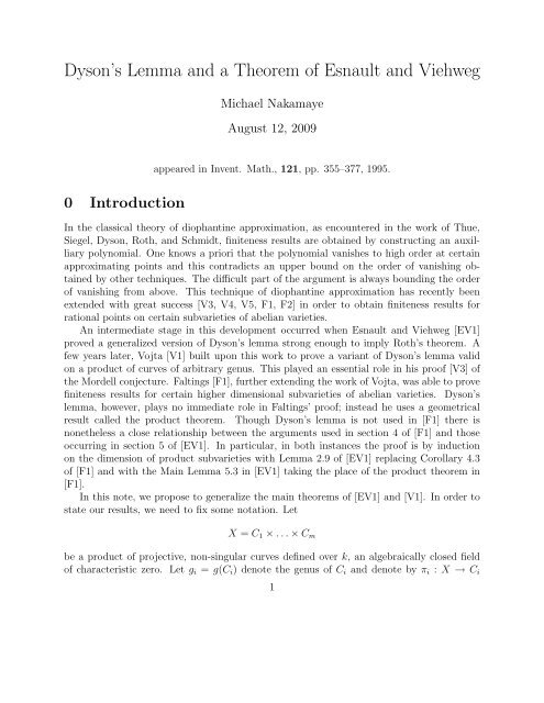
Dyson’s Lemma and a Theorem of Esnault and ViehwegMichael NakamayeAugust 12, 2009appeared in Invent. Math., 121, pp. 355–377, 1995.0 IntroductionIn the classical theory of diophantine approximation, as encountered in the work of Thue,Siegel, Dyson, Roth, and Schmidt, finiteness results are obtained by constructing an auxilliarypolynomial. One knows a priori that the polynomial vanishes to high order at certainapproximating points and this contradicts an upper bound on the order of vanishing obtainedby other techniques. The difficult part of the argument is always bounding the orderof vanishing from above. This technique of diophantine approximation has recently beenextended with great success [V3, V4, V5, F1, F2] in order to obtain finiteness results forrational points on certain subvarieties of abelian varieties.An intermediate stage in this development occurred when Esnault and Viehweg [EV1]proved a generalized version of Dyson’s lemma strong enough to imply Roth’s theorem. Afew years later, Vojta [V1] built upon this work to prove a variant of Dyson’s lemma validon a product of curves of arbitrary genus. This played an essential role in his proof [V3] ofthe Mordell conjecture. Faltings [F1], further extending the work of Vojta, was able to provefiniteness results for certain higher dimensional subvarieties of abelian varieties. Dyson’slemma, however, plays no immediate role in Faltings’ proof; instead he uses a geometricalresult called the product theorem. Though Dyson’s lemma is not used in [F1] there isnonetheless a close relationship between the arguments used in section 4 of [F1] and thoseoccurring in section 5 of [EV1]. In particular, in both instances the proof is by inductionon the dimension of product subvarieties with Lemma 2.9 of [EV1] replacing Corollary 4.3of [F1] and with the Main Lemma 5.3 in [EV1] taking the place of the product theorem in[F1].In this note, we propose to generalize the main theorems of [EV1] and [V1]. In order tostate our results, we need to fix some notation. LetX = C 1 × . . . × C mbe a product of projective, non-singular curves defined over k, an algebraically closed fieldof characteristic zero. Let g i = g(C i ) denote the genus of C i and denote by π i : X → C i1

the projection to the i th factor. Let L be an invertible sheaf on X and fix a global sections ∈ H 0 (X, L). We first need to define, following [V1] Definition 0.2 and [EV1] Definition0.2, the index of s at a closed point of X.Definition 0.1 Let s ∈ H 0 (X, L) and let ζ ∈ X be a closed point. Let z j be a localparameter in O πj (ζ),C j. We also denote by z j the induced function on X. Then taking a localtrivialization of L, s has a power series expansion about ζs = ∑ α≥0b α z α 11 · . . . · z αmm , α = (α 1, . . .,α m ).Let a = (a 1 , . . .,a m ) be an m–tuple of non–negative real numbers. Then the index ind a (ζ, s)with respect to a of s at ζ is defined as follows:{ ∣ m}∑ ∣∣∣∣ind a (ζ, s) = min a i α i b α ≠ 0 .i=1It is clear that ind a (ζ, s) does not depend on the choice of the local trivialization of L or onthe choice of local parameters {z j }.Next we define a set of invariants of the sheaf L which measure the “degree” of L in thedifferent directions.Definition 0.2 Let L be an invertible sheaf on X and choose a closed point P i ∈ C i forall i. We define the intersection numberd i (L) := L · [π ∗ 1O C1 (P 1 ) · . . . · π ∗ i−1O Ci−1 (P i−1 ) · π ∗ i+1O Ci+1 (P i+1 ) · . . . · π ∗ mO Cm (P m ) ] .We will usually abbreviate d i = d i (L) and d = (d 1 , . . .,d m ). We also defineδ i = δ i (L) :=m∑j=i+1d j and δ = δ(L) := (δ 1 , . . .,δ m ).Note that if D is a Q–Cartier divisor on X, d(D) still makes since the invariant d is definedin terms of intersection numbers. Finally for any divisors D i on C i with deg D i = d i writem⊗F d := πi ∗ O C i(D i ).i=1Of course F d depends on the choice of the divisors D i but as we will only be concerned withits numerical equivalence class we abuse notation and suppress this dependence.Having defined the index, we need to define an associated volume which measures howmany linear conditions are imposed on a function f ∈ O ζ,X in order to satisfy ind a (ζ, f) ≥ t.We copy [EV1] Definition 0.2:Definition 0.3 Let I n = {(ξ ν ) ∈ R n ; 0 ≤ ξ ν ≤ 1} and let{}m∑I(d, a, t) = (ξ ν ) ∈ I n ; d ν ξ ν a ν ≤ t .2ν=1

Then define∫Vol(d, a, t) :=I(d,a,t)dξ 1 ∧ . . . ∧ dξ m .One sees that Vol(d, a, t) is the asymptotic proportion of total conditions imposed on apolynomial P of degree ≤ (nd 1 , . . .,nd m ) in order to have index ≥ nt at a fixed point in X(for n → ∞). We can now state the main theorem of this paper:Theorem 0.4 Let S = {ζ 1 , . . .,ζ M } ⊂ X be a finite subset such that card(S) = card[π j (S)]for all j. LetM i = max{2g i − 2 + M, 0}.Let D be a numerically effective Q–Cartier divisor with d(D) ≤ d = d(L) such that thereexists N > 0 for which [ (L(D) ) ]h 0 ⊗ F⊗−1 ⊗Nd ≠ 0.Let P i ∈ C i be a fixed closed point. Let s ∈ H 0 (X, L) and suppose t i = ind a (ζ i , s). Then(∏ m)∑ Md i Vol(d, a, t i ) ≤ 1 [L(D) ⊗i=1 i=1m!( m−1 ⊗i=1π ∗ i O Ci (δ i M i · P i ))] top,where the exponent top means the highest power of self-intersection.In qualitative language, Theorem 0.4 states that for n large the linear conditions imposedon a section s ∈ H 0 (X, L ⊗n ) in order to satisfy ind a (ζ i , s) ≥ t i are “almost independent.”The failure for the conditions to be independent is measured by the perturbation termO X (D) ⊗ m−1i=1 πi ∗ O Ci (δ i M i · P i ) and the perturbation is “small” when for example D is nottoo positive and d i ≫ d i+1 for all i. To see this consider [EV1] Theorem 0.4:Corollary 0.5 (Esnault–Viehweg) With notation as in Theorem 0.4 suppose X = (P 1 ) mis a product of m projective lines and L = ⊗ mi=1 π ∗ i O P 1(d i). Letting M ′ = max{M − 2, 0},⎛M∑m−1 ∏Vol(d, a, t i ) ≤i=1i=1⎝1 + M ′m ∑j=i+1⎞d j⎠.d iFor the proof of Corollary 0.5, note that when X is a product of projective lines Definition0.2 implies that L ≃ F d and consequently one can take D = 0 in Theorem 0.4. A slightlyweaker version of [V1] Theorem 0.4 also follows from Theorem 0.4 or rather from its proof:Corollary 0.6 (Vojta) Let X = C 1 ×C 2 be a product of two smooth projective curves. Lets ∈ H 0 (X, L) and let e denote the maximum multiplicity of all non-fibral components of thezero scheme Z(s). ThenM∑Vol(d, a, t i ) ≤ L · L + eM 1′ .2d 1 d 2 d 1 d 2i=13

Corollary 0.6 will follow readily from the general method used to tackle Theorem 0.4.Vojta’s result [V1] is better by a factor of two on the second term on the right; for an analysisof this situation, see [EV1] §10.The drawback with Theorem 0.4 is the dependence on the Q-divisor D. It is not clear,given an arbitrary line bundle L on X, how to compute the “best” or minimal D. In someinstances, however, such as the line bundles used by Faltings [F1] and Vojta [V4], one hascontrol over D and it would perhaps be interesting to carry out the proof of the Mordellconjecture in [V4] using Theorem 0.4.Our proof of Theorem 0.4 combines ideas of Esnault and Viehweg [EV1], Vojta [V1], andFaltings [F1]. In broad outline, the proof follows [EV1] §1 – §5 very closely. In particular,we derive Theorem 0.4 from the positivity of a certain sheaf constructed from L and thepositivity statement is shown by induction on the dimension of product subvarieties. But ourconstruction is more direct in that instead of working with weak positivity of direct imagesheaves we take “derivatives” of the section s and use a result resembling Faltings’ ProductTheorem. Most of the results of [EV1] §1 – §5 carry over to the more general setting withlittle or no modification. An exception, however, is [EV1] §2 where the proofs, relying onexplicit constructions of multihomogeneous polynomials, need to be replaced with somewhatmore abstract methods. In particular, the Q–divisor D in the statement of Theorem 0.4 isnecessary in order to derive the analogue of [EV1] Lemma 2.9 (ii).In simplifying the logic of the proof, we hope to make the more technical sections of [EV1]available to a wider audience. A fundamental insight of [EV1], exploited most fully by Vojta[V1, V2, V3], is that lower bounds on vanishing come from arithmetic conditions while theupper bounds are purely geometric. The full significance of the methods of weakly positivesheaves and their relation to diophantine problems have not been completely understood. Inparticular, one might hope to use weak positivity in order to give a more “geometric” proofof the results in [F2].The stucture of the paper is as follows. In order to prove Theorem 0.4 it suffices to showthat a certain sheaf is positive; in practice, this means producing more sections s ′ ∈ H 0 (X, L)with index at least t i at ζ i . If there were enough such sections to generate L off of the pointsζ i , Theorem 0.4 would follow immediately. In full generality, however, s might be the onlyglobal section of L with index at least t i at ζ i . In order to produce more sections, we takederivatives of s. This is straightforward in the case when X is a product of projective linesbut in general more care is necessary and we introduce the necessary definitions in section 1.In section 2 we show, following [EV1] §5, how to deduce Theorem 0.4 from the positivity ofan invertible sheaf. The positivity result is shown in two steps, occupying sections 3 and 4respectively. First one shows that after taking a “bounded” number of derivatives of s, theextra sections generate except on a finite union of proper product subvarieties. This allowsone to induct on the dimension of X and the inductive step is carried out in section 4. Atthe end of section 4 we show how to derive Vojta’s result [V1] with the techniques developedto prove Theorem 0.4.Acknowledgments.This paper forms part of my Ph.D. thesis and it is a pleasure to thank my advisor Serge4

Lang for his encouragement and guidance. I would also like to thank H. Esnault, E. Viehweg,P. Vojta, and especially R. Lazarsfeld for many stimulating conversations without which thiswork could not have been completed.Notation and Conventions• On a variety X, a Q-Cartier divisor is an element of Div(X) ⊗Q where Div(X) is thegroup of Cartier divisors on X.• A Q-Cartier divisor on X is said to be numerically effective or nef for short if D·C ≥ 0for all integral curves C ⊂ X (of course the product D·C is just the intersection producton Cartier divisors and is extended by linearity to Div(X) ⊗ Q).• If F is a coherent sheaf on X then h i (X, F) = dim H i (X, F).• When X is smooth K X denotes the canonical bundle on X.• If f : X → Y is a morphism of schemes and I is an ideal sheaf on Y , then we writef −1 I for the inverse image ideal sheaf on X (cf. [H] p. 163).1 PreliminariesAs in the introduction, fix once and for all a product of smooth projective curvesX = C 1 × . . . × C m .An important special case (the case handled by [EV1]), which we will consider in some depthas it has the advantage of being very concrete, is that of a product of m projective lines:LetP = P 1 1 × . . . × P1 m .R = k[X 1 , Y 1 , . . .,X m , Y m ]denote the projective coordinate ring of P. If I ⊂ R is a homogeneous ideal, then denoteby V (I) ⊂ P the associated subscheme and by Z(I) = V (I) red the underlying point set. Wewill often work on a fixed product affine open subset A = ∏ mi=1 A 1 i ⊂ P where each A 1 i isgiven by, say, Y i ≠ 0. Let ξ i denote the affine coordinate on A 1 i . For an m–tuple of integersd = (d 1 , . . .,d m ) writem⊗O P (d) = πi ∗ O P 1(d i).ii=1In what follows we will not distinguish between a global section P ∈ H 0 [O P (d)] and theassociated polynomial in several variables P A .5

Dyson’s Lemma can be viewed as a statement about certain derivatives of sections of linebundles. In the case of P it is clear how to take derivatives of the polynomial P(ξ 1 , . . .,ξ m ).To fix notation, let D i = ∂/∂ξ i andD α =m∏i=1D α ii , for an m–tuple α = (α 1 , . . .,α m ).It will be helpful in some instances not only to take derivatives locally on A but also globally.If s ∈ H 0 [P, O P (d)] and Z ⊂ Z(s) is some integral subvariety contained in the zero schemeof s, then one can define D i (s) as a meromorphic section of O P (d) ⊗ πi ∗K P 1 |Z: locally, oniA say, D i (s) is given by taking the derivative in the naive sense of polynomials. In practice,however, it will be necessary to have an everywhere regular section of O P (d) ⊗πi ∗K P 1 |Z andiso a slight modification will be necessary; we will describe this modification at the end ofthe section.The notion of partial derivatives can now be extended to products of curves of arbitrarygenus (cf. [F1] p. 560 and p. 566 for a more general treatment). Fix projective embeddingsC i ֒→ P n iand generic projections p i : C i → P 1 . Then one can pull back the derivation onP 1 via p i , with poles along the ramification divisor R of p i and so obtain:Definition 1.1 Let s ∈ H 0 (X, L) and suppose Z ⊂ Z(s). Then D i (s)|Z is the meromorphicsection of L[π ∗ i (p ∗ iK P 1 +R)]|Z ≃ L(π ∗ i K Ci )|Z obtained locally by pulling back the derivationon O P 1 via the composition p i · π i . Higher order derivatives are defined analogously so forα = (α 1 , . . .,α m )( m)∣D α ∑ ∣∣∣∣(s) is a meromorphic section of L α i πi ∗ K C iZi=iprovided all partial derivatives D β (s) with β < α vanish identically along Z.Having defined derivatives we can reformulate Definition 0.1. For s ∈ H 0 (X, L) and aclosed point ζ ∈ X we have{ m∣ }∑ ∣∣∣∣ m∏ind a (ζ, s) = min a i α i D α (s)|ζ ≠ 0 where D α = D α ii .i=1i=1When X = P and L = O P (d), ind a (ζ, s) ≥ t if and only if s has a zero of type (a, t) at ζ inthe language of [EV1] Definition 0.2.Fix a finite set of points S = {ζ i } M i=1 ⊂ X and an m–tuple a = (a 1 , . . .,a m ) as inDefinition 0.1. We want to define an ideal sheaf I(s) on X so that s ∈ H 0 [X, L ⊗ I(s)] andso that I(s) characterizes the index of s at the points ζ i ∈ S. For a fixed point ζ ∈ X andt ∈ R + , define an ideal sheaf I ζ,d,t as follows: write ζ j = π j (ζ) and consider the local ringm⊗O ζ,X ≃ O ζj ,C j.j=16

Let z j be a local parameter in O ζj ,C jso that {z 1 , . . .,z m } form a regular system of parametersfor O ζ,X . First we define an ideal I ζ,d,t ⊂ O ζ,X :⎛⎞m∏I ζ,d,t := ⎝M α = z α jjα j ≤ d j for all j and ind a (ζ, M α ) ≥ t⎠.∣j=1The definition of I ζ,d,t does not depend on the choice of local parameters {z 1 , . . .,z m }. AlthoughI ζ,d,t does depend on the choice of a used to define the index, we omit this from thenotation as a will be fixed throughout. Choose a small product affine open subsetm∏U = U j = Specj=1m⊗A jj=1with z i ∈ A i for all i so that the only zero of z i in U i is ζ i . We will continue to denote by I ζ,d,tthe ideal sheaf on U associated to I ζ,d,t . Letting f : U ֒→ X denote the natural inclusion,defineI ζ,d,t := f ∗ I ζ,d,t ∩ O X (cf. [EV1] 2.2).It is not difficult to check that the definition does not depend on the choice of U.Definition 1.2 Fix a set S ⊂ X as in Theorem 0.4 and let t i = ind a (ζ i , s). ThenM⋂I(s) := I ζi ,d,t i.i=1It is clear from the definition that s ∈ H 0 [X, L ⊗ I(s)]. In the special case where X = Pand L = O P (d), the sheaf I(s) corresponds with L ′ as defined in [EV1] 2.6. Note also (cf.[EV1] 2.3) that the Riemann–Roch theorem for curves implies thatI ζ,nd,nt ⊗ F ⊗nd is generated by global sections for all n ≫ 0.There is some subtlety here because when t = m, this statement is false for an arbitrarychoice of divisors D i on C i in the definition of F d . The problem is not serious, however,because one can always add the Q–Cartier divisor ǫ ∑ mi=1 π ∗ i D i to O X (D) and F d ; one canthen verify that taking the limit as ǫ → 0 yields Theorem 0.4. We will frequently encounterthis procedure. In any case, we will always have t < m so this is not important.We will need an auxilliary sheaf M(L, S), depending on L and the finite subset S ⊂ X.This will be used to make adjustments after taking derivatives of the section s ∈ H 0 (X, L).WriteS i = π i (S) = {ζ i1 , . . ., ζ iNi }.Also if g(C i ) = 0 and N i = 1 let S i ′ = {ζ i1, ζ i2 } for a general point ζ i2 ∈ C i . Otherwise letS i ′ = S i. Finally set{maxN i ′ {Ni , 2}, if g(C=i ) = 0,N i , otherwise.7

Thus N ′ i = card(S′ i ).Definition 1.3 Given an invertible sheaf L on X, a finite subset S ⊂ X, and an m–tupleα = (α 1 , . . .,α m ), let⎛⎞N m⊗M(L, S, α) := πi∗ ∑i′⎝α i K Ci + α i ζ ij⎠i=1j=1We will abbreviate M(α) = M(L, S, α), the set S and the sheaf L being tacitly understood.Suppose Z ⊂ X is a subvariety for which D α (s)|Z is defined and let j : Z ֒→ X denotethe inclusion. The point of Definition 1.3 is that after adjusting D α (s) by M(α) not onlydoes D α (s) become an everywhere regular section but also one can write⎡⎛ ⎞⎤N m∑′⎣D α (s) + πi∗ ∑i⎝α i ζ ij⎠⎦Z ∈i=1 j=1 ∣ H0 [L ⊗ M(α) ⊗ j −1 I(s)]. (1.4)To see this, identify K Ci with some effective divisor if g(C i ) > 0 or with O P 1(−ζ i1 − ζ i2 ) incase g(C i ) = 0. This makes⎛ ⎞N m∑D α (s) + πi∗ ∑i′ ⎝α i ζ ij⎠Zi=1 j=1 ∣an everywhere regular section of L ⊗ M(α) and one can check locally that this is a sectionof H 0 [L ⊗ M(α) ⊗ j −1 I(s)].2 Reduction to a Positivity StatementIn this section we show how to reduce Theorem 0.4 to a positivity result. First note thatby replacing L with L ⊗n and s with s ⊗n we can assume without loss of generality thatN = 1 in the statement of Theorem 0.4. Choosing n sufficiently divisible will also guaranteethat [EV1] Lemma 1.9 holds. Also, it suffices to prove Theorem 0.4 for rational m–tuplesa = (a 1 , . . .,a m ) and, clearing denominators, one can assume that all a i are integers.Theorem 2.1 Let D and s ∈ H 0 (X, L) be as in the statement of Theorem 0.4. Letτ : ˜X → Xbe the blow-up of X along the ideal sheaf I(s) and let E denote the exceptional divisor.Recall δ = (δ 1 , . . .,δ m ) from Definition 0.2. Then τ ∗ [L(D) ⊗ M(δ)](−E) is nef.8

To show how Theorem 2.1 implies Theorem 0.4 we will need a few technical lemmas.The reader familiar with [EV1] can refer to [EV1] 5.11–5.12 and skip the rest of this sectionexcept for Lemma 2.2 which will be used later in §4.Lemma 2.2 ([EV1] Lemma 2.7) With S ⊂ X, s ∈ H 0 (X, L), and t i as in the statement ofTheorem 0.4, let ζ 1 , ζ 2 ∈ S be two points. Thenm∑a i d i ≥ t 1 + t 2 . (2.2.1)i=1Proof: The proof will be by induction on m and already gives a flavor of the inductivepart of the proof of Theorem 2.1 in §4. Let V = π1 −1 [π 1 (ζ 1 )] and write Z(s) = Z(s ′ ) + aVfor s ′ ∈ H 0 (X, L ′ ) and V ⊄ supp[Z(s ′ )]. Replacing (s, L) by (s ′ , L ′ ) it is clear thatm∑a i d i ≥ t 1 + t 2 if and only ifi=1m∑a i d ′ i ≥ t′ 1 + t′ 2i=1because the change decreases both sides of (2.2.1) by exactly a · a 1 . So we can assume thats|V is a well defined non-zero section of L|V . Let ζ ′ i = π {2,...,m}(ζ i ) for i = 1, 2. It followsthat ind a (ζ ′ 1, s|V ) ≥ t 1 . Thus, Lemma 2.2 will be proven by the inductive hypothesis if wecan show thatind a (ζ ′ 2 , s|V ) ≥ t 2 − a 1 d 1 . (2.2.2)One can clearly assume that t 2 − a 1 d 1 > 0. So suppose (2.2.2) is false. Then there existsa differential operator D α withChoose α so thatD α (s|V )|ζ 2 ′ m ≠ 0, ∑a i α i < t 2 − a 1 d 1 .i=2(a) D β (s) vanishes identically along C 1 × ζ ′ 2 for β < α,(b) D α (s) does not vanish identically along C 1 × ζ 2 ′ ,m∑(c) a i α i < t 2 − a 1 d 1 .i=2Hence D α (s)|C 1 ×ζ ′ 2 gives a well defined non-zero global section of an invertible sheaf on C 1with degree ≤ d 1 . Thus one can find α 1 ≤ d 1 such thatD α 11 [Dα (s)] |ζ 2 ≠ 0and this contradicts the assumption that ind a (ζ 2 , s) ≥ t 2 .9

Corollary 2.3 ([EV1] Lemma 2.8) Let W i be the support of the subscheme defined by I ζi ,s.Then W i⋂ Wj is empty for all i ≠ j.Proof: Corollary 2.3 is a straightforward consequence of Lemma 2.2 and is left as anexercise; the proof in [EV1] Lemma 2.8 goes through unchanged as [EV1] Lemma 2.5 easilyextends to our situation.Since we have assumed N = 1, the assumptions in Theorem 0.4 imply that there is aneffective divisor Γ such thatO X (Γ) ≃ L(D) ⊗ Fd −1 .Lemma 2.4 The invertible sheaf O X (Γ) ⊗ M(δ) is nef.Lemma 2.4 will be proved at the end of §3; it is similar to the proof of Theorem 2.1except that the inductive step is significantly simpler.Lemma 2.5 Let ζ ∈ X be a closed point and let Z ζ,n be the subscheme defined by I ⊗nζ,d,t fort = ind a (ζ, s). Thenh ( 0 X, Z ζ,n ⊗ [L(D) ⊗ M(δ)] ⊗n)limn→∞ n m ∏ m≥ Vol(d, a, t).i=1 d iProof: By [EV1] Lemma 1.9 and the assumption made at the beginning of this sectionBy Definition 0.3 one obtains (cf. [EV1] 2.4)I ⊗nζ,d,t = I ζ,nd,nt⎛ ( )lim ⎝ h0 X, F ( )d⊗n − h0X, Fd ⊗n ⎞⊗ I ζ,nd,ntn→∞n m ∏ ⎠m= Vol(d, a, t).i=1 d iFrom the long exact cohomology sequence associated toone obtainsSince0 → I ζ,nd,nt ⊗ F ⊗nd→ F ⊗nd→ Z ζ,n ⊗ F ⊗nd → 0⎛ ( )lim ⎝ h0 X, Z ζ,n ⊗ Fd⊗n ⎞n→∞ n m ∏ ⎠m≥ Vol(d, a, t). (2.5.1)i=1 d i[L(D) ⊗ M(δ)] ⊗n ≃ [O X (Γ) ⊗ M(δ)] ⊗n ⊗ F ⊗nd .Lemma 2.5 now follows from (2.5.1) and Lemma 2.4 by adding ǫA to L where A is an ampledivisor on X and taking the limit as ǫ → 0.Proof of Theorem 0.4 from Theorem 2.1: first we need to show, in the language of [EV1]Definition 3.3, that the ideal sheaf I(s) is full. This can be done as in [EV1] §3, using the10

covering construction of [V1] Lemma 3.1 instead of the simple ramified cover of P used in[EV1] 3.9. We will not reproduce the argument here. The rest of the argument is purelycohomological and the fact that I(s) is full will be used in order to apply the Leray spectralsequence. The argument is given in [EV1] 5.11–5.12.Let f : Y → ˜X be a desingularization of ˜X and let g = τ · f : Y → X. LetO Y (−F) = Im : g ∗ I(s) → O Y .Then O Y (−F) ≃ f ∗ O ˜X(−E) and so by Theorem 2.1, g ∗ [L(D) ⊗ M(δ)](−F) is nef. Henceby [EV1] Corollary 4.7, it follows that there exists a polynomial P(n) of degree ≤ m − 1such thath 1 ( X, [g ∗ [L(D) ⊗ M(δ)](−F)] ⊗n) ≤ P(n) for all n ≥ 0.Using the fact that I(s) is full and the Leray spectral sequence it follows thath 1 ( X, [L(D) ⊗ M(δ) ⊗ I(s)] ⊗n) ≤ P(n) for all n ≥ 0. (2.6)Suppose Z n ⊂ X is the subscheme defined by the ideal sheaf I(s) ⊗n and consider the exactsequence0 → [L(D) ⊗ M(δ) ⊗ I(s)] ⊗n → [L(D) ⊗ M(δ)] ⊗n → Z n ⊗ [L(D) ⊗ M(δ)] ⊗n → 0. (2.7)By Theorem 2.1, τ ∗ [L(D) ⊗ M(δ)](−E) is nef on ˜X and hence L(D) ⊗ M(δ) is nef on X.Perturbing L by ǫA for a rational ǫ ≪ 1 and taking the limit as ǫ → 0, we can assume thatL(D) ⊗ M(δ) is ample. Thus for n ≫ 0h 0 ( X, [L(D) ⊗ M(δ)] ⊗n) = χ ( [L(D) ⊗ M(δ)] ⊗n) = nmm! [L ⊗ M(δ)]top + O(n m−1 ). (2.8)On the other hand Corollary 2.3 imples that Z n = ⋃ Z ζi ,n is a disjoint union of the subschemesZ ζi ,n defined in Lemma 2.5. From Lemma 2.5 it follows thatlimn→∞⎛⎝ h0 ( Z n ⊗ [L(D) ⊗ M(δ)] ⊗n)n m ∏ mi=1 d i⎞M∑⎠ ≥ Vol(d, a, t i ). (2.9)i=1Now it follows from (2.6), (2.8), (2.9), and the long exact cohomology sequence associatedto (2.7) thatM∑ [L(D) ⊗ M(δ)]topVol(d, a, t i ) ≤ ,m!i=1and Definition 1.3 finishes the proof of Theorem 0.4 from Theorem 2.1.11

One also sees thatLetZ ( D α (P), D 1 m [Dα (P)], . . ., D dmm [Dα (P)] ) = Z [A α,0 (ξ), . . ., A α,dm (ξ)]. (3.6)⎛⎧⎨J ′ = ⎝⎩ Dα [A 0,i (ξ 1 , . . .,ξ m−1 )]0 ≤ i ≤ d m and 0 ≤ α i ≤∣It follows from (3.4), (3.5), (3.6), and the definition of J thatV ⊂ Z(J ′ ) ⊂ proper product subvariety,with the last inclusion following from the inductive hypothesis.m−1 ∑⎫⎬d j⎭j=i+1Next we prove Lemma 3.3. For this we need the following easy result:Lemma 3.7 Let η denote a general closed point of V . There exists a regular system ofparameters {Q i (ξ)} r i=1 for O V,A and differential operators {∆ i } r i=1 satisfying the followingProof: Let(i)∆ i Q j (η) = δ ij , δ ij the Kronecker symbol,(ii) ∆ i = D ci ,(iii) 1 ≤ c 1 < . . . < c r ≤ m − 1.T η V ⊂ T η A ≃ C m = C 1 × . . . × C mdenote the tangent space of V at η. Since π m : V → A 1 m is surjective it follows thatπ m : T η V → C m is surjective. Hence we haveT η V + < ∂/∂ξ 1 , . . .,∂/∂ξ m−1 >= T η A,and Lemma 3.7 is then a linear algebra exercise.LetFor any D α (P) ∈ J one can writer∏Q α (ξ) = Q α i(ξ), α = (α 1 , . . .,α r ),i=1r∏∆ α = ∆ α ii , α = (α 1 , . . .,α r ).i=1⎞⎠.D α P(ξ) = ∑ βu α,β (ξ)Q β (ξ) where u α,β (ξ) = 0 or u α,β (η) ≠ 0, ∞.Letκ = min {|β| : u α,β (ξ) ≠ 0}.13

In order to prove Lemma 3.3 it will suffice to show that κ > d m . Suppose that this is notthe case. Then we can choose D α (P) ∈ J withD α (P) = ∑ u α,β (ξ)Q β (ξ), u α,β (η) ≠ 0, ∞, and |β| ≤ d m .Take D α (P) and β as above with |β| minimal. Then by (i) of Lemma 3.7 we see that∆ β [D α (P)](η) ≠ 0. But by (ii) and (iii) of Lemma 3.7 and the assumption that |β| ≤ d mwe see that ∆ β [D α (P)] ∈ I, a contradiction. Thus κ > d m .The proof of Theorem 3.1 follows precisely the same model. Let η be a general point ofC. Since Theorem 3.1 is local we can restrict to a small affine open subset U ⊂ X containingη; thus we can assume that the derivatives D α (s) are globally defined and that s can beidentified, via a local trivialization of L, with a function P s on U. By abuse of notation, westill denote by C the intersection C ∩ U and similarly the domain of all projections will betacitly assumed to be restricted to U. The argument of Lemma 3.3 goes through unchanged,yieldingWe claim thatD α (P s ) ∈ P dm+1C , for all 0 ≤ α i ≤m−1 ∑j=i+1[π −1{1,...,m−1} π{1,...,m−1} (C) ] ⊂ Z[D α (P s )] for all 0 ≤ α i ≤d j . (3.8)m−1 ∑j=i+1d j . (3.9)If (3.9) did not hold then there would exist a point P ∈ π {1,...,m−1} (C) and a multi–index αas in (3.9) such that D α ∣(P s ) ∣π −1 (P) is a local equation for a non–zero global section{1,...,m−1}of the sheaf L|P × C m . But (3.8) says that D α (P s ) ∣ ∣ ∣π−1{1,...,m−1} (P) has multiplicity ≥ d m + 1at at least one point and this contradicts Definition 0.2. Now choose a generic η ∈ C m sothat s|C 1 × · · · × C m−1 × η is a non-zero section of L|C 1 × · · · × C m−1 × η. By (3.9)π {1,...,m−1} (C) ⊂ Z ( D α [ P s |π −1m (η)]) for all 0 ≤ α i ≤m−1 ∑d jj=i+1and Theorem 3.1 follows by induction on m (since π {1,...,m−1} (C) is not contained in a properproduct subvariety).As a corollary of Theorem 3.1 we derive a rough analogue of [EV1] 5.5:Corollary 3.10 Suppose C ⊂ X is not contained in a proper product subvariety. Let j :C ֒→ X denote the natural inclusion. Then for α ≥ δ there exists a global section σ ∈H 0 [C, L ⊗ M(α) ⊗ j −1 I(s)].Proof: Theorem 3.1 states that there is an α ≤ δ such that the meromorphic sectionD α (s)|C is non-zero. Since D α (s)|C is non-zero, (1.4) shows thath 0 [C, L ⊗ M(α) ⊗ j −1 I(s)] ≠ 0,and increasing α does not effect the conclusion of Corollary 3.10.In the special case X = P and L = O P (d) Corollary 3.10 has a more explicit statementand proof:14

Corollary 3.11 Let {ζ i } i∈S be a finite collection of points in P and suppose there existsP ∈ H 0 [P, O P (d)] with a zero of type (a, t i ) at ζ i . ThenI(s) ⊗ O P (d ′ 1 , . . .,d′ m )is generated by global sections on some product open subset ford ′ i ≥ d i + N ′ i δ i.Proof: By applying a projective linear automorphism to P we can assume without lossof generality that ζ i1 = (0, 1) and ζ i2 = (1, 0) for all i (notation as in Definition 1.3). Let⎛⎧⎨I ′ = ⎝⎩ Dα (P) · ξ α ·m−1 ∏ ∏N ′(ξ i − ζ ij ) α m−1 ∏ii=1 j=3 ∣ ξα =i=1ξ α ii⎞⎫⎬and 0 ≤ α i ≤ δ i⎠.⎭Here the derivatives are taken in the naive sense on A. By construction, the generators ofI ′ all have zeroes of type (a, t i ) at ζ i . Also I ′ is generated by polynomials of multidegree≤ (d 1 + N ′ 1δ 1 , . . ., d m + N ′ mδ m ). Moreover, by constructionZ(I ′ ) ⊂ Z(I) ⋃ i,jm−1 ⋃Z(ξ i − ζ ij ) Z(ξ i ).i=1Corollary 3.2 says that Z(I) is contained in a finite union of product subvarieties and thisconcludes the proof of Corollary 3.11.Next we derive the precise equivalent of [EV1] 5.5 from Corollary 3.10.Lemma 3.12 Let τ : ˜X → X be the blow-up of X along I(s) with exceptional divisor E andlet α = (α 1 , . . .,α m ) ≥ (δ 1 , . . .,δ m ) be as in Corollary 3.10. Suppose ˜C ⊂ ˜X and C = τ( ˜C)is not contained in a proper product subvariety. Thenτ ∗ [L ⊗ M(α)](−E) · ˜C ≥ 0.Proof: Since τ ∗ M(α − δ) is nef, it suffices to show that τ ∗ [L ⊗ M(δ)] · ˜C ≥ 0. In thespecial case where X = P, note that the birational morphism τ : ˜P → P is an isomorphismover a product open subset. Thus the global sections guaranteed by Corollary 3.11 lift toglobal sections of τ ∗ [L ⊗ M(δ)](−E) and still generate over some product open subset. Inthe general case, we need to show thatdeg (L ⊗ M(δ)|C) ≥ E · ˜C.By Corollary 3.10 there exists a non-zero section σ ∈ H 0 [C, L ⊗ M(δ) ⊗ j −1 I(s)]. Letg : C ′ → C denote the normalization of C and h = j · g : C ′ → X. Theng ∗ σ ∈ H 0 ( C ′ , g ∗ [L ⊗ M(δ)] ⊗ h −1 I(s) ) .15

Since h −1 I(s) is an invertible sheafand sodeg g ∗ [L ⊗ M(δ)] ≥ deg h −1 I(s).deg [L ⊗ M(δ)] = deg [g ∗ L ⊗ M(δ)] ≥ deg h −1 I(s) = E · ˜C.and Lemma 3.12 follows.Note that in the proof of Lemma 3.12 only M(δ) is needed; the additional twist byO X (D) is only required in the inductive step and in some instances (e.g. the cases of [EV1]and [V1]) this is not necessary. Lemma 3.12 holds also for the blow-up of X along any idealsheaf containing I(s). We also remark that if s 1 ∈ H 0 (X, L 1 ), s 2 ∈ H 0 (X, L 2 ), and s 2 |C isnon-zero for all C ⊂ X not contained in a proper product subvariety, then Theorem 3.1 andLemma 3.12 hold for s 1 ⊗ s 2 ∈ H 0 (X, L 1 ⊗ L 2 ) with δ(L 1 ) in place of δ(L 1 ⊗ L 2 ).We conclude this section by proving Lemma 2.4. If Y ⊂ X is a proper product subvariety,then O X (Γ)|Y is still effective, as one can see by successively restricting to a chain of divisors,each a product subvariety of XX ⊃ D 1 ⊃ . . . ⊃ D r = Y.Thus one can apply Theorem 3.1 and the comments after Definition 1.3 to all proper productsubvarieties Y and any global section of O X (Γ)|Y . A stronger statement than Lemma 2.4acutally holds as the ideal sheaf I(s) is irrelevant for the numerical statement on X andconseqently one only needs to adjust the derivatives enough to make them everywhere regularglobal sections.4 The Inductive StepIn this section we complete the proof of Theorem 2.1. Continue to denote by τ : ˜X → Xthe blow-up of X along I(s) with exceptional divisor E. By Lemma 3.12τ ∗ [L(D) ⊗ M(α)](−E) · ˜C ≥ τ ∗ [L ⊗ M(α)](−E) · ˜C ≥ 0for any curve ˜C ⊂ ˜X such that τ(C) is not contained in a proper product subvariety. At theother extreme, since O ˜X(−E) is τ–ample one automatically has thatτ ∗ [L(D) ⊗ M(δ)](−E) · ˜C > 0 for any curve ˜C contracted by τ.In this section, we prove the the inductive step of Theorem 2.1 which eliminates the casewhen τ( ˜C) is a curve contained in a proper product subvariety. This step occurs in [EV1]5.9–5.10 and our proof will be similar.Case 1 (cf. [EV1] 5.9): the first and easier case is when, using the notation of Corollary2.3, τ( ˜C) ⊂ W i for some i. By Corollary 2.3, this implies that τ( ˜C) ∩ W j is empty for allj ≠ i. LetO ˜X(−F) = Im : τ ∗ I ζi ,d,t i→ O ˜X.16

ThenButτ ∗ [L(D) ⊗ M(δ)](−E) · ˜C = τ ∗ [L(D) ⊗ M(δ)](−F) · ˜C.τ ∗ [L(D) ⊗ M(δ)](−F) ≃ τ ∗ [O X (Γ) ⊗ M(δ)] ⊗ τ ∗ F d (−F).By Lemma 2.4 τ ∗ [O X (Γ) ⊗ M(δ)] is nef and by the comments after Definition 1.2 so isτ ∗ F d (−F). This concludes the proof of Theorem 2.1 in Case 1.Case 2 (cf. [EV1] 5.10): suppose τ( ˜C) ⊄ W i for any i so that j −1 I(s) ≠ 0. Here we willuse the following Lemma:Lemma 4.1 Let P i1 ∈ C i1 , . . ., P ik ∈ C ik be fixed closed points; for simplicity we will assumethat i j = j. LetV k = π −1{1,...,k} (P 1 × . . . × P k )and let f k : V k ֒→ X denote the standard inclusion. For N ≫ 0 and sufficiently divisiblethere exist invertible sheaves L 1 , L 2 on V k with global sections σ 1 and σ 2 respectively suchthat(i)(ii)d(L 1 ) ≤ N · d(L),σ 2 |C ≠ 0 for any curve C not contained in a proper product subvariety,(iii) σ 1 ⊗ σ 2 ∈ H 0 ( V k , L(bD) ⊗N ⊗ f −1k I(s)⊗N) , 0 ≤ b ≤ 1.Proof of Case 2 from Lemma 4.1: given C not contained in any W i , let V k ⊂ X be aproper product subvariety containing C such that C is not contained in a smaller productsubvariety. Consider the following commutative diagram:¯τṼ k❄˜f k✲˜XτV kf k✲❄XHere ¯τ : Ṽ k → V k is the blow-up of V k along the inverse image ideal sheaf f −1k I(s). If Ēdenotes the exceptional divisor of ¯τ then by [Fu] Appendix B 6.9, E|Ṽk = Ē. Henceτ ∗ [L(bD) ⊗ M(δ)](−E)|Ṽk ≃ ¯τ ∗ [L(bD) ⊗ M(δ)|V k ](−Ē). (4.2)Let σ 1 ⊗ σ 2 ∈ H ( 0 L(bD) ⊗N ⊗ f −1k I(s)⊗N) be the section guaranteed by Lemma 4.1. Onecan then apply the comment following Lemma 3.12 to σ 1 ⊗ σ 2 to conlude, using (4.2), thatτ ∗ [L(bD) ⊗ M(δ)](−E) · ˜C ≥ 0.But O X (D) is nef and b ≤ 1 so this finishes the proof of Case 2 and of Theorem 2.1.17

Two ingredients are needed to prove Lemma 4.1: first an analysis of fk−1 I(s) and secondan analysis of L|V k . In the case where X = P the reader can find an explicit statement andproof of both steps in [EV1] Lemma 2.9.Lemma 4.3 (cf. [EV1] Lemma 2.9i) Let T i = {j : P j ≠ π j (ζ i )} with notation as in Lemma4.1 and write⎧⎫⎨τ i = max⎩ t i − ∑ ⎬a j d j , 0⎭ , 1 ≤ i ≤ M.j∈T iLet ζ ′ i = π {k+1,...,m}(ζ i ) and let d ′ = (d k+1 , . . .,d m ). Thenf −1k [I(s)] = ⋂I ζ ′i ,d ′ ,τ ii∈SProof: This can be shown by direct computation as in [EV1] Lemma 2.9 (i) by consideringgenerators of I ζi ,d,t i.Lemma 4.4 Using the notation of Lemma 4.1, write Z(s) = Z(s 1 ) + β 1 V 1 such that V 1 ⊄supp[Z(s 1 )] and inductivelyAlso writeZ(s i |V i ) = Z(s i+1 ) + β i+1 V i+1 with V i+1 ⊄ supp[Z(s i+1 )].t ′ i = ind a (ζ ′ i, s k |V k ).Then τ i > t ′ i for at most one i. Moreover, in this case if e = τ i − t ′ i > 0 then for all j ≠ ieither τ j = 0 or t ′ j − τ j ≥ e.Proof: One can directly verify, following the method of Lemma 2.2, that⎧ ⎫⎨t ′ j ≥ max ⎩ t j − ∑ a i d i + ∑a i β i − ∑ ⎬a i β i , 0 , 1 ≤ j ≤ M. (4.4.1)⎭i∈T j i∈T j i∉T jFor all inidices j for which T j = {1, . . .,k} it is clear that t ′ j ≥ τ j and that if τ j ≠ 0 thent ′ j − τ j =m∑i=k+1a i β i ≥ e,the last inequality following from (4.4.1) and Lemma 4.3. So suppose T j ≠ {1, . . .,k} andτ j > 0. For simplicity of notation, we assume that j = 2 and that τ 1 − t ′ 1 = e > 0. Then⎛⎞2∑ 2∑ 2∑t ′ k ≥ τ k + ⎝ ∑a i β i − ∑a i β i⎠k=1 k=1 k=1 i∈T k i∉T k18

But because card(S) = card[π j (S)] for all j, each index i can fail to be in at most one of T 1 ,T 2 . Thus the big sum on the right hand side is positive and this proves Lemma 4.4.Proof of Lemma 4.1: Lemma 4.4 gives a non-zero section(s k ∈ H 0 V k , L ⊗ ⋂ )I ζi ,d ′ ,t ′ .ii∈SLemma 4.4 also allows one to “perturb” s k into the desired section since τ i and t ′ i differ ina suitably bounded fashion. There are two possibilities. First, one might have τ i = 0 for allbut possibly one i. Since τ i ≤ ∑ mi=k+1 a i d i by Lemma 2.2, there is no trouble in this case,and one can even take N = 1. So suppose that τ i > 0 for at least two indices i and thatτ 1 − t ′ 1 = e > 0. Choose integers N 1, N 2 > 0 such thatN 1 t ′ 1 + N 2m ∑i=k+1a i d i = (N 1 + N 2 )τ 1 .The fact that both N 1 and N 2 can be chosen to be positive follows from Lemma 2.2. Rewritingthis expression givesAn application of Lemma 2.2 givesN 1 e + N 2 τ 1 = N 2m ∑i=k+1a i d i .N 1 e ≥ N 2 τ i for all i ≠ 1. (4.5)Suppose now that i ≠ 1 is an index for which τ i > 0. By Lemma 4.4,N 1 t ′ i ≥ N 1τ i + N 1 e ≥ (N 1 + N 2 )τ i , (4.6)the second inequality following from (4.5).Choose N = N 1 + N 2 and choose F d so that there is a global section ρ ∈ H 0 (V k , fk ∗F d)with ind a (ζ 1, ′ ρ) = ∑ mi=k+1 a i d i . Fix a global section γ ∈ H 0 [X, O X (Γ)] and letσ 1 = s ⊗N 1k ⊗ γ ⊗N 2∈ H 0 (V k , L 1 ), L 1 := fk∗σ 2 = ρ ⊗N 2∈ H 0 (V k , L 2 ), L 2 := fk ∗ F ⊗N 2(L⊗N 1⊗ O X (N 2 Γ) ) ,One verifies from the definitions that (i) and (ii) are satisfied. Let b = N 2 /N. Then sinceL(bD) ⊗N ≃ F d (Γ) ⊗N 2⊗ L ⊗N 1.d .we see that (iii) is satisfied. By the choice of N 1 and N 2 and (4.6) it follows thatand this concludes the proof of Lemma 4.1.σ 1 ⊗ σ 2 ∈ H ( 0 L(bD) ⊗N ⊗ fk−1 I(s)⊗N)We end this section by showing how the methods developed here give a natural proof ofCorollary 0.6 and give some indication of why the case of a surface is significantly simplerthan a higher dimensional variety; the proof of Corollary 0.6 is similar to [EV1] Theorem10.4.19

Lemma 4.7 Let X = C 1 × C 2 with s ∈ H 0 (X, L). Let τ : ˜X → X be the blow-up of Xalong I(s). Then τ ∗ [L ⊗ π ∗ 1(eN ′ 1 · P 1 )](−E) is nef.Proof: the same method used in the general case can be adapted easily to prove Lemma4.7. However, we present a slightly different proof using the following result which in anycase will be needed in order to prove the analogue of Theorem 2.1:Lemma 4.8 Fix a set S ⊂ C 1 ×C 2 and s ∈ H 0 (C 1 ×C 2 , L) as in the statement of Theorem0.4. Then there exists an invertible sheaf G and a section s ′ ∈ H 0 (C 1 × C 2 , L ′ ) such that(i) L ≃ L ′ ⊗ G,(ii) I(s) ≃ I(s ′ ) ⊗ G −1 ,(iii) ind a (ζ i , s ′ ) ≤ min{a 1 d ′ 1 , a 2d ′ 2 }Proof: If t i ≤ min{a 1 d 1 , a 2 , d 2 } for all i then take G = O X . Otherwise let J i be theintersection of all isolated primary components of I ζi ,d,t iand let J i be the associtated idealsheaf on X with zero scheme Y i . Thus Y i is just a union of those fibres of the first andsecond projection along which a polynomial of degree ≤ d and index ≥ t i at ζ i must vanish;in particular, for t i ≤ min{a 1 d 1 , a 2 d 2 }, Y i is empty. Using Lemma 2.2 one can check thatM∑Z(s) = D + Y i ,i=1for an effective divisor D and that D has index ≤ min{a 1 d 1 [O X (D)], a 2 d 2 [O X (D)]} at all ζ i .Taking G = O X( ∑Mi=1Y i)and L ′ = O X (D) concludes the proof of Lemma 4.8.Proof of Lemma 4.7: The argument of §3 easily shows that for C = τ( ˜C) not containedin a proper product subvariety,τ ∗ [L ⊗ π ∗ 1 (eN ′ 1 · P 1)](−E) · ˜C ≥ 0.The remaining case is when C is a fibre of one of the two projections and here we will reduceto proving Lemma 4.7 for s ′ ∈ H 0 (X, L ′ ). With notation as in Lemma 4.8, let τ ′ : ˜X′ → Xbe the blow-up of X along I(s ′ ) with exceptional divisor E ′ . Since I(s) and I(s ′ ) differ byan invertible sheaf, it is well known (cf. [Ha] chapter II, Lemma 7.9) that ˜X and ˜X ′ arecanonically isomorphic. Moreover, if φ : ˜X → ˜X′ denotes the canonical isomporphism thenagain by [Ha] chapter II, Lemma 7.9,It follows thatO(−E) ≃ φ ∗ [O(−E ′ ) ⊗ G −1 ]τ ∗ L(−E) ≃ φ ∗ [τ ′ ∗ (L(−E ′ ) ⊗ G −1 )] ≃ φ ∗ [τ ∗ L ′ (−E ′ )].One then verifies directly that{E ′ · ˜C d′≤ 1 if C is a fibre of the second projectionif C is a fibre of the first projection,d ′ 220

and Definition 0.2 concludes the proof of Lemma 4.7.We also prove Corollary 0.6 first for s ′ ∈ H 0 (X, L ′ ) and then for s ∈ H 0 (X, L); Vojta[V1] argues in a similar fashion using [V1] Theorem 0.4 B to reduce to the case where Z(s)contains no fibres of either projection. Using the notation of §2, consider the exact sequence0 → [L ′ (eN ′ 1 π∗ 1 P 1) ⊗ I(s ′ )] ⊗n → [L ′ (eN ′ 1 π∗ 1 P 1)] ⊗n → Z ′ n ⊗ [L′ (eN ′ 1 π∗ 1 P 1)] ⊗n → 0.Lemma 4.8 implies that Z n ′ is a disjoint union of skyscraper sheaves supported on the pointsζ i . A direct calculation (cf. [EV1] 2.4) givesh ( )0 O Z ′ nlim ≥n→∞ n 2 d 1 d 2M∑Vol(d, a, t ′ i)i=1and the rest of the argument proceeds as in §2.In order to derive the corresponding result for s ∈ H 0 (X, L) it will suffice to show thath ( 0 Z n ⊗ [L(eN 1 ′limπ∗ 1 P 1)] ⊗n)≥n→∞ n 2 d 1 d 2M∑Vol(d, a, t i ),i=1and by Corollary 2.3 we can assume that M = 1. By Lemma 4.8 and the exact sequencewe see that0 → [L(eN ′ 1 π∗ 1 P 1) ⊗ I(s)] ⊗n → [L(eN ′ 1 π∗ 1 P 1)] ⊗n → Z n ⊗ [L(eN ′ 1 π∗ 1 P 1)] ⊗n → 0,h 0 ( Z n ⊗ [L(eN ′ 1 π∗ 1 P 1)] ⊗n) ≥ h 0 ( [L(eN ′ 1 π∗ 1 P 1)] ⊗n) − h 0 ( [L ′ (eN ′ 1 π∗ 1 P 1) ⊗ I(s ′ )] ⊗n) .Now n 2 · Vol(d, a, t) is asymtotically equal to the total number of monomials of degree ≤ ndwith index ≥ nt i at ζ i . Each of these monomials M can be written uniquely as M = f · gwith f ∈ J i and g a monomial of multidegree ≤ d(L ′ ) and index ≥ t ′ i at ζ i . From the previousanalysis of the case for s ′ and the above exact sequence for s, Corollary 0.6 follows.It is possible to derive Corollary 0.6 directly from Lemma 4.7 without passing throughthe cohomological arguments of Theorem 2.1. And in fact, the cohomological argumentsare responsible for the extra 2 on the right hand side of Corollary 0.6. The reason whythe argument can be improved in the case when m = 2 is that in this instance, using [V1]Theorem 0.4B, can reduce to the case where I ζi ,d,t is supported at a point; in this case, asimple intersection theoretic argument (cf. [V1] §2 and §3) yields the stronger result. Thisreduction is no longer possible once m > 2. In the higher dimensional case, there are stillsome instances where a stronger result than Theorem 0.4 holds and we hope to return tothis in future work.21

References[B1] E. Bombieri, On the Thue-Siegel-Dyson theorem, Acta Math., 148, 1982, pp. 255-296.[B2]E. Bombieri, The Mordell Conjecture revisited, Ann. Sc. Norm. Sup. Pisa, Cl. Sci.,IV, 17, 1991, pp. 615-640.[EV1] H. Esnault and E. Viehweg, Dyson’s Lemma for polynomials in several variables (andthe Theorem of Roth), Inv. Math., 78, 1984, pp. 445-490.[EV2] H. Esnault and E. Viehweg, Effective bounds for semipositive sheaves and for theheight of points on curves over function fields, Compos. Math., 76, 1990, pp. 69-85.[EV3] H. Esnault and E. Viehweg, Ample Sheaves on Moduli Schemes, In: Proc. of theconference on algebraic and analytic geometry, Tokyo, 1990, to appear.[EV4] H. Esnault and E. Viehweg, Lectures on Vanishing Theorems, DMV Seminar Band20, Birkhäuser, 1992.[F1] G. Faltings, Diophantine Approximation on Abelian Varieties, Annals of Math., 133,1991, pp. 549-576.[F2]G. Faltings, The general case of S. Lang’s conjecture, preprint.[Fu] W. Fulton, Intersection Theory, Springer, 1984.[Ha] R. Hartshorne, Algebraic Geometry, Graduate Texts in Mathematics, Vol. 52,Springer, 1977.[H] M. Hindry, Sur les Conjectures de Mordell et Lang, Astérisque, 209, 1992, pp. 39-56.[L] S. Lang, Fundamentals of Diophantine Geometry, Springer Verlag, 1983.[V1]P. Vojta, Dyson’s lemma for products of two curves of arbitrary genus, Inv. Math.,98, 1989, pp. 107-113.[V2] P. Vojta, Mordell’s conjecture over function fields, Inv. Math., 98, 1989, pp. 115-138.[V3] P. Vojta, Siegel’s theorem in the compact case, Annals of Math., 133, 1991, pp. 509-548.[V4][V5][V6]P. Vojta, A generalization of theorems of Faltings and Thue-Siegel-Roth-Wirsing,Journal AMS, 4, 1992, pp. 763-804.P. Vojta, Integral points on subvarieties of semi-abelian varieties, preprint.P. Vojta, Some applications of arithmetic algebraic geometry to diophantine approximations,Proceedings of the CIME Conference, Trento, 1991, LNM 1553, Springer,1993.22