A nonlinear Black--Scholes equation - Department of Mathematics ...

36 Y. Qiu and J. LorenzDenote the right–hand side in formula (2) by v 0 (s).If one uses the transformation⎛ 1 2 ⎞rT ( −t)τ = T − t, x = ln( s) + ⎜r − σ ⎟( T − t) , w( x, τ)= e v s,t⎝ 2 ⎠the equation (1) transforms to the heat equation,w1= σ 2 wτ xx2and the end-condition (2) transforms to the initial condition:x( 0 ) = ( ) = ( ) = ( ) = ( )w x, v s, T v s v e w x .The problem has the explicit solution0 0 0( )or2 + ∞ 21 −( x−y)2στw( x,τ ) =∫e w−( y)dy0∞ 22πσ τ22( )+ − ⎜ln() s + ⎜r − ⎟( T −t ) −y ⎟/2 ( T −t)−rT−t∞σσ1⎝ ⎝ 2 ⎠ ⎠yv( s, t)= e∫e v ( e ) dy.0−∞ 22πσT − t( )⎛⎛1⎞2⎞3 Modified Black-Scholes model with variable volatilityWe can modify the assumptions leading to the Black-Scholes model in different waysregarding different parameters. Here, we focus on the constant volatility assumption. Thevolatility is not known in advance as a constant but is an uncertain stochastic variable.There are two traditional ways to measure volatility: implied or historical.Another possibility is to assume a known range for the volatility σ:− +0< σ ≤σ ≤ σwhere σ + and σ – are (estimates for) the maximal and minimal values of σ. We then have⎧11 2 2 ⎪σ sv =ss ⎨22 ⎪⎪ 1⎩2+( σ )−( σ )2sv 2ssmin− +2σ ≤σ≤σ2svssif vif vssss

A non-linear Black-Scholes equation 37σd( v )ss⎧ +⎪σif v 0ss(3)As outlined in the previous section, under delta hedging, Δ = v s we haved ⎛⎞= ⎜ v 1π + σ 2 ⎟ .ts 2 v ssdt⎝ 2 ⎠Assume the minimum return on the portfolio with volatility σ varying over the rangeσ – ≤ σ ≤ σ + equals the risk-free return rπ dt.We then obtain⎛ 1 2 2 ⎞⎜v + σ ( v ) s v ⎟dt = rπdt = r( v −sv t d ss ss s)dt⎝ 2⎠with σ d (v ss ) given by (3). One obtains the non-linear PDE1v + rsv + ( ) − =t s σ 2 v s 2 v rv 0d ss ss2(4)In this case, because of the variability of σ = σ d (v ss ), the transformation⎛ 1 ⎞x = ln s + r − σ 2 T −t⎝ 2 ⎠( ) ⎜ ⎟( )applied in previous section is not useful since it depends via σ on the solution v. Instead,we apply the much simpler transformationleading torτ( ) ( )τ = T − t, x = s, u x, τ = e v s,t1u = σ 2 ( u ) x 2 u + rxu , x >0τ d xx xx x2( 0) = v( s T)u x, , .(5)4 Existence and uniqueness analysisThe essential mathematical difficulty of (4) lies in the non-linear term ( u ) u .address this essential difficulty, we consider an equation of the form( )σ 2d xx xxu = G u u (6)t xx xxwhere G : R → (0, ∞) is a given smooth positive function.To

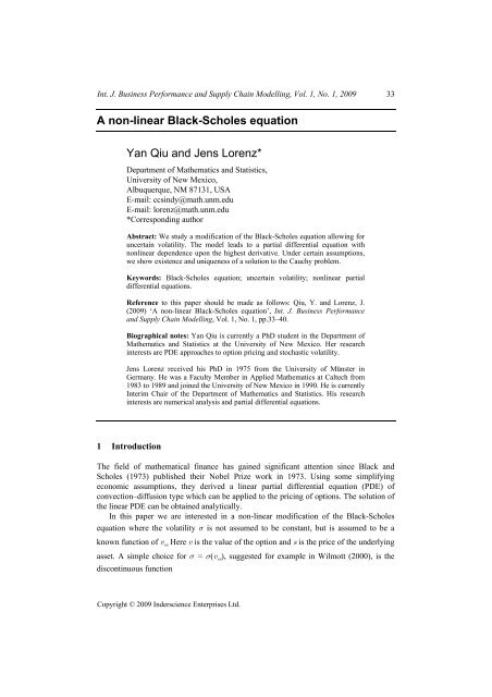
38 Y. Qiu and J. LorenzThe function σ d in (4) is not smooth, of course, but we can approximate σ d by asmooth function like1 + − 1 + − ⎛ ⎞= + − − tanh 1σ σ σ σ σ ⎜ uεxx ⎟2 2,⎝ε⎠( uxx) ( ) ( )ε >0Figure 1The graphs of σ d (left) and σ ε (right) for σ + = 0.3, σ – = 0.2 and ε = 0.3 (see onlineversion for colours)σ (u )σ d xx ε(u xx)0.30.3σ d0.25σ ε0.250.20.20.15−10 −5 0 5 10u xx0.15−10 −5 0 5 10u xxDifferentiate equation (6) twice with respect to x and set w = u xx to obtain= ( ) + ′( )where ( ) ( ) ′( )w h w w h w w 2 (7)t xx xh w = G w + G w w . It will be convenient to consider the slightly moregeneral equation( ) ( ) ( ) ( )w = h w w + g w, w , w x, 0 = f x ,(8)t xx xwhere h(w), g(w, w x ) and f(x) are C ∞ functions of their arguments. To concentrate on theessential mathematical difficulty, the non-linear volatility coefficient, we assume theinitial function f(x) to be 1-periodic; we then seek a solution w(x, t), of (8) which is1-periodic in x. Other boundary conditions will be considered in future work.Theorem 4.1Consider the 1-periodic initial value problem (8) under the aboveassumptions. In addition, assume that h(w) ≥ k > 0 for all real w andthat h and g and all their derivatives are bounded functions. Then thereis a unique C ∞ solution w(x, t) which is 1-periodic in x. The solutionsexists for 0 ≤ t < ∞.

A non-linear Black-Scholes equation 39Remark: If h or g or their derivatives are unbounded, one can use a cut-off argument andreplace h or g by functions h % or %g which satisfy the conditions of the theorem. For theoriginal problem, one then obtains a result which is local in time.To prove the existence part of the theorem, we define a sequence of functions w n (x, t)via the iteration( ) ( ) ( ) ( )n+ 1 n n+ 1 n n n+1t xx xw = h w w + g w , w , w x, 0 = f x , n = 0,1,2, K (9)starting with w 0 (x, t) ≡ f(x). Since the problem (9) is linear parabolic, there is nodifficulty in establishing existence, uniqueness and smoothness of the functionsw n (x, t) ≡ w n (x + 1, t) for 0 ≤ t < ∞.It can then be shown and this is the main mathematical difficulty, that the functionsw n (x, t) are ‘uniformly’ smooth in any finite time interval. More precisely, for any fixed0 < T < ∞, all derivatives are bounded independently of the iteration index n:p+q∂ nsup max max w x, t C p, q,Tx t T p qn 0≤ ≤ ∂x∂t( ) ≤ ( )

40 Y. Qiu and J. Lorenz3 The case of a non-smooth volatility σ d (μ xx ) can also be treated as a free boundaryvalue problem where lines (x(t), t) with μ xx (x(t), t) = 0 will be determined as freeboundaries.ReferencesBlack, F. and Scholes, M. (1973) ‘The pricing of options and corporate liabilities’, J. PoliticalEconomics, Vol. 81, pp.637–654.Kreiss, H-O. and Lorenz, J. (1989) Initial-boundary Value Problems and the Navier-stokesEquations, Academic Press, Boston.Wilmott, P. (2000) Paul Wilmott on Quantitative Finance Volume One and Volume Two,John Wiley & Sons Ltd, Chichester.