Translation Exposure and Firm Value, Evidence From Australian ...

More documents

Recommendations

Info

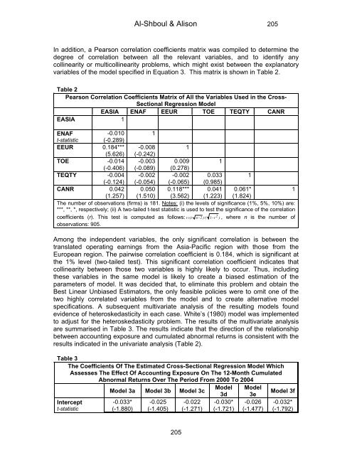
Al-Shboul & Alison 205In addition, a Pearson correlation coefficients matrix was compiled to determine thedegree of correlation between all the relevant variables, and to identify anycollinearity or multicollinearity problems, which might exist between the explanatoryvariables of the model specified in Equation 3. This matrix is shown in Table 2.Table 2Pearson Correlation Coefficients Matrix of All the Variables Used in the Cross-Sectional Regression ModelEASIA ENAF EEUR TOE TEQTY CANREASIA 1ENAF-0.010 1t-statistic (-0.289)EEUR 0.184*** -0.0081(5.626) (-0.242)TOE -0.014 -0.003 0.009 1(-0.406) (-0.089) (0.278)TEQTY -0.004 -0.002 -0.002 0.033 1(-0.124) (-0.054) (-0.065) (0.985)CANR 0.042 0.050 0.118*** 0.041 0.061*1(1.257) (1.510) (3.562) (1.223) (1.824)The number of observations (firms) is 181. Notes: (i) the levels of significance (1%, 5%, 10%) are:***, **, *, respectively; (ii) A two-tailed t-test statistic is used to test the significance of the correlationcoefficients (r). This test is computed as follows: t= (r n−2 )/( 1−r2) , where n is the number ofobservations: 905.Among the independent variables, the only significant correlation is between thetranslated operating earnings from the Asia-Pacific region with those from theEuropean region. The pairwise correlation coefficient is 0.184, which is significant atthe 1% level (two-tailed test). This significant correlation coefficient indicates thatcollinearity between those two variables is highly likely to occur. Thus, includingthese variables in the same model is likely to create a biased estimation of theparameters of model. It was decided that, to eliminate this problem and obtain theBest Linear Unbiased Estimators, the only feasible policies were to omit one of thetwo highly correlated variables from the model and to create alternative modelspecifications. A subsequent multivariate analysis of the resulting models foundevidence of heteroskedasticity in each case. White’s (1980) model was implementedto adjust for the heteroskedasticity problem. The results of the multivariate analysisare summarised in Table 3. The results indicate that the direction of the relationshipbetween accounting exposure and cumulated abnormal returns is consistent with theresults indicated in the univariate analysis (Table 2).Table 3The Coefficients Of The Estimated Cross-Sectional Regression Model WhichAssesses The Effect Of Accounting Exposure On The 12-Month CumulatedAbnormal Returns Over The Period From 2000 To 2004Model ModelModel 3a Model 3b Model 3cModel 3f3d 3eInterceptt-statistic-0.033*(-1.880)-0.025(-1.405)-0.022(-1.271)-0.030*(-1.721)-0.026(-1.477)-0.032*(-1.792)205
Al-Shboul & Alison 206EASIA0.035 0.068*0.069*(0.938) (1.944)(1.970)ENAF0.001***0.001***0.001*** 0.001***(3.483)(3.418)3.423 3.483EEUR0.328***0.338***0.339***(2.792)(2.984)(2.995)TEARNS0.024* 0.024* 0.024* 0.023* 0.024* 0.023*(1.812) (1.858) (1.855) (1.803) (1.862) (1.807)TEQTY0.078* 0.077* 0.077* 0.077* 0.077* 0.078*(1.711) (1.732) (1.741) (1.712) (1.733) (1.713)Observations 905 905 905 905 905 905Adjusted R 2 4% 3% 4% 3% 3% 4%F-statisticsp-value4.0550.0012.1120.0975.8080.0012.3260.0732.1670.0714.9630.001Notes: (i) t-statistic is used with the levels of significance (1%, 5%, 10%) are: ***, **, *, respectively;(ii) CANR it = β 0 + β 1 EASIA it + β 2 EEUR it + β 3 ENAF it + β 4 TOF it + β 5 TEQTY it + η it ; where: CANR it , isthe average of the cumulated monthly abnormal returns, over each calendar year for the estimationperiod 2000 – 2004, for each firm i; EASIA it , the annual Asian translated operating earningsdivided by the total operating earnings for firm i over 2000-2004; EEUR it , the annual Europeantranslated operating earnings divided by the total operating earnings for firm i; ENAF it , the annualNAFTA translated operating earnings divided by the total operating earnings for firm i; TOE it , is theannual total operating earnings divided by total sales for firm i. TEQTY it , is the total annualtranslated profit (loss) on assets and liabilities against shareholders’ equity scaled to the totalshareholders’ equity for firm i; β 0 – β 5 , are the regression coefficients; η it , is the error term. All theobservations of the independent variables are collected over each financial year for the period 2000– 2004 (905 observations). An OLS is used to estimate the parameters of the model with White’s(1980) model to adjust for heteroskedasticity.The results in Table 3 clearly indicate that all the variables used in models (3a – 3f)are found to be significantly positively associated with cumulative abnormal returns.This suggests that the variables, annual translated operating earnings, annualtranslated operating earnings from each region, and the translated gain or losscharged annually against shareholders’ equity, which serve as proxies for translationexposure, are all viewed by the market as value additive. Positive translationadjustments are associated with increases in market value. This result is consistentwith the findings of Martin et al. (1998), but at variance with the findings of severalother studies (e.g. Callaghan & Bazaz, 1992; Soo & Soo, 1994; Pourciau & Schaefer,1995; Bartov, 1997; Dhaliwal et al., 1999).The full model 3(a) provides estimates of the relevant coefficients, without taking intoaccount the collinearity problem between the translated earnings from Asia andEurope. It was found that, total translated operating earnings, translated operatingearnings from three regions, and gains or losses on assets and liabilities charged toshareholders’ equity are all related to accounting exposure. These relationships areall significant with the exception of the relationship between accounting exposure andthe translated operating earnings from Asia. It was considered that this inconsistencyin the results may have been due to the collinearity problem identified earlier, andthree alternative models, 3(b), 3(c) and 3(d) were implemented accordingly. Theresults indicate a significant relationship between all the relevant estimatedcoefficients of these three models, and accounting exposure. Again, to deal with thecollinearity problem, the final two alternative models to 3(a), i.e. models 3(e) and 3(f),which omit the translated operating earnings from the European and Asia-Pacific206
Page 2 and 3: Al-Shboul & Alison 193Firstly, the
Page 6 and 7: Al-Shboul & Alison 197group reporti
Page 8 and 9: Al-Shboul & Alison 199to SFAS No. 5
Page 10 and 11: Al-Shboul & Alison 201four-factor r
Page 12 and 13: Al-Shboul & Alison 203firstly used
Page 16 and 17: Al-Shboul & Alison 207regions, resp
Page 18 and 19: Al-Shboul & Alison 209Cornell, B. 1
Page 20 and 21: Al-Shboul & Alison 211O'Brien, T. 1

Translation Exposure and Firm Value, Evidence From Australian ...

You also want an ePaper? Increase the reach of your titles

Delete template?

Save as template?