Appendix 4-2-D CALPUFF and CALMET Methods and Assumptions

Taseko Prosperity Gold-Copper Project 

Appendix 4-2-D: CALPUFF and CALMET Methods and Assumptions 

Appendix 4-2-D CALPUFF and CALMET Methods and 

Assumptions 

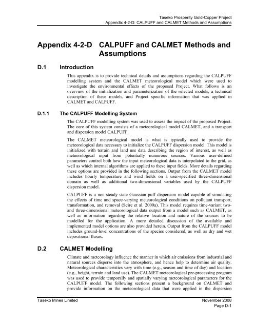
D.1 Introduction 

This appendix is to provide technical details and assumptions regarding the CALPUFF 

modelling system and the CALMET meteorological model which were used to 

investigate the environmental effects of the proposed Project. What follows is an 

overview of the initialization and parameterization of the selected models, a technical 

description of these models, and Project specific information that was applied in 

CALMET and CALPUFF. 

D.1.1 The CALPUFF Modelling System 

The CALPUFF modelling system was used to assess the impact of the proposed Project. 

The core of this system consists of a meteorological model CALMET, and a transport 

and dispersion model CALPUFF. 

The CALMET meteorological model is what is typically used to provide the 

meteorological data necessary to initialize the CALPUFF dispersion model. This model is 

initialized with terrain and land use data describing the region of interest, as well as 

meteorological input from potentially numerous sources. Various user-defined 

parameters control both how the input meteorological data is interpolated to the grid, as 

well as which internal algorithms are applied to these input fields. More details regarding 

these options are provided in the following sections. Output from the CALMET model 

includes hourly temperature and wind fields on a user-specified three-dimensional 

domain as well as additional two-dimensional variables used by the CALPUFF 

dispersion model. 

CALPUFF is a non-steady-state Gaussian puff dispersion model capable of simulating 

the effects of time and space-varying meteorological conditions on pollutant transport, 

transformation, and removal (Scire et al. 2000a). This model requires time-variant twoand 

three-dimensional meteorological data output from a model such as CALMET, as 

well as information regarding the relative location and nature of the sources to be 

modelled for the application. A more detailed discussion of the available and 

implemented model options are also provided herein. Output from the CALPUFF model 

includes ground-level concentrations of the species considered, as well as dry and wet 

depositional fluxes. 

D.2 CALMET Modelling 

Climate and meteorology influence the manner in which air emissions from industrial and 

natural sources disperse into the atmosphere, and hence help to determine air quality. 

Meteorological characteristics vary with time (e.g., season and time of day) and location 

(e.g., height, terrain and land use). The CALMET meteorological pre-processing program 

was used to provide temporally and spatially varying meteorological parameters for the 

CALPUFF model. The following sections present a background on CALMET and 

provide information on the meteorological data that were applied in the dispersion 

Taseko Mines Limited November 2008 

Page D-1



modelling assessment of the Project. Results of the analysis performed on the 

meteorological dataset are also provided. 

D.2.1 Model Description 

SOURCE: Scire et al. 2000b 

The following description of the CALMET model’s major model algorithms and options 

are all excerpts from the CALMET model’s user manual (Scire et al. 2000b). 

The CALMET meteorological model consists of a diagnostic wind field module and 

micrometeorological modules for overwater and overland boundary layers. The 

diagnostic wind field module uses a two-step approach to the computation of the wind 

fields (Douglas and Kessler 1988), as illustrated in Figure D-1. 

Figure D–1 Flow Diagram of Diagnostic Wind Module in CALMET 


Page D-2



In the first step, an initial guess wind field is adjusted for kinematic effects of terrain, 

slope flows, and terrain blocking effects to produce a Step 1 wind field. The initial guess 

field is either a uniform field based on available observational data or the output from the 

NCAR/PSU Mesoscale Modelling System (MM4/MM5). The second step consists of an 

objective analysis procedure to introduce observational data into the Step 1 wind field to 

produce a final wind field. An option is provided to allow gridded prognostic wind fields 

to be used by CALMET, which may better represent regional flows and certain aspects of 

sea breeze circulations and slope/valley circulations. Wind fields generated by the 

prognostic wind field module can be input to CALMET as either the initial guess field or 

the Step 1 wind field. 

D.2.2 Diagnostic Wind Field Module – Initial Guess Field 

Options exist within CALMET to create an initial guess field either by interpolating 

observation data or by using output from a prognostic meteorological model, such as the 

NCAR/PSU Mesoscale Modelling System (MM4/MM5). The prognostic model data is 

usually run over a very large domain with much coarser resolution than that applied with 

CALMET. CALMET will interpolate the prognostic data to develop a 3-D fine scale first 

guess field of wind speeds and directions. 

D.2.2.1 Step 1 Wind Field 

The step one wind field is adjusted for kinematic effects of terrain, slope flows, and 

blocking effects as follows: 

• Kinematic Effects of Terrain: The approach of Liu and Yocke (1980) is used to 

evaluate kinematic terrain effects. The domain scale winds are used to compute a 

terrain forced vertical velocity, subject to an exponential, stability dependent decay 

function. The kinematic effects of terrain on the horizontal wind components are 

evaluated by applying a divergence minimisation scheme to the initial guess wind 

field. The divergence minimisation scheme is applied iteratively until the three 

dimensional divergence is less than a threshold value. 

• Slope Flows: An empirical scheme based on Allwine and Whiteman (1985) is used to 

estimate the magnitude of slope flows in complex terrain. The slope flow is 

parameterised in terms of the terrain slope, terrain height, domain scale lapse rate, 

and time of day. The slope flow wind components are added to the wind field 

adjusted for kinematic effects. 

• Blocking Effects: The thermodynamic blocking effects of terrain on the wind flow are 

parameterised in terms of the local Froude number (Allwine and Whiteman 1985). If 

the Froude number at a particular grid point is less than a critical value and the wind 

has an uphill component, the wind direction is adjusted to be tangent to the terrain. 

D.2.2.2 Step 2 Wind Field 

The wind field resulting from the adjustments of the initial guess wind described above is 

the Step 1 wind field. The second step of the procedure involves the introduction of 

observational data into the Step 1 wind field through an objective analysis procedure. An 

inverse distance squared interpolation scheme is used which weighs observational data 

heavily in the vicinity of the observational station, while the Step 1 wind field dominates 

the interpolated wind field in regions with no observational data. The resulting wind field 


Page D-3



is subject to smoothing, an optional adjustment of vertical velocities based on the O'Brien 

(1970) method, and divergence minimisation to produce a final Step 2 wind field. 

D.2.2.3 Micrometeorology Modules 

The CALMET model contains two boundary layer models for application to overland and 

overwater grid cells: 

• Overland Boundary Layer Model: Over land surfaces, the energy balance method of 

Holtslag and van Ulden (1983) is used to compute hourly gridded fields of the 

sensible heat flux, surface friction velocity, Monin Obukhov length, and convective 

velocity scale. Mixing heights are determined from the computed hourly surface heat 

fluxes and observed temperature soundings using a modified Carson (1973) method 

based on Maul (1980). The model also determines gridded fields of PGT stability 

class and optional hourly precipitation rates. 

• Overwater Boundary Layer Model: The aerodynamic and thermal properties of water 

surfaces suggest that a different method is best suited for calculating the boundary 

layer parameters in the marine environment. A profile technique (Garratt 1977; 

Hanna et al. 1985), using air sea temperature differences, is used in CALMET to 

compute the micrometeorological parameters in the marine boundary layer. 

D.2.3 CALMET Modelling Domain 

The CALMET modelling domain area adopted for this assessment extends 30 km out 

from the Project site for a 60 by 60 km area, as shown in Figure D-2. A horizontal grid 

spacing of 500 m was selected for the CALMET simulation; the study area therefore 

corresponds to 120 rows by 120 columns. With this grid spacing, it was possible to 

maximize run time and file size efficiencies while still capturing large-scale terrain 

feature influences on wind flow patterns. 

To properly simulate pollution transport and dispersion, it is also important to simulate 

the typical vertical profiles of wind direction, wind speed, temperature, and turbulence 

intensity within the atmospheric boundary layer (i.e., the layer within about 2000 metres 

above the Earth’s surface). To capture this vertical structure, ten vertical layers were 

selected for the extent of the modelling domain area. CALMET defines a vertical layer as 

the midpoint between two faces (i.e., 11 faces corresponds to 10 layers, with the lowest 

layer always being ground level or 10 m). The vertical faces used in this study are: 0, 20, 

40, 80, 160, 320, 640, 1000, 1500, 2200 and 3000 m. 

D.2.4 CALMET Modelling Period 

The CALMET meteorological model was run for one full year from January 1, 2002 to 

December 31, 2002. This year was chosen for assessment so that an available 12 km 

MM5 (a mesoscale meteorological model assimilation produced by Penn State/NCAR) 

prognostic dataset from Environment Canada could be input into CALMET. Two 

separate simulations were run to account for the different land use characteristics due to 

snow and ice during the winter months. For the purposes of dispersion modelling, winter 

was defined to span from December to February. 

The meteorological data produced by the MM5 model were used as an initial guess field 

(Scire et al. 2000b). The CALMET model adjusted the initial guess field for the 


Page D-4

D.2.5 Model Options 



kinematic effects of terrain, slope flows, and terrain blocking effects using the finer 

scaled CALMET terrain data to produce a modified wind field. 

Table D-1 provides a detailed summary of all CALMET model user options selected for 

the modelling done in this assessment. Model default values, as recommended by the 

United States Environmental Protection Agency (U.S. EPA 1998), are presented for 

comparative purposes. In most cases, these default values were used. 


Page D-5



Figure D–2 CALMET Domain and Location of Extraction Point 


Page D-6

Table D–1 CALMET Model User Options 



Input Group Parameter 

U.S. EPA 

Default 

Value Used Selection Description 

Group 1: General IBYR - 2002 Starting year 

Run Control IBMO - 1 Starting month 

Parameters IBDY - 1 Starting day 

IBHR - 0 Starting hour 

IBSEC - 0 Starting second 

IEYR - 2003 Ending year 

IEMO - 1 Ending month 

IEDY - 1 Ending day 

IEHR - 0 Ending hour 

IBSEC - 0 Ending second 

ABTZ - 8 Time zone 

NSECDT - 3600 Model Time Step (seconds) 

IRTYPE 1 1 Run type 

LCALGRD T T Special data fields are computer 

ITEST 2 2 Flag to not stop run after setup phase 

Group 2: Map PMAP UTM UTM Map Projection is UTM 

Projection and FEAST 0.0 0.0 False Easting (Not Used) 

Grid Control FNORTH 0.0 0.0 False Northing (Not Used) 

Parameters IUTMZN - 9 UTM Zone 

UTMHEM N N Northern Hemisphere for UTM Projection 

RLAT0 - 0N Latitude of Projection Origin (Not Used) 

RLON0 - 0E Longitude of Projection Origin (Not Used) 

XLAT1 - 0N Latitude of 1 st Parallel (Not Used) 

XLAT2 - 0N Latitude of 2 nd Parallel (Not Used) 

DATUM WGS-84 NAR-C NORTH AMERICAN 1983 GRS 80 Spheroid, MEAN FOR 

CONUS (NAD83) 

NX - 120 Number of X grid cells 

NY - 120 Number of Y grid cells 

DGRIDKM - 0.5 Grid spacing in X and Y directions (km) 

XORIGKM - 427.29 Reference Easting of SW corner of SW grid cell in UTM (km) 

YORIGKM - 5671.03 Reference Northing of SW corner of SW grid cell in UTM (km) 

NZ - 10 Number of vertical grid cells 

ZFACE - 0, 20, 40, 80, 160, 

320, 640, 1000, 1500, 

2200, 3000 

Vertical cell face heights of the NZ vertical layers (m) 


Page D-7

Table D–1 CALMET Model User Options (cont’d) 




U.S. EPA 

Default 


Group 3: Output LSAVE T T Save met data in unformatted output files 

Options 

IFORMO 1 1 Type of unformatted output file 

LPRINT F T Print meteorological fields 

IPRINF 1 12 Print interval in hours 

IUVOUT 0 0 Do not print u, v wind components 

IWOUT 0 0 Do not print w wind component 

ITOUT 0 0 Do not print 3-D temperature fields 

Specify Meteorological Fields to Print 

STABILITY 1 Print PGT stability class 

USTAR 0 Do not print friction velocity 

MONIN 0 Do not print Monin-Obukhov length 

MIXHT 1 Print mixing height 

WSTAR 0 Do not print convective velocity scale 

PRECIP 1 Do not print precipitation rate 

SENSHEAT 0 Do not print sensible heat flux 

CONVZI 0 Do not print convective mixing height 

Testing and Debugging Options 

LDB F F Print input and internal variables 

NN1 1 1 First time step to print data 

NN2 1 1 Last time step to print data 

LDBCST F F Do not print distance to land internal variables 

IOUTD 0 0 Control variable to note write test data to disk 

NZPRN2 1 0 Number of levels to print 

IPR0 0 0 Do not print interpolated wind components 

IPR1 0 0 Do not print the terrain adjusted wind components 

IPR2 0 0 Do not print smoothed wind components and initial divergence 

fields 

IPR3 0 0 Do not print final wind speed and direction 

IPR4 0 0 Do not print final divergence fields 

IPR5 0 0 Do not print winds after kinematic effects are added 

IPR6 0 0 Do not print winds after the Froude number adjustment 

IPR7 0 0 Do not print wind after slope flow adjustment 

IPR8 0 0 Do not print final wind field components 


Page D-8





U.S. EPA 

Default 


Group 4: 

NOOBS 0 2 No surface, overwater, or upper air observations 

Meteorological 

Use MM4/MM5/3D for surface, overwater, and upper air data 

Data Options NSSTA - 0 Number of surface stations 

Group 5: Wind 

Field Options and 

Parameters 

NPSTA - -1 Number of precipitation stations 

ICLOUD 0 3 Gridded cloud cover computed from prognostic fields 

IFORMS 2 2 Surface meteorological data file format 

IFORMP 2 2 Precipitation data file format 

IFORMC 2 2 Cloud data file format 

IWFCOD 1 1 Wind field diagnostic model selected 

IFRADJ 1 1 Use Froude number adjustment 

IKENE 0 0 Do not use Kinematic effects adjustment 

IOBR 0 1 Use O’Brien procedure to adjust vertical velocity 

ISLOPE 1 1 Compute slope flow effects 

IEXTRP -4 1 No extrapolation is done 

ICALM 0 0 Do not extrapolate surface winds if calm 

BIAS 8*0 8*0 Layer dependent bias in vertical interpolation between surface and 

upper air data in first guess field. Prognostic data is used, therefore the 

model ignores this option. 

RMIN2 -1 -1 Minimum distance from nearest upper air station to surface station for 

which extrapolation of surface winds at surface station be allowed. Not 

Used if NOOBS=1 

IPROG 0 14 Use gridded prognostic wind field model output as input to the diagnostic 

wind field model 

ISTEPPG 1 1 Time step (hours) of input prognostic data 

IGFMET 0 0 Use coarse CALMET fields as initial guess fields 

LVARY F F Use varying radius of influence. if no stations are found within 

RMAX1,RMAX2, or RMAX3, then the closest station will be used. 

RMAX1 - 30 Maximum radius of influence over land in the surface layer (km) 

RMAX2 - 30 Maximum radius of influence over land aloft (km) 

RMAX3 - 60 Maximum radius of influence over water (km) 

RMIN 0.1 0.1 Minimum radius of influence used in the wind field interpolation (km) 

TERRAD 15 3.5 Radius of influence of terrain features (km) 

R1 - 3 Relative weighting of the first guess field and observations in the surface 

layer (km) 


Page D-9





U.S. EPA 

Default 


Group 5: Wind R2 - 6 Relative weighting of the first guess field and observations in the 

Field Options and 

upper layer (km) 

Parameters RPROG - 0 Relative weighting of the prognostic wind field data (km) (Not 

(Cont…) 

Used) 

DIVLIM 5 E-6 5 E-6 Maximum acceptable divergence in divergence minimization 

procedure 

NITER 50 50 Maximum number of iterations in the divergence minimization 

procedure 

NITER2 99*8 99*8 Maximum number of stations used in each layer for the 

interpolation of data to a grid point 

NSMTH 2, 

2 , 7 , 7 , 14 , 14 , 28 , Number of passes in the smoothing procedure 

(nz - 1)*4 28 , 28 

CRITFN 1 1 Critical Froude number 

ALPHA 1 0.1 Empirical factor controlling Kinematic effects 

FEXTR2 0*8 0*8 Multiplicative scaling factor for extrapolation of surface 

observations to upper layers (Not Used) 

NBAR 0 0 Number of barriers to interpolation of wind 

KBAR NZ 12 Level (1 to NZ) up to which barriers apply 

XBBAR - 0 X coordinate of beginning of barrier (Not Used) 

YBBAR - 0 Y coordinate of beginning of barrier (Not Used) 

XEBAR - 0 X coordinate of end of barrier (Not Used) 

YEBAR - 0 Y coordinate of end of barrier (Not Used) 

IDIOPT1 0 0 Computer surface temperature internally from surface monitoring 

data for Diagnostic Wind Module 

ISURFT - 3 Surface meteorological station to use for the surface temperature 

in Diagnostic Wind Module 

IDIOPT2 0 0 Domain-averaged temperature lapse rate computed internally 

from upper air soundings 

IUPT - 0 Upper air station to use for the domain-scale lapse rate (not 

used). 

ZUPT 200 200 Depth through which the domain-scale lapse rate is computer (m) 

IDIOPT3 0 0 Domain-averaged wind components calculated internally 

IUPWND -1 -1 Upper air station to use for the domain scale winds 

ZUPWND 1, 1000 1, 2500 Bottom and top of layer through which domain-scale winds are 

computed (m) 


Page D-10





U.S. EPA 

Default 


Group 5: Wind IDIOPT4 0 0 Observed surface wind components read from surface data file 

Field Options and IDIOPT5 0 0 Observed upper wind components read from upper air data file 

Parameters LLBREZE F F Do not use lake breeze module 

(Cont…) 

NBOX - 0 Number of lake breeze regions 

XG1 - 0 X grid line 1 of region of interest 

XG2 - 0 X grid line 2 of region of interest 

YG1 - 0 Y grid line 1 of region of interest 

YG2 - 0 Y grid line 2 of region of interest 

XBCST - 0 X point defining coast line 

YBCST - 0 Y point defining coast line 

XECST - 0 X point defining coast line 

YECST - 0 Y point defining coast line 

NLB - 0 Number of station in the region 

METBXID - 0 Station’s ID in the region 

Group 6: Mixing CONSTB 1.41 1.41 Empirical mixing height equation constant, neutral conditions 

Height, 

CONSTE 0.15 0.15 Empirical mixing height equation constant, convective conditions 

Temperature and CONSTN 2400 2400 Empirical mixing height equation constant, stable conditions 

Precipitation CONSTW 0.16 0.16 Empirical mixing height equation constant, over water conditions 

FCORIO 1.0E-4 1.2E-4 Coriolis Parameters, adjusted for latitude 

IAVEZI 1 1 Use spatial averaging of mixing heights 

MNMDAV 1 1 Maximum search radius (grid cells) 

HAFANG 30 30 Half-angle upwind looking cone for averaging 

ILEVZI 1 1 Layer of winds used in upwind averaging 

IMIXH 1 1 Use the Maul-Carson method for land and water cells to compute 

convective mixing height 

THRESHL 0.05 0.05 Threshold buoyancy flux to sustain convective mixing height 

growth overland (W/m 2 ) 

THRESHW 0.05 0.05 Threshold buoyancy flux to sustain convective mixing height 

growth overwater (W/m 2 ) 

ITWPROG 0 0 Use SEA.DAT to determine overwater lapse rates and deltaT (or 

assume neutral conditions if missing) 

ILUOC3D 16 16 Land Use category for ocean in 3D.DAT datasets 

DPTMIN 0.001 0.001 Minimum potential temperature lapse rate in the stable layer 

above the current convective mixing height (K/m) 


Page D-11





U.S. EPA 

Default 


Group 6: Mixing DZZI 200 200 Depth of layer above current convective mixing height through 

Height, 

which lapse rate is computed (m) 

Temperature and ZIMIN 50 50 Minimum overland mixing height (m) 

Precipitation ZIMAX 3000 3000 Maximum overland mixing height (m) 

(Cont…) 

ZIMINW 50 50 Minimum over water mixing height (m) 

ZIMAXW 3000 3000 Maximum over water mixing height (m) 

ICOARE 10 10 COARE Method with no wave parameterization used to 

determine overwater surface flux 

DSHELF 0 0 Coastal/Shallow water length scale (km) 

IWARM 0 0 COARE warm layer computation turned off 

ICOOL 0 0 COARE cool skin layer computation turned off 

IRHPROG 0 1 Use prognostic RH 

ITPROG 0 2 No surface or upper air observations 

Use MM5/3D for surface and upper air data 

IRAD 1 1 Use 1/R interpolation scheme 

TRADKM 500 500 Radius of influence for temperature interpolation (km) 

NUMTS 5 2 Maximum number of stations to include in interpolation 

IAVET 1 1 Use spatial averaging of temperature data 

TGDEFB -0.0098 -0.0098 Default temperature gradient below the mixing height, over water 

(K/m) 

TGDEFA -0.0045 -0.0045 Default temperature gradient above the mixing height, over water 

(K/m) 

JWAT1 - 999 Beginning land use category for temperature interpolation over 

water. Make bigger than largest land use to disable. 

JWAT2 - 999 Ending land use category for temperature interpolation over 

water. Make bigger than largest land use to disable. 

NFLAGP 2 2 Use 1/R 2 interpolation scheme for precipitation interpolation 

SIGMAP 100 100 Radius of influence for interpolation from precipitation stations 

(km) 

CUTP 0.01 0.01 Minimum precipitation rate cut off (mm/hr) 


Page D-12




Input Group Parameter U.S. EPA Default Value Used Selection Description 

Group 7: Surface 

meteorological station 

parameters 

No Surface Meteorological Stations Used 

Group 8: Upper Air 

Meteorological Station 

Parameters 

No Upper Air Radiosonde Stations Used 

Group 9: Upper Air 

Meteorological Station 

Parameters 

No Precipitation Stations Used 


Page D-13

D.2.6 Meteorological Data Summary 



The local meteorology of the region must be characterized to evaluate the short-term 

atmospheric dispersion and transport of air emissions. The data required to predict 

dispersion and transport include the following main components: 

• wind speed and direction 

• ambient air temperature 

• mixing layer depth 

• atmospheric stability 

Meteorological conditions for the Project area were extracted from CALMET output for a 

location in the vicinity of the Project mine pit (see Figure D-2). 

D.2.6.1 Winds 

Wind roses are an efficient and convenient means of presenting wind data. The length of 

the radial barbs gives the total percent frequency of winds from the indicated direction, 

while portions of the barbs of different widths indicate the frequency associated with 

each wind speed category. Figure D–3 presents a wind rose for wind data applied in 

dispersion modelling. Observed winds commonly blow from the southeast, southwest and 

northwest. Figure D–4 presents frequency distributions for various wind speed classes. 

Approximately 63.5 percent of wind speeds were below 3.6 m/s (13 km/h). 

Figure D–5 presents seasonal wind roses for meteorological data applied in dispersion 

modelling. Maximum wind speeds for spring and summer were 18 and 10.7 m/s (65 and 

39 km/h), respectively. Maximum wind speeds for fall and winter were 16.2 and 22.1 m/s 

(58 and 80 km/h), respectively. Average seasonal wind speeds ranged from 2.3 to 5.2 m/s 

(8 to 19 km/h). 


Page D-14



NORTH 

3% 

WEST EA ST 

SOUTH 


Page D-15 

6% 

9% 

12% 

15% 

WIND SPEED 

(m/s) 

>= 11.1 

8.8 - 11.1 

5.7 - 8.8 

3.6 - 5.7 

2.1 - 3.6 

1.0 - 2.1 

Calms: 16.40% 

Figure D–3 Wind Roses Depicting Hourly Surface Winds for Meteorological 

Data Applied in Dispersion Modelling (2002) 

30 

25 

20 

% 

15 

10 

5 

0 

16.4 

19.6 

27.5 

19.6 

y 

11.7 

2.7 2.6 

Calms 1.0 - 2.1 2.1 - 3.6 3.6 - 5.7 5.7 - 8.8 8.8 - 11.1 >= 11.1 

Wind Class (m/s) 

Figure D–4 Wind Class Frequency Distribution for Meteorological Data 

Applied in Dispersion Modelling (2002)



Spring Summer 

NORTH 

3% 

WEST EA ST 

SOUTH 

NORTH 

SOUTH 

6% 

9% 

12% 

15% 

3% 

WEST EA ST 

WIND SPEED 

(m/s) 

>= 11.1 

8.8 - 11.1 

5.7 - 8.8 

3.6 - 5.7 

2.1 - 3.6 

1.0 - 2.1 

Calms: 16.35% 


Page D-16 

NORTH 

3% 

WEST EA ST 

SOUTH 

Fall Winter 

6% 

9% 

12% 

15% 

WIND SPEED 

(m/s) 

>= 11.1 

8.8 - 11.1 

5.7 - 8.8 

3.6 - 5.7 

2.1 - 3.6 

1.0 - 2.1 

Calms: 15.20% 

NORTH 

SOUTH 

6% 

9% 

12% 

15% 

4% 

WEST EA ST 

8% 

12% 

16% 

20% 

WIND SPEED 

(m/s) 

>= 11.1 

8.8 - 11.1 

5.7 - 8.8 

3.6 - 5.7 

2.1 - 3.6 

1.0 - 2.1 

Calms: 28.31% 

WIND SPEED 

(m/s) 

>= 11.1 

8.8 - 11.1 

5.7 - 8.8 

3.6 - 5.7 

2.1 - 3.6 

1.0 - 2.1 

Calms: 5.51% 

Figure D–5 Seasonal Wind Rose for Meteorological Data Applied in Dispersion 

Modelling (2002)



D.2.6.2 Ambient Air Temperature 

Seasonal frequency distributions of hourly surface ambient air temperature for 

meteorological data applied in dispersion modelling are shown in Figure D–6. Median 

ambient air temperatures for spring, summer, autumn, and winter were -2.4, 10.5, 2.4, 

and -5.5°C, respectively. Extreme minimum and maximum temperatures for the period 

were equal to -33.6 and 25.4°C, respectively. 

D.2.6.3 Mixing Height 

The mixing layer height is a parameter used to define the effective depth of the 

atmosphere through which dispersion of pollutants can take place. Heat transfer to the 

atmosphere at the earth’s surface results in convective (vertical) mixing and consequently 

changes the vertical temperature profile, which defines the atmospheric lapse rate. 

The depth of the mixed layer is dependent on thermal effects (e.g., vertical temperature 

stratification) and mechanical effects caused by topography, surface roughness, and wind 

speed. The height of the mixing layer determines the vertical extent to which emissions 

are able to diffuse. Seasonal frequency distributions of mixing heights are shown in 

Figure D–7. 

D.2.6.4 Atmospheric Stability 

Atmospheric turbulence near the earth’s surface is often described in terms of 

atmospheric stability, which is governed by both thermal and mechanical factors. 

Atmospheric stability can, very broadly, be classified as stable, neutral, or unstable. 

Stable atmospheric conditions occur when vertical motion in the atmosphere is 

suppressed. With respect to air quality, this means pollutants emitted near ground-level 

are not well-dispersed and have a larger effect on local ambient levels. This type of 

situation frequently occurs at night, when the earth’s surface emits thermal radiation and 

cools. Air in contact with the ground thus becomes cooler and denser than the air aloft. 

This phenomenon is referred to as a ground-based temperature inversion and is often 

associated with poor air quality conditions. 

Unstable atmospheric conditions are also highly dependent on radiation at the earth’s 

surface, and most frequently occur during day-time hours. During such times, as shortwave 

energy from the sun heats the ground, air in contact with the ground becomes 

warmer and less dense than the air aloft. Subsequently, vertical motion in the atmosphere 

is enhanced and the atmosphere is said to be unstable. 

When a balance exists between incoming and outgoing radiation, there is no net heating 

or cooling of the air in contact with the ground and vertical motions of the atmosphere are 

neither enhanced nor suppressed. Such an atmosphere is described as neutral and exists 

during overcast skies or during transition from unstable to stable conditions. 

Atmospheric stability was characterized using the Pasquill (1961) method based on wind 

data and cloud cover. Figure D-8 presents an overall stability frequency distribution. 

Seasonal stability frequencies are summarized in Table D–2. Unstable conditions 

(Categories A, B, C) occurred most often during the spring and summer months while 

stable conditions (Categories E and F) occurred most often during autumn months. 

Neutral conditions (Category D) were most frequent in winter months, a reflection of the 

higher wind speeds that also occurred during the winter. 


Page D-17



Figure D–6 Seasonal Cumulative Frequency Distributions of Hourly 

Average Temperature for Meteorological Data Applied in 

Dispersion Modelling 

Figure D–7 Seasonal Cumulative Frequency Distributions of Hourly 

Average Mixing Height for Meteorological Data Applied in 

Dispersion Modelling 


Page D-18

35 

30 

25 

% 20 

15 

10 

5 

0 

0.2 

6.1 



10.3 

A B C D E F 

Stability Class 

Figure D–8 Atmospheric Stability Frequencies for Meteorological Data Applied 

in Dispersion Modelling 

Table D–2 Seasonal Atmospheric Stability Frequencies for Meteorological 

Data Applied in Dispersion Modelling 

Pasquill 

Stability Category 


Page D-19 

33.6 

Frequency (%) 

14.4 

18.9 

Winter Spring Summer Autumn 

A 0.0 0.0 1.0 0.0 

B 0.7 9.4 10.5 4.1 

C 6.0 12.9 12.5 9.8 

D 53.7 33.4 17.2 30.7 

E 19.7 13.0 12.8 12.4 

F 14.5 15.4 17.8 27.8 

D.2.7 Meteorological Data Comparison 

The Ministry, in their June 30 2007 comments on the air quality dispersion modelling 

plan recommended that other meteorological data be examined in the region to get a 

sense of how reasonable the 2002 CALMET wind fields are. The Ministry’s Guideline 

(Section 10.2.1.2) suggests additional QA/QC be performed to provide confidence in the 

modelled results. Following this guidance, JWA have performed the following analyses: 

• Plot the frequency distribution of surface wind speeds for different locations in the 

domain and at the surface station locations and check for reasonableness (compare 

with observations, consider the location, and what might be expected given the 

topography).



• Plot annual surface wind roses for different locations as well as the surface station 

locations and check for realism (compare with observations, consider the location, 

and what might be expected based on topography). 

• Plot time series of average surface temperature by month for the source location as 

well as surface station locations. Compare with observations/climate normals. Check 

for reasonable monthly variation for the given locations. 

• Plot the frequency distribution of mixing heights for different locations. Check for 

reasonableness. 

Some suggested analyses are not possible given there are no on-site meteorological data available for the 

year 2002. All other available 2002 surface meteorological data (e.g., from Environment Canada, the 

British Columbia Ministry of Environment, Ministry of Forests and Range, and Ministry of 

Transportation) are from stations that lie outside the modelling domain. 

To provide a measure of the final wind fields reasonableness the Ministry recommended a comparison of 

2002 CALMET wind fields to the surface meteorological data being collected presently at station M5 

(Project site). This was accomplished by extracting surface level time series CALMET data from the M5 

location and using this information in an analysis of measured parameters (wind speed and direction, 

temperature and relative humidity). 

In developing meteorological input data for CALPUFF dispersion assessment of the Taseko Prosperity 

Project Jacques Whitford AXYS sought the nearest most representative surface meteorological data for 

2002 – the modelled year. Being in a remote location there were no representative surface data proximate 

to that site for that time period. As a result no surface data were used to make adjustments to the MM5 

prognostic wind field. In remote locations, without nearby surface stations, MM5 prognostic data can 

provide reasonable estimates of local surface meteorological conditions as well as upper air radiosonde 

data to help initialize CALMET model. In this report, CALMET predictions were examined at 

representative extraction points and found to be consistent with expectations given the sites topography. 

Taseko had established in late 2006 a meteorological station proximate to the site and in a location 

representative of regional wind regimes (station M05). At the time JWA were developing their 

meteorological input data only two months of data were available for comparison to predicted wind fields. 

These were qualitatively assessed, and it was concluded that a meaningful comparison was not possible 

given the short period of record, and the disparity in time (2006-2007 vs. 2002). 

Following completion of the CALPUFF modelling Taseko provided JWA with quality assured surface 

meteorological data for station M05 for one year (October 1, 2006 to September 30, 2007). These data 

were compared to the 2002 CALMET predictions at the same location (Easting 457713.439 m / Northing 

5702948.200 m / UTM Zone 10). 

Wind roses and wind classes frequency distribution for the measured and the modelled speed and 

direction data were developed for the full year (attached). Wind roses are an efficient and convenient 

means of presenting wind data. The length of the radial barbs gives the total percent frequency of winds 

from the indicated direction, of which there are 16. Portions of the barbs of different lengths indicate the 

frequency associated with each wind speed category. 

A statistic analysis of measured and modelled wind speed, temperature, and relative humidity were also 

developed for the full year (attached). Following is a comparison and analysis of these data conducted to 

identify the similarities and differences between the measured and modelled wind fields and other 

meteorological parameters for the full year. This section concludes with remarks on the representativeness 

of the prognostic wind field, and the implications for dispersion modelling. 


Page D-20



D.2.7.1 Annual Meteorological Data Analysis for M05 Site 

Wind Rose 

Wind roses of the annual measured and modelled hourly wind data are presented in 

Figure D–9. 

The measured wind rose indicates the prevailing wind is southerly (over 50%). Northerly 

winds represent less than 15% of occurrences, and other wind directions are virtually 

absent. Calms in the measured wind data (



2006–2007 Annual Wind Rose (Measured) 2002 Annual Wind Rose (Modelled) 

2006–2007 Annual Wind Classes (Measured) 2002 Annual Wind Classes (Modelled) 

Figure D–9 Comparison of Measured (2006-2007) and Modelled Annual Winds 

(2002) 

Temperature 

The annual temperature statistical analysis for the measured and modelled hourly data is 

presented in Table D–3. 

The measured hourly temperatures indicate for 2006–2007 the maximum and median 

temperatures were 29.5 and 3.5°C respectively. The minimum measured hourly 

temperature was -38°C. 


Page D-22



The modelled hourly temperatures for 2002 have a maximum and median temperature of 

25.5 and 0.8°C respectively. The minimum modelled hourly temperature was -33°C. 

The measured annual temperatures are somewhat higher than those modelled on average. 

The measured maximum exceeds that modelled, and the modelled minimum is higher 

than that measured. 

CALMET surface temperatures are generally underestimated at M05. Poor resolution of 

terrain and surface features in the input MM5 data, as well as the interpolation of MM5 

temperatures down to surface-level both likely play a role in explaining the bias. 

Relative Humidity 

The annual relative humidity statistical analysis for the measured and modelled hourly 

data is presented in Table D–3. 

In the measured data set the median and average RH are 71 and 67% respectively. The 

modelled hourly RH has a median and average value of 73 and 67%. 

Annually, the maximum and minimum values for both sets are comparable, adding to the 

general agreement in the measured and modelled data. 

Table D-3: Measured (2006-2007) vs. Modelled (2002) Annual Wind Speed, 

Temperature, and Relative Humidity 

Wind Speed (m/s) 

Measured Modelled 

Maximum 8.5 21.4 

99th Percentile 5.4 13.3 


Median 2.0 3.1 

Average 2.1 3.5 

Minimum 0.0 0.0 

Temperature (°C) 


Maximum 29.5 25.5 



Median 3.5 0.8 

Average 3.3 0.8 

Minimum -38.0 -33.3 

Relative Humidity (%) 


Maximum 100 99 

99th Percentile 99 99 

75th Percentile 86 84 

Median 71 73 

Average 67 67 

Minimum 11 8 


Page D-23



D.2.7.2 Wind Analysis at Four Other Locations 

In order to check the reasonableness and confidence with the CALMET data used in this 

assessment JWA performed supplemental wind analyses with the CALMET time series 

extracted at four additional locations (Figure D–10). 

5725000 

5720000 

5715000 

5710000 

5705000 

5700000 

5695000 

5690000 

5685000 

5680000 

D 

A 

B C 

E 

435000 440000 445000 450000 455000 460000 465000 470000 475000 480000 

Location A: M05 station 

Location B: 447290 m E, 5701030 m N 

Location C: 467290 m E, 5701030 m N 

Location D: 457290 m E, 5706030 m N 

Location E: 457290 m E, 5696030 m N 


Page D-24 

3100 

3000 

2900 

2800 

2700 

2600 

2500 

2400 

2300 

2200 

2100 

2000 

1900 

1800 

1700 

1600 

1500 

1400 

1300 

1200 

1100 

1000 

Elevation 

(metres) 

Figure D–10 M05 Station (A) and Four Additional Locations Selected for Wind 

Analysis (2002)



Wind Rose 

Wind roses of modelled hourly wind data in 2002 at four locations are presented in 

Figure D–11. The modelled wind roses indicate the prevailing winds are south-westerly 

at locations C, D and E. At location B, the modelled wind rose indicates a large portion of 

south winds. The remaining winds ranging from south-westerly to south-easterly. 

Wind Class Frequency Distribution 

Figure D–12 presents the wind speed class frequency distribution for the modelled wind 

data at four locations B, C, D, and E (Figure D–6). All these four locations have similar 

wind classes distributions compared to the wind classes distributions at the M05 station 

(Figure D–9). 

While there are some differences between measured and the modelled wind roses 

compared to M05 station, it’s interesting to know that the modelled wind rose at location 

B (10 km west from the M05 station) is similar to the 2006–2007 annual measured wind 

rose (Figure D–9) at M05 station. 

Discussion 

Numerical meteorological models (e.g., MM5, CALMET) tend to have spatial and/or 

temporal phase errors in simulating surface wind. It’s important to understand the 

uncertainties and limitations in surface winds predictions when verifying the model 

output with the measured winds. In terms of these considerations, the CALMET model 

has captured the most important surface winds characteristics in this study area. 

Another factor that may contribute to this tendency is that the lowest-level MM5 winds 

must be extrapolated down to ground level to initialize CALMET. Thus, unless the 

vertical resolution in the MM5 data is quite fine, it is expected that the near-surface 

CALMET output winds will be biased toward trends seen in the lowest level of the MM5 

data, which has a higher elevation in the region compared to the surface stations. 

Frictional effects on near-surface wind directionality also play a role in explaining the 

differences between model-output and observed wind directions. 


Page D-25



Site B Annual Wind Rose (2002) Site C Annual Wind Rose (2002) 

NORTH 

5% 

WEST EA ST 

SOUTH 

10% 

15% 

20% 

25% 

WIND SPEED 

(m/s) 

>= 10.0 

8.0 - 10.0 

6.0 - 8.0 

4.0 - 6.0 

2.0 - 4.0 

0.1 - 2.0 

Calms: 0.65% 


Page D-26 

NORTH 

5% 

WEST EA ST 

SOUTH 

10% 

15% 

20% 

25% 

WIND SPEED 

(m/s) 

>= 10.0 

8.0 - 10.0 

6.0 - 8.0 

4.0 - 6.0 

2.0 - 4.0 

0.1 - 2.0 

Calms: 1.60% 

Site D Annual Wind Rose (2002) Site E Annual Wind Rose (2002) 

NORTH 

5% 

WEST EAST 

SOUTH 

10% 

15% 

20% 

25% 

WIND SPEED 

(m/s) 

>= 10.0 

8.0 - 10.0 

6.0 - 8.0 

4.0 - 6.0 

2.0 - 4.0 

0.1 - 2.0 

Calms: 1.97% 

NORTH 

4% 

WEST EA ST 

SOUTH 

8% 

12% 

16% 

20% 

WIND SPEED 

(m/s) 

>= 10.0 

8.0 - 10.0 

6.0 - 8.0 

4.0 - 6.0 

2.0 - 4.0 

0.1 - 2.0 

Calms: 1.59% 

Figure D–11 Comparison of Modelled Surface Winds at Four Additional 

Locations Selected for Wind Analysis (2002)



Site B Annual Wind Classes (2002) Site C Annual Wind Classes (2002) 

Site D Annual Wind Classes (2002) Site E Annual Wind Classes (2002) 

Figure D–12 Comparison of Modelled Wind Frequency Distribution at Four 

Additional Locations Selected for Wind Analysis (2002) 

D.2.7.3 Monthly Surface Temperature Analysis at M05 Station 

Figure D–13 shows the modelled monthly average surface temperatures at the M05 

Station. The modelled monthly temperatures indicate a reasonable seasonal surface 

temperature distribution. In March this station experiences the coldest monthly 

temperatures of the year. JWA examined the 2002 temperature data at nearest BC 

Ministry of Environment station (Quesnel). In Quesnel, the lowest monthly average 

temperature of (-4.76°C) in 2002 is March. The CALMET model captured this cooler 

than normal spring. 


Page D-27

Temperature ( C ) 

15 

10 

5 

0 

-5 

-10 

-15 



Monthly average surface temperature 

JAN FEB M AR APR M AY JUN JUL AUG SEP OCT NOV DEC 

Figure D–13 Predicted Monthly Average Surface Temperature at M05 Station 

(2002) 

D.2.7.4 Mixing Height 

The CALMET model calculates a maximum mixing height, as determined by either 

convective or mechanical forces. The convective mixing height is the height to which an 

air package will rise under the buoyant forces created by the heating of the earth’s 

surface. The convective mixing height is dependent on solar radiation amount, wind 

speed, as well as the vertical temperature structure of the atmosphere. Mechanical mixing 

heights are, similarly, the height to which an air package will rise under the influence of 

mechanical-invoked turbulence. The mechanical mixing height is proportional to lowlevel 

wind speeds and surface roughness. 

Diurnal variations of mean mixing height, as estimated by the CALMET model at the 

project site location are shown for each season in Figure D–14. The results show: 

• Winter: The mean mixing heights range from 1000 to 1200 m that exhibit less of a 

diurnal fluctuation than other three seasons. This trend indicates that winter mixing 

heights in the region are frequently mechanically-induced. 

• Spring: The mean maximum afternoon values are about 1500 m. The mean minimum 

night values are about 500 m. Diurnal fluctuations of mean mixing heights are very 

pronounced. 

• Summer: The mean maximum afternoon values are about 2100 m. The mean 

minimum night values are about 500 m. Diurnal fluctuations of mean mixing heights 

are very pronounced. 


Page D-28



• Fall: The mean maximum afternoon values are about 1000 m. The mean minimum 

night values are about 500 m. Diurnal fluctuations of mean mixing heights are 

pronounced. 

NOTE: 

Winter (December, January, February) 

Spring (March, April, May) 

Summer (June, July, August) 

Fall (September, October, November). 

Figure D–14 Predicted Mixing Heights for Different Seasons and Times of Day 

at M05 Station (2002) 

D.2.7.5 Conclusions: Measured vs. Modelled Meteorology 

Taseko provided JWA with quality assured surface meteorological data for station M05 

for one year (October 1, 2006 to September 30, 2007). These data were compared with 

the prognostic data derived from MM5-CALMET (2002) at the same location. Wind 

Roses and wind classes frequency distribution for the measured and the modelled speed 

and direction data as well as a statistic analysis of measured and modelled wind speed, 


Page D-29



temperature and relative humidity were developed and analyzed for annual and seasonal 

periods. 

The following represents JWAs conclusions respecting the representativeness of the 

prognostic wind field, and the implications for dispersion modeling. 

• Both the annual and seasonal wind rose for the measured and modelled demonstrate 

winds are spread across wind spectrum ranging from south-easterly to north-westerly. 

A large portion of winds are distributed in three classes in the range of 0.5 to 5.7 m/s. 

The average annual and seasonal wind speeds for modelled data have a fair 

representation of that for the measured one except the winter season with the 

maximum difference of 2.8 m/s. 

• For temperatures, the average values of both annual and four seasons for modelled 

are very close to that of measured, with the exception of spring season (4ºC measured 

vs. -2.4ºC modelled) comparing to the average difference of approximately 1.5ºC for 

other three seasons. Relative humilities of modelled data provide excellent 

representation for that of measured. Most of the data are absolutely comparable for 

both the annual and the four seasons. 

• The measured wind roses indicate the prevailing winds are southerly for both annual 

and four seasons. This is likely owing to channelling in the Taseko river valley 

flowing south to north immediately south of the M05 station. In addition, the 

measured data are collected on a site with a southerly aspect. This site is sheltered 

from northerly winds. 

• The modelled data tends to overestimate winds speeds at this observed station 

locations. This is most likely due to the 12-km resolution of the MM5 data, which is 

not sufficient to fully resolve the complex terrain and surface properties near the 

surface stations used for comparison. 

The MM5-derived CALMET meteorological data used for this study does a reasonable 

job at simulating meteorological conditions (e.g., surface winds, surface temperature, 

mixing heights) in the study area. However, biases can arise near the surface, especially 

comparing modelled data with measured data at specific location in areas of complex 

terrain. Had they been available, local surface station data would have been desirable to 

initialize the lower level winds and surface temperatures for this application. However, 

their absence affects only the spatial and temporal aspect of the predicted concentrations. 

The stated accuracy and precision of the predicted concentrations themselves are 

unaffected. 

D.3 CALPUFF MODELLING 

D.3.1 Model Description 

The following description of the CALPUFF model’s major model algorithms and options 

are all excerpts from the CALPUFF model’s user manual (Scire et al. 2000a). 

The CALPUFF model is a non-steady-state Gaussian puff dispersion model which 

incorporates simple chemical transformation mechanisms, wet and dry deposition, and 

complex terrain algorithms. The CALPUFF model is suitable for estimating ground-level 

air quality concentrations on both local and regional scales, from tens of meters to 

hundreds of kilometers. It can accommodate arbitrarily varying point sources and gridded 


Page D-30



area source emissions. Most of the algorithms contain options to treat the physical 

processes at different levels of detail depending on the model application. 

The major features and options of the CALPUFF model are summarized in Table D-4. 

Some of the technical algorithms are briefly described below. 

Chemical Transformation: CALPUFF includes options for parameterizing chemical 

transformation effects using the five species scheme (SO2, SO, NOx, HNO3, and NO) 

employed in the MESOPUFF II model, the six species RIVAD/ARM 3 scheme, or a set of 

user-specified, diurnally-varying transformation rates. The RIVAD/ARM 3 reactions 

separately model NO and NO2 rather than NOx. Calculations of chemical transformations 

require, among other information, knowledge of background concentrations of ozone and 

ammonia. 

Subgrid Scale Complex Terrain: The complex terrain module in CALPUFF is based on 

the approach used in the Complex Terrain Dispersion Model (CTDMPLUS) (Perry et al. 

1989). Plume impingement on subgrid scale hills is evaluated using a dividing streamline 

(Hd) to determine which pollutant material is deflected around the sides of a hill (below 

Hd) and which material is advected over the hill (above Hd). Individual puffs are split in 

up to three sections for these calculations. 

Puff Sampling Functions: A set of accurate and computationally efficient puff sampling 

routines are included in CALPUFF which solve many of the computational difficulties 

with applying a puff model to near-field releases. For near-field applications during 

rapidly varying meteorological conditions, an elongated puff (slug) sampling function 

can be used. An integrated puff approach is used during less demanding conditions. Both 

techniques reproduce continuous plume results exactly under the appropriate steady state 

conditions. 

Wind Shear Effects: CALPUFF contains an optional puff splitting algorithm that allows 

vertical wind shear effects across individual puffs to be simulated. Differential rates of 

dispersion and transport occur on the puffs generated from the original puff, which under 

some conditions can substantially increase the effective rate of horizontal growth of the 

plume. 

Building Downwash: The Huber-Snyder and Schulman-Scire downwash models are both 

incorporated into CALPUFF. An option is provided to use either model for all stacks, or 

make the choice on a stack-by-stack and wind sector-by-wind sector basis. Both 

algorithms have been implemented in such a way as to allow the use of wind direction 

specific building dimensions. 

Overwater and Coastal Interaction Effects: Because the CALMET meteorological 

model contains both overwater and overland boundary layer algorithms, the effects of 

water bodies on plume transport, dispersion, and deposition can be simulated with 

CALPUFF. The puff formulation of CALPUFF is designed to handle spatial changes in 

meteorological and dispersion conditions, including the abrupt changes that occur at the 

coastline of a major body of water. 

Dispersion Coefficients: Several options are provided in CALPUFF for the computation 

of dispersion coefficients, including the use of turbulence measurements (σv and σw), the 

use of similarity theory to estimate σv and σw from modelled surface heat and 

momentum fluxes, or the use of Pasquill-Gifford (PG) or McElroy-Pooler (MP) 

dispersion coefficients, or dispersion equations based on the Complex Terrain Dispersion 

Model (CTDM). Options are provided to apply an averaging time correction or surface 

roughness length adjustment to the PG coefficients. 


Page D-31



Dry Deposition: A full resistance model is provided in CALPUFF for the computation of 

dry deposition rates of gases and particulate matter as a function of geophysical 

parameters, meteorological conditions, and pollutant species. Options are provided to 

allow user-specified, diurnally varying deposition velocities to be used for one or more 

pollutants instead of the resistance model (e.g., for sensitivity testing) or to by-pass the 

dry deposition model completely. 

Wet Deposition: An empirical scavenging coefficient approach is used in CALPUFF to 

compute the depletion and wet deposition fluxes due to precipitation scavenging. The 

scavenging coefficients are specified as a function of the pollutant and precipitation type 

(i.e., frozen vs. liquid precipitation). 


Page D-32

Table D–4 Summary of Major Features of CALPUFF 




Page D-33

D.3.2 Model Options 



Table D–5 provides a detailed summary of all CALPUFF model user options selected for 

one of the numerous CALPUFF simulations done for this assessment. Model default 

values, as recommended by the United States Environmental Protection Agency (U.S. 

EPA 1998), are presented for comparative purposes. In most cases, these default values 

were used. Model options for CALPUFF Input Group 2 are in accordance with the 

recommended values specified by the British Columbia Ministry of Environment (BC 

MOE) in their current Guidelines for Air Quality Dispersion Modelling in British 

Columbia (BC MOE 2006). 

In addition, it should be noted that the parameterization shown in Table D–5 represents a 

specific source-species-receptor combination. Therefore, application-specific model 

parameters such as the number of sources and species modelled had different values for 

different model runs. For the simulation specified in Table D–5, criteria air contaminant 

(CAC) sources are specified by the “Operations Case”. 


Page D-34

Table D–5 CALPUFF Dispersion Model User Options 



Input Group Parameter U.S. EPA Taseko Mines 

Description 

Default Ltd. Project 

Group 1: METRUN 0 0 Run all period in met file 

General Run IBYR - 2002 Used only if METRUN=0 

Control 

IBMO - 1 Used only if METRUN=0 

Parameters IBDY - 1 Used only if METRUN=0 

IBHR - 0 Used only if METRUN=0 

XBTZ - 8 Time Zone, Pacific Standard Time 

IRLG - 8760 Length of run in hours 

NSPEC 5 9 Number of chemical species modelled 

NSE 3 6 Number of chemical species emitted 

ITEST 2 2 Continue with model execution after setup 

MRESTART 0 0 Do not write a restart file 

NRESPD 0 24 File updated every 24 periods 

METFM 1 1 CALMET binary type of meteorological file 

AVET 60 60 Averaging time is 60 minutes 

PGTIME 60 60 PG Averaging time is 60 minutes 

Group 2: MGAUSS 1 1 Gaussian distribution used in the near field 

Technical MCTADJ 3 3 Partial Plume Path Adjustment Method of terrain adjustment 

Options 

MCTSG 0 0 Subgrid-scale complex terrain not modelled 

MSLUG 0 0 Near field puffs not elongated 

MTRANS 1 1 Transitional plume rise applied 

MTIP 1 1 Stack tip downwash applied 

MBDW 1 2 PRIME method (Not Used) 

MSHEAR 0 1 Vertical wind shear modelled 

MSPLIT 0 0 No puff splitting allowed 

MCHEM 1 3 Chemical transformation rates computed internally (using RIVAD/ARM3 

scheme) 

MAQCHEM 0 0 Aqueous phase transformation not modelled 

MWET 1 1 Wet removal modelled 

MDRY 1 1 Dry removal modelled 

MDISP 3 2 Dispersion coefficients calculated from CALMET micrometeorological 

variables 


Page D-35

Table D–5 CALPUFF Dispersion Model User Options (cont’d) 




Description 


Group 2: MTURBVW 3 3 Use direct turbulence measurements to estimate dispersion (Not Used) 

Technical MDISP2 3 3 Use PG coefficients when turbulence measurements not available 

Options (Cont…) MROUGH 0 0 Sigma Y and Z are not adjusted for roughness 

MPARTL 1 1 Model partial plume penetration of elevated inversion 

MTINV 0 0 Strength of temperature inversion is computed from default gradients 

MPDF 0 0 Use PDF to compute near-field dispersion under convective conditions 

MSGTIBL 0 0 Sub-grid TIBL module is not used 

MBCON 0 0 Boundary conditions are not modelled 

MFOG 0 0 Not configured for fog model output 

MREG 1 0 Do not test options against defaults 

Group 3: 

Species List 

CSPEC - SO2, SO4, NO, 

NOx, NO2, 

HNO3, NO3, CO, 

VOC 

List of chemical species 

- SO2 Modelled, emitted 

- SO4 Modelled, not emitted 

- NO Modelled, emitted 

- NOx Modelled, emitted 

- NO2 Modelled, emitted 

- HNO3 Modelled, not emitted 

- NO3 Modelled, not emitted 

- CO Modelled, emitted 

- VOC Modelled, emitted 

Group 4: Map PMAP UTM UTM Universal Transverse Mercator for Projection of all X, Y 

Projection and FEAST 0 0 False Easting (Not Used) 

Grid Control FNORTH 0 0 False Northing (Not Used) 

Parameters IUTMZN - 10 UTM Zone 

UTMHEM N N Northern Hemisphere 

RLAT0 - 0N Latitude of Projection Origin (Not Used) 

RLON0 - 0E Longitude of Projection Origin (Not Used) 

XLAT1 - 0N Latitude of 1 st Parallel (Not Used) 


Page D-36





Description 


Group 4: Grid XLAT2 - 0N Latitude of 2 

Control 

Parameters 

(Cont…) 

nd Parallel (Not Used) 

DATUM WGS-84 NAR-C North American 1983 GRS 80 Spheroid datum (NAD83) 

NX - 120 Number of X grid cells 

NY - 120 Number of Y grid cells 

NZ - 10 Number of vertical grid cells 

DGRIDKM - 0.5 Grid spacing in X and Y directions (km) 

ZFACE - 0, 20, 40, 80, 

160, 320, 640, 

1000, 1500, 

2200, 3000 

Vertical cell face heights of the NZ vertical layers 

XORIGKM - 427.290 Reference Easting of SW corner of SW grid cell in UTM (km) 

YORIGKM - 5671.030 Reference Northing of SW corner of SW grid cell in UTM (km) 

IBCOMP - 1 X index of lower left grid cell for computation 

JBCOMP - 1 Y index of lower left grid cell for computation 

IECOMP - 120 X index of upper right grid cell for computation 

JECOMP - 120 Y index of upper right grid cell for computation 

LSAMP T F Sampling grid is not used 

IBSAMP - 1 X index of lower left grid cell for sampling 

JBSAMP - 1 Y index of lower left grid cell for sampling 

IESAMP - 120 X index of upper right grid cell for sampling 

JESAMP - 120 Y index of upper right grid cell for sampling 

MESHDN 1 1 Nesting factor of sampling grid 

Group 5: Output ICON 1 1 Create binary concentration output file 

Options 

IDRY 1 1 Create binary dry flux output file 

IWET 1 1 Create binary wet flux output file 

IVIS 1 0 Output file containing relative humidity is not created 

LCOMPRS T T Data compression applied 

IMFLX 0 0 Diagnostic mass flux option not applied 

IMBAL 0 0 Do not report hourly mass balance for each species 

ICPRT 0 0 Do not print concentrations to list file 

IDPRT 0 0 Do not print dry fluxes to list file 

IWPRT 0 0 Do not print wet fluxes to list file 

ICFRQ 1 24 Concentration print interval in hours 


Page D-37





Description 


IDFRQ 1 24 Dry flux print interval in hours 

IWFRQ 1 24 Wet flux print interval in hours 

IPRTU 1 3 Output units are μg/m3 for concentration and μg/m2/s for fluxes 

IMESG 2 2 Track progress of run on screen 

- 

- 

SO2 

SO4 

Concentrations are saved to the hard disk. Concentrations are not printed 

hourly. 

- NO 

- NOx 

- NO2 

- HNO3 

- NO3 

- CO 

- VOC 

LDEBUG F F Do not print debug data 

IPFDEB 1 1 Debug options - First puff to track 

NPFDEB 1 1 Debug options - Number of puffs to track 

NN1 1 1 Debug options - Met period to start output 

NN2 10 10 Debug options - Met period to end output 

Group 6: NHILL 0 0 Number of terrain features 

Subgrid Scale NCTREC 0 0 Number of complex terrain receptors 

Complex Terrain MHILL - 2 Hill data created by OPTHILL (Not Used) 

Inputs 

XHILL2M 1 1 Horizontal conversion factor to meters 

ZHILL2M 1 1 Vertical conversion factor to meters 

XCTDMKM - 0 CTDM X origin relative to CALPUFF grid 

YCTDMKM - 0 CTDM Y origin relative to CALPUFF grid 

Group 7: 

Species Diffusivity Alpha Reactivity Mesophyll 

Henry’s Law Coefficient 

Chemical 

Star 

Resistance 

Parameters for 

Dry Deposition 

SO2 

NO 

.1372 

.2203 

1000 

1 

8.0 

2.0 

0.0 

94.0 

.03311 

18.0 

of Gases NO2 .1585 1 8.0 5.0 3.5 

HNO3 .1041 1 18.0 0.0 .0000001 


Page D-38

Table DA–5 CALPUFF Dispersion Model User Options (cont’d) 




Description 


Group 8: Size Species Geometric Mass Mean Geometric Standard Deviation 

Parameters for 

Dry Deposition 

of Particles 

SO4 

NO3 

0.48 

0.48 

2.0 

2.0 

Group 9: RCUTR 30 30 Reference cuticle resistance 

Miscellaneous RGR 10 10 Reference ground resistance 

Dry Deposition REACTR 8 8 Reference pollutant reactivity 

Parameters NINT 9 9 Number of particle size intervals used to evaluate effective particle 

deposition velocity 

IVEG 1 1 Vegetation in unirrigated areas is active and unstressed 

Group 10: Wet Species Liquid Precip Coef. Frozen Precip Coef. 

Deposition 

Parameters 

SO2 

SO4 

3.2E-05 

1.0E-04 

0.0E00 

3.0E-05 

NO 2.9E-05 0.0E00 

NO2 5.1E-05 0.0E00 

HNO3 6.0E-05 0.0E00 

NO3 1.0E-04 3.0E-05 

Group 11: MOZ 1 0 Monthly background ozone values are used in chemistry 

Chemistry BCKO3 12*80 13.5, 17.7, 25.8, Monthly ozone values used in chemistry in ppb 

Parameters 

29.7, 28.3, 24.9, 

21.6, 19.2, 15.0, 

14.6, 14.0, 12.5 

BCKNH3 12*10 12*2.0 Constant background concentration in ppb 

RNITE1 0.2 0.2 Night time SO2 loss rate (% per hour) 

RNITE2 2 2 Night time NOx loss rate (% per hour) 

RNITE3 2 2 Night time HNO3 formation rate (% per hour) 

BCKH2O2 12*1 12*1 Background H2O2 (Used only if MQACHEM = 1) 

BCKPMF 12*1 12*1 Background fine particulate matter (Used only if MCHEM = 4) 

OFRAC 12*0.20 0.15, 0.15, 0.20, 

0.20, 0.20, 0.20, 

0.20, 0.20, 0.20, 

0.20, 0.20, 0.15 

Organic fraction of fine particulate matter (Used only if MCHEM = 4) 

VCNX 12*50 12*50 VOC/NOx ratio for chemistry (Used only if MCHEM = 4) 


Page D-39





Description 


Group 12: SYTDEP 550 550 Horizontal size of puff in meters beyond which Heffer dispersion is applied 

Miscellaneous MHFTSZ 0 0 Do not use Heffer formulas for sigma Z 

Dispersion and JSUP 5 5 Stability class used to determine plume growth rates for puff above the 

Computational 

boundary layer 

Parameters CONK1 0.01 0.01 Vertical dispersion constant for stable conditions 

CONK2 0.1 0.1 Vertical dispersion constant for neutral/unstable conditions 

TBD 0.5 0.5 Transition factor between Huber-Snyder and Schulman-Scire downwash 

schemes 

IURB1 10 10 Lower range of land use categories for which urban dispersion is assumed 

IURB2 19 19 Upper range of land use categories for which urban dispersion is assumed 

XMXLEN 1 1 Maximum slug length 

XSAMLEN 1 10 Maximum travel distance of a puff in grid units during one sampling step 

MXNEW 99 60 Maximum number of puffs released from one source during one sampling 

step 

MXSAM 99 60 Maximum number of sampling steps during one time step for a puff 

NCOUNT 2 2 Number of iterations used when computing the transport wind for a 

sampling step that includes transitional plume rise 

SYMIN 1 1 Minimum sigma Y in metres for a new puff 

SZMIN 1 1 Minimum sigma Z in metres for a new puff 

SVMIN 0.5,0.5,0.5, 0.5,0.5,0.5, Default minimum turbulence velocities for each stability class (Sigma-V) 

0.5,0.5,0.5, 0.5,0.5,0.5, 

0.37,0.37, 0.37,0.37, 0.37, 

0.37, 

0.37,0.37, 

0.37 

0.37,0.37, 0.37 

SWMIN 0.2, 0.12, 0.2, 0.12, 0.08, Default minimum turbulence velocities for each stability class (Sigma-W) 

0.08, 0.06, 0.06, 0.03, 

0.03, 0.016, 0.2, 0.12, 

0.016, 0.2, 0.08, 0.06, 0.03, 

0.12, 0.08, 

0.06, 0.03, 

0.016 

0.016 


Page D-40





Description 


Group 12: WSCALM 0.5 0.5 Minimum wind speed allowed for non-calm conditions in m/s 

Miscellaneous XMAXZI 3000 3000 Maximum mixing height in meters 

Dispersion and XMINZI 50 50 Minimum mixing height in meters 

Computational 

Parameters 

(Cont…) 

CDIV 

PLX0 

0, 0 

0.07, 0.07, 

0.10, 0.15, 

0, 0 

0.07, 0.07, 

0.10, 0.15, 

Divergence criteria for dw/dz in meters 

Wind speed profile power-law exponents for stabilities 1 to 6 

0.35, 0.55 0.35, 0.55 

PTG0 0.02, 0.035 0.02, 0.035 Potential temperature gradient for stable classes 

PPC 0.5, 0.5, 0.5, 0.5, 0.5, 0.5, Plume path coefficients for partial plume path adjustment terrain method. 

0.5, 0.35, 

0.35 

0.5, 0.35, 0.35 

SL2PF 10 10 Slug to puff transition factor (Not Used) 

NSPLIT 3 3 Number of puffs that result every time a puff is split (Not Used) 

IRESPLIT 0,0,0,0,0,0,0 0,0,0,0,0,0,0 Times of day when puff can be split after being split previously (Not Used) 

0,0,0,0,0,0,0 0,0,0,0,0,0,0 

0,0,0,1,0,0,0 0,0,0,1,0,0,0 

0,0,0 0,0,0 

ZISPLIT 100 100 Puff split only occurs if previous hours mixing height exceeds this value 

(Not Used) 

ROLDMAX 0.25 0.25 Maximum allowable ratio previous hour mixing height to maximum mixing 

height experience by puff (Not Used) 

NSPLITH 5 5 Number of puffs that result from each split (Not Used) 

SYSPLITH 1 1 Minimum sigma-y off puff before it may be split (Not Used) 

SHSPLITH 2 2 Minimum puff elongation rate due to wind shear, before it may be split (Not 

Used) 

CNSPLITH 1e -7 1e -7 Minimum concentration (g/m3) of each species in puff before it may be 

split (Not Used) 

EPSSLUG 1e -4 1e -4 Fraction convergence criterion for numerical slug sampling integration 

EPSAREA 1e -6 1e -6 Fraction convergence criterion for numerical area sources integration 

DSRISE 1 1 Trajectory step-length (m) used for numerical rise integration 

HTMINBC 500 500 Minimum height to mix boundary condition puffs (m) 

RSAMPBC 10 15 Search radius (BC length segments) about a receptor for sampling nearest 

BC puff. 

NDEPBC 1 0 Near surface depletion adjustment when sampling BC puffs 


Page D-41





Description 


Group 13: Point NPT1 - 0 Number of point sources modelled (Application Case) 

Source 

IPTU 1 1 Units used for emissions (g/s) 

Parameters NSPT1 0 0 Number of source-species combinations with variable emissions scaling 

factors 

NPT2 - 0 Number of point sources with variable emissions 

Group 14: Area NAR1 - 7 Number of polygon area sources modelled 

Source 

IARU 1 1 Units used for emissions (g/m2/s) 

Parameters NSAR1 0 0 Number of source-species combinations with variable emissions scaling 

factors 

NAR2 - 0 Number of area sources with variable emissions 

Group 15: Line NLN2 - 0 Number of buoyant line sources with variable location and emission 

Source 

parameters 

Parameters NLINES - 0 Number of buoyant line sources 

ILNU 1 1 Units for line source emission rates is g/s 

NSLN1 0 0 Number of source-species combinations with variable emission scaling 

factors 

MXNSEG 7 7 Maximum number of segments used to model each line 

NLRISE 6 6 Number of distances at which transitional rise computed 

XL - 0 Average building length 

HBL - 0 Average building height 

WBL - 0 Average building width 

WML - 0 Average line sources width 

DXL - 0 Average separation between buildings 

FPRIMEL - 0 Average buoyancy parameter 

Group 16: NVL1 - 0 Number of volume sources applied 

Volume Source IVLU 1 1 Units used for volume sources (g/s) 

Parameters NSVL1 0 0 Number of source-species combinations with variable emission scaling 

factors 

NSVL2 - 0 Number of volume sources with variable location and emission parameters 

Group 17: Non- NREC - 19770 Number of non-gridded discrete receptors that compose the series of 

Gridded 

Receptor 

Information 

nested grids, property boundary and sensitive receptors 


Page D-42

D.4 NOx to NO2 Conversion 



Oxides of nitrogen (NOx) are comprised of nitric oxide (NO) and nitrogen dioxide (NO2). 

Ambient air quality guidelines exist for NO2 rather than total NOx. Therefore, it is 

important to be able to estimate the portion of predicted ground-level NOx comprised of 

NO2. One way that this can be done is the Ambient Ratio Method (ARM), which is 

recommended by BC MOE (2006). 

The Ambient Ratio Method provides a realistic prediction of NO2 concentrations based 

on actual monitored concentrations of NO2 and NOx from representative ambient air 

quality monitoring. A non-linear regression was developed based on available NOx and 

NO2 measurements from the Williams Lake Colmneetza School continuous ambient 

monitoring station from January 1, 2004 to July 31, 2006. This data was used to develop 

the ARM equation that was applied to relate NOx and NO2 dispersion modelling 

predictions for all averaging periods. 

The non-linear regression curve associated with hourly data at the Williams Lake 

Colmneetza School continuous ambient monitoring station are presented in Figure A–15. 

The following equation and coefficients were used to relate NOx and NO2 predictions: 

[NO2]/[NOx] = 0.100*[NOx] -0.72 

Where: 

[NO2] = Concentration of nitrogen dioxide (ppm) 

[NOx] = Concentration of oxides of nitrogen (ppm) 

The above relationship was used to calculate NO2 levels for predicted one-hour average 

NOx concentrations obtained through dispersion modelling. The 24-hour and annual NO2 

concentrations were then determined by averaging the one-hour results for NO2. 


Page D-43

NO2/NOX Ratio 

1.0 

0.8 

0.6 

0.4 

0.2 



Williams Lake Colmneetza ARM relationship 

NO2/NOX = 0.1*NOX(ppm)^(-0.72) 

0.0 

0.00 0.02 0.04 0.06 0.08 0.10 0.12 0.14 0.16 0.18 0.20 0.22 0.24 

NOX(ppm) 

Figure D–15 Hourly NOX and NO2 Concentrations Applied in the ARM 

Conversion 

D.5 Prediction Confidence 

The evaluation of potential changes in air quality depends primarily upon air dispersion 

models that are used to predict the change in expected ambient air concentrations. Air 

quality models, such as CALPUFF, are as accurate as the inputs and assumptions 

employed in the model and the inputs. 

Emission rates used in the modelling were estimated based on a combination of emission 

factors, manufacturer specifications, and engineering estimates. In reality, actual 

emissions vary from hour to hour and day to day. Due to the nature of this approach, 

there is a high degree of confidence that estimated emissions over-estimate actual 

emissions. 

Air quality dispersion models such as CALPUFF also employ assumptions to simplify 

the random behaviour of the atmosphere into short periods of average behaviour. These 

assumptions limit the capability of the model to replicate every individual meteorological 

event. To compensate for these simplifications, one full year of meteorological data is 

applied to evaluate a wide range of possible conditions. Additionally, regulatory models, 


Page D-44

D.6 References 



such as CALPUFF, are designed to have a bias towards over estimation of contaminant 

concentrations (i.e. to be conservative under most conditions). 

Allwine, K.J., and C.D. Whiteman. 1985. MELSAR: A mesoscale air quality model for complex terrain: 

Volume 1 – Overview, technical description and user’s guide. Pacific Northwest Laboratory, 

Richland, Washington. 

BC MOE. 2006. Guidelines for Air Quality Dispersion Modelling in British Columbia. British Columbia 

Ministry of Environment, Environmental Protection Division, Environmental Quality Branch, Air 

Protection Section. Victoria, British Columbia. October, 2006. 

Carson, D.J. 1973. The development of a dry, inversion-capped, convectively unstable boundary layer. 

Quart. J. Roy. Meteor. Soc., 99: 450-467. 

Douglas, S., and R. Kessler. 1988. User’s guide to the diagnostic wind model. California Air Resources 

Board, Sacramento, CA. 

Garratt, J.R. 1977. Review of drag coefficients over oceans and continents. Mon. Wea. Rev., 105: 915- 

929. 

Hanna, S.R., L.L. Schulman, R.J. Paine, J.E. Pleim, and M. Baer. 1985. Development and evaluation of 

the Offshore and Coastal Dispersion Model. JAPCA, 35: 1039-1047. 

Holtslag, A.A.M., and A.P. van Ulden. 1983. A simple scheme for daytime estimates of the surface fluxes 

from routine weather data. J. Clim. and Appl. Meteor., 22: 517-529. 

Liu, M. K. and M. A. Yocke. 1980. Siting of wind turbine generators in complex terrain. Journal of 

Energy, 4: 10:16. 

Maul, P.R. 1980. Atmospheric transport of sulfur compound pollutants. Central Electricity Generating 

Bureau MID/SSD/80/0026/R. Nottingham, England. 

O’Brien, J.J. 1970. A note on the vertical structure of eddy exchange coefficient in the planetary boundary 

layer. J. Atmos. Sci., 27: 1213-1215. 

Pasquill, F. 1961. The Estimation of the Dispersion of Windborne Material. The Meteorological 

Magazine, 90 (1063): 33-49. 

Perry, S.G., D.J. Burns, L.H. Adams, R.J. Paine, M.G. Dennis, M.T. Mills, D.G. Strimaitis, R.J. 

Yamartino, E.M. Insley. 1989. User’s Guide to the Complex Terrain Dispersion Model Plus 

Algorithms for Unstable Situations (CTDMPLUS). Volume 1: Model Description and User 

Instructions. EPA/600/8-89/041, U.S. Environmental Protection Agency, Research Triangle Park, 

NC. 

Scire, J.S., D.G. Strimaitis, and R.J. Yamartino. 2000a. A User’s Guide for the CALPUFF Dispersion 

Model (Version 5). Earth Tech, Inc., Concord, MA. 

Scire, J.S., F.R. Robe, M.E. Fernau, and R.J. Yamartino. 2000b. A User’s Guide for the CALMET 

Meteorological Model (Version 5). Earth Tech, Inc., Concord, MA. 

U.S. EPA. 1998. United States Environmental Protection Agency Interagency Workgroup on Air Quality 

Modelling (IWAQM): Phase 1 Summary Report and Recommendations for Modelling Long 

Range Transport Impacts. EPA-454/R-98-019. 


Page D-45

Appendix 4-2-D CALPUFF and CALMET Methods and Assumptions

You also want an ePaper? Increase the reach of your titles

Delete template?

Save as template?