Summarizing Visual Data Using Bidirectional Similarity - Faculty of ...

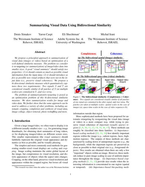
pˆjPˆjS(ource)completenesspiPiQˆjcoherenceFigure 3. Notations for the update rule.T(arget)qQicolor. We first isolate the contribution of the color of eachpixel q ∈ T to the error d(S, T ) of Eq. (1).The error a pixel q ∈ T contributes to d cohere (S, T ):Let Q 1 , . . . , Q m denote all the patches in T that containpixel q (e.g., if our patches are 7 × 7, there are 49 suchpatches). Let P 1 , . . . , P m denote the corresponding (mostsimilar) patches in S (i.e., P i = arg min P ⊂S D(P, Q i )).Let p 1 , . . . , p m be the pixels in P 1 , . . . , P m correspondingto the position of pixel q within Q 1 , . . . , Q m (see Fig. 3).Then 1 ∑ mN T i=1 (S(p i) − T (q)) 2 is the contribution of thecolor of pixel q ∈ T to the term d cohere (S, T ) in Eq. (1).The error a pixel q ∈ T contributes to d complete (S, T ):Let ˆQ1 , . . . , ˆQ n denote all the patches in T that containpixel q and serve as “the most similar patch” tosome patches ˆP 1 , . . . , ˆP n in S (i.e., ∃ ˆP j ⊂ S s.t. ˆQ j =arg min Q⊂T D( ˆP j , Q)). Note that unlike m above, whichis a fixed number for all pixels q ∈ T , n varies from pixel topixel. It may also be zero if no patch in S points to a patchcontaining q ∈ T as its most similar patch. Let ˆp 1 , . . . , ˆp nbe the pixels in patches ˆP 1 , . . . , ˆP n corresponding to theposition of pixel q within ˆQ 1 , . . . , ˆQ n (see Fig. 3). Then1N S∑ nj=1 (S(ˆp j) − T (q)) 2 is the contribution of the colorof pixel q ∈ T to the term d complete (S, T ) in Eq. (1).Thus, the overall contribution of the color of pixel q ∈ Tto the global bidirectional error d(S, T ) of Eq. (1) is:1Err(T (q)) =n∑N Sj=1(S(ˆp j ) − T (q)) 2 + 1N Tm∑i=1(S(p i ) − T (q)) 2 . (4)To find the color T (q) which minimizes the error in Eq. (4),Err(T (q)) is differentiated w.r.t. the unknown color T (q)and equated to zero, leading to the following expression forthe optimal color of pixel q ∈ T (the Update Rule):T (q) =1N Sn∑j=1S(ˆp j ) + 1N Tm∑S(p i )i=1nN S+ m (5)N TThis entails a simple iterative algorithm. Given the targetimage T (l) obtained in the l-th iteration, we compute thecolors of the target image T (l+1) as follows:1. For each target patch Q ⊂ T (l) find the most similarsource patch P ⊂ S (minimize D(P, Q)). Colors of pixelsin P are votes for pixels in Q with weight 1/N T .2. In the opposite direction: for each ˆP ⊂ S find themost similar ˆQ ⊂ T (l) . Pixels in ˆP vote for pixels in ˆQwith weight 1/N S .3. For each target pixel q take weighted average of allits votes as its new color T (l+1) (q). (Color votes S(p i ) arefound in step 1, S(ˆp i ) in step 2.)3.2. Convergence by Gradual ResizingAs in any iterative algorithm with a non-convex errorsurface, the local refinement process converges to a goodsolution only if the initial guess is “close enough” to thesolution. But what would be a good initial guess in thiscase? Obviously the “gap” in size (and hence in appearance)between the source image S and the target image Tis too large for a trivial initial guess to suffice: A randomguess would be a bad initial guess of T ; Simple croppingof S to the size of T cannot serve as a good initial guess,because most of the source patches would have been discardedand would not be recoverable in the iterative refinementprocess; Scaling down of S to the size of T is not agood initial guess either, because the appearance of scaleddownpatches is dramatically different from the appearanceof source patches, preventing recovery of source patches inthe iterative refinement process.If, on the other hand, the “gap” in size between thesource S and target T were only minor (e.g., |T | = 0.95|S|,where | · | denotes the size), then subtle scaling down of thesource image S to the size of T could serve as a good initialguess (since all source patches are present with minorchanges in appearance). In such an “ideal” case, iterativerefinement using the update rule of Eq. (5) would convergeto a good solution.Following this logic, our algorithm is applied through agradual resizing process, illustrated in Fig. 4. A sequenceof intermediate target images T 0 , T 1 , . . . , T K of graduallydecreasing sizes (|S| = |T 0 | > |T 1 | > ... > |T K | = |T |)is produced, where T 0 = S. For each intermediate targetT k (k = 1, . . . , K) a few refinement iterations are performed.The target T k is first initialized to be a scaled-downversion of the previously generated (and slightly larger)target T k−1 , i.e., T (0)k:= scale down(T k−1 ). Then iterativerefinement is performed using the update rule ofEq. (5) until convergence is obtained for the k-th target size:T (L)k= arg min d(S, T k ). This gradual resizing guaranteesthat at each intermediate output size (k = 1, . . . , K) theinitial guess T (0)kis always close to the desired optimumof T k , thus guaranteeing convergence at that output size.Note that the bidirectional distance measure d(S, T k ) is alwaysminimized w.r.t. the original source image S (andnot w.r.t. to the previously recovered target T k−1 ), sincewe want to obtain a final desired output summary T = T Kthat will minimize d(S, T ). An example sequence of im-

InputSscaledownT 1 T 2 T KT(0)1 T(1)iterate1 T(L)scaleiterate1 T(0)2 T(1)2 T(L)Eq.(5) downEq.(5) 2. . .T(0) K T(1)iterateK T(L)Eq.(5) KOutputTmin d(S, T 1 )min d(S, T 2 )min d(S, T K )Figure 4. Gradual resizing algorithm. Target size is gradually decreased until it reaches the desired dimensions. For each intermediateoutput T k (k = 1, . . . , K) the iterations T (0)k, . . . , T (L)k(inside blue rectangles) are initialized by scaling down the final result of theprevious output: T (L)k−1. Fig. 5 shows intermediate outputs in such gradual resizing. Please view video in www.wisdom.weizmann.ac.il/ ∼ vision/VisualSummary.html.d (S,T k ) T 8Source = T 0 T 1 T2T 7T 2 TT 6 3 T T 4 T 55 T6T 7 T 8d(S,T 0 )= 0 d(S,T 1 ) = 175 d(S,T 2 ) = 345 d = 504 d = 597 d = 640 d = 980 1408 2150Figure 5. Gradual image resizing. Results of our algorithm for gradually decreasing target size, with corresponding dissimilarity valuesd(S, T ) given by Eq. (1). Note that when the target size is so small that we must compromise completeness (such as in T 6, T 7, T 8, whereis not enough space to contain all source patches), the algorithm still preserves coherence. It selects the most coherent result among theequally incomplete ones.age summaries of gradually decreasing sizes is shown inFig. 5. Please view video in www.wisdom.weizmann.ac.il/ ∼ vision/VisualSummary.html.This gradual resizing procedure is implemented coarseto-finewithin a Gaussian pyramid (spatial in the case of images,spatio-temporal in the case of videos). Such a multiscaleapproach allows to escape local minima and speeds upconvergence, having a significant impact on the results.4. Results and ApplicationsOur similarity measure (Sec. 2) and retargeting algorithm(Sec. 3) can be used for a variety of applications.Results are shown below for image/videosummarization, image montage, image synthesis, photoreshuffling, and automatic cropping. Video resultscan be found in www.wisdom.weizmann.ac.il/∼ vision/VisualSummary.html.Image Summarization: Figs. 5 shows results of ourgradual resizing algorithm (Sec. 3) and the correspondingsimilarity measure d(S, T ) of Eq. (1). In the first few images,T 1 , ..., T 5 , the loss of visual information is gradual, accompaniedby a slow increase in the dissimilarity measured(S, T ). Starting from T 6 a significant amount of visualinformation is lost from image to image, which is also supportedby a sharp increase in d(S, T ) (see graph in Fig. 5).This may suggest an automatic way to identify a good stoppingpoint in the size reduction. Developing such a criterionis part of our ongoing work.Fig. 6 presents results of image summarization obtainedwith our algorithm (Sec. 3) for several input images andfor several different output sizes. It shows how the algorithmperforms under different space limitations, down tovery small sizes. These results are compared side-by-sidewith the output of the “Seam Carving” [1] algorithm 2 .Our algorithm exploits redundancy of image patterns(e.g., the windows in the building) by mapping repetitivepatches in the source image to a few representative patchesin the target image (as in “Epitome” [4, 7]), thus preservingtheir appearance at the original scale. “Seam Carving” [1]removes vertical and horizontal paths of pixels with smallgradients, nicely shrinking large images as long as thereare enough low-gradient pixels to remove. It first removesuniform regions (such as the sky in the building image ofFig. 6), while maintaining faithful appearance of all objectsin the image. However, when the image gets too small andall low-gradient pixels have been removed, “Seam Carving”starts distorting the image content. Moreover, since its decisionsare based on pixel-wide seams, it does not try to preservelarger image patterns, nor does it exploit redundancyof such patterns. As such, it is less adequate for highlystructured images (like images of buildings). Please viewvideo on demo website, exemplifying these behaviors.Our algorithm as described in Sec. 3 is significantlyslower than “Seam Carving”. However, the computationallyheavy nearest-neighbor search may be significantly2 Code from http://www.thegedanken.com/retarget.

Input imageInput imageInput imageInput imageInput imageour methodseam carvingour method seam carvingour method seam carvingour method seam carvingour method seam carving Wolf et al.pure scalingFigure 6. Image summarization results. Our method exploits redundancies in the images (bushes, waves, windows of the buildings, etc.),often creating coherently-looking images even for extremely small target sizes. “Seam Carving” prefers to remove low-gradient pixels,thus distorts the image considerably at small sizes, when there are no more low-gradient pixels left. Please view video on demo website.The Dolphin image is from Avidan and Shamir [1], the right-most building image from Wolf et al. [16].sped up by using location from previous iteration to constrainthe search. Our current implementation in Matlabtakes 5 minutes to resize 250×200 to half its size, and scaleslinearly with the image size. Our algorithm can be parallelizedon multiple CPU’s/GPU for significant speedup.After pure image scaling objects may become indiscernibleif significantly scaled down, or distorted if the aspectratio changes substantially from source to target (seean example in Fig. 6). The importance-based retargetingmethods of [10, 14, 16] give very nice results when there arefew “important” objects within an image, but reduce to pureimage scaling in case of uniform importance throughout theimage. For instance, in the right-most example in Fig. 6,the result of Wolf et al. [16] is very similar to pure imagescaling. In Sec. 5 we further describe how non-uniform importancecan also be incorporated into our summarizationalgorithm, and present comparison to Wolf et al. [16] onone of their examples containing faces.Note that most existing summarization algorithms(e.g., [1, 14, 16, 3, 15, 10, 12, 8, 17]) cannot exploit repetitivenessor redundancy of the visual data. This leads tosignificant scaling down or distortion of image patterns bythese methods when the target size gets very small.Image/Video Montage. Image Tapestry/AutoCollage(e.g., [13]) and Video Montage (e.g., [8]) address the followingproblem: Given a set of inputs S 1 , S 2 , ..S n (imagesor videos), merge them into a single output T (imageor video) in a seamless “sensible” way. Our algorithmof Sec. 3 can be applied to produce an image/videomontage by taking multiple images/videos as a source (i.e.,S = {S 1 , S 2 , ..S n }). An example result is shown in Fig. 7.Input 2 Input 3Input 1Output montageFigure 7. Image montage result. Three different input imageswere automatically merged into a single output in a seamless coherentway. Simple side-by-side stacking of the three input imageswas taken as an initial guess, and then gradually resized to thetarget montage size using our algorithm from Sec. 3.InputBigger output (Synthesis)Figure 8. Synthesis results. (See text for details.)Completeness guarantees that all patches from all input imagesare found in the output montage, while the coherenceterm guarantees their coherent merging. Note that no graphcutnor post-processing blending has been used in this case.

Reshuffle 1 Reshuffle 2InputOutput(a) Input image (b) Bidirectional (c) Detectedsimilarity map optimal croppingFigure 9. Photo reshuffling. The user specifies new locations ofobjects (man and ox, girl and bench). The rest of the image isreconstructed in the most complete and coherent way.Source video. . .. . .Target video(½ length)Figure 10. Video summarization result. A complex ballet videosequence was summarized to half its temporal length by our algorithm(Sec. 3). Please view video on demo website.Image/Video Completion and Synthesis: In data synthesis/completion(e.g., [6, 18]), the new synthesized regionsmust be visually coherent with respect to the input data. Bysetting α = 0 in Eq. (2), our similarity measure reduces tothe Coherence objective function of [18], and our optimizationalgorithm of Sec. 3 reduces to a synthesis algorithmsimilar to that of [18]. An example of an image synthesisresult can be found in Fig. 8.Photo reshuffling: We used our algorithm to reshuffle visualinformation according to user guidance (see Fig. 9).The user roughly marks objects and specifies their desiredlocations in the output. We then apply our similarityoptimizationalgorithm (Sec. 3) to fill in the remaining partsof the image in the most complete and coherent way. Adifferent approach for photo-reshuffling appears in [5].Video results: We further applied our optimization algorithmto generate a visual summary of video data (whereS and T are video clips, and the patches are space-timepatches at multiple space-time scales). We summarized acomplex ballet video clip S by a shorter target clip T ofhalf the temporal length – see Fig 10. The resulting outputclip, although shorter, is visually coherent – it conveys a visuallypleasing summary of the ballet movements at theiroriginal speed! On the other hand, it is also complete inthe sense that it preserves information from all parts of thelonger source video. Please view video on demo website,showing the input sequence and the resulting shorter outputsequence (the video summary).Automatic Cropping: The bidirectional measure describedin Sec. 2 allows for automatic extraction of the best windowto crop. Let S be the input image, and let T be theFigure 11. Automatic optimal cropping. (a) Input images.(b) The bidirectional similarity measure maps color coded fromblue (low similarity) to red (high similarity). The white circlesmark the highest peaks and the white rectangles mark the correspondingbest windows to crop. (c) The detected optimal cropping.(unknown) desired cropped region of S, of predefined dimensionsm × n. Sliding a window of size m × n acrossthe entire image, we compute the bidirectional similarityscore of Eq. (1) for each window, and assign it to its centerpixel. This generates a continuous bidirectional similaritymap for S – see Fig. 11.b. The peak of that map is the centerpixel of the best window to crop in order to maintainmaximal information (note that in this case only the “completeness”term will affect the choice, since all sub windowsof S are perfectly “coherent” with respect to S). Often thereis no single “good” place to crop (see lower row of Fig. 11).In that case the bidirectional similarity map contains multiplepeaks, which can serve as multiple possible locations tocrop the image (with their relative scores).The same approach was used for temporal cropping invideo data, using our bidirectional similarity measure withspace-time patches. View video on the project website.5. Incorporating Non-Uniform ImportanceSo far we assumed that all image regions are equally important.Often, however, this is not the case. For example,people are often more important than other objects. Suchnon-uniform importance is exploited in many retargetingand auto-cropping methods (e.g., [8, 11, 12, 14, 15, 16]).Non-uniform importance can be incorporated into our bidirectionalsimilarity measure by introducing “importanceweights” in Eq. (1):d(S, T ) =∑w P · min D(P, Q)Q⊂T∑P ⊂S w +PP ⊂S∑Q⊂Tw ˆP · minP ⊂S D(Q, P )∑Q⊂T w ˆPwhere w P is the patch importance weight and ˆP =arg min P ⊂S D(Q, P ). Note that the weights in both com-(6)

Input imageOur summarywithout weightsOur summarywith weightsImportance weightsWolf et al.(with weights)6. ConclusionWe proposed a bidirectional similarity measure betweentwo images/videos of different sizes. We described a principledapproach to retargeting and summarization of visualdata (images and videos) by optimizing this bidirectionalsimilarity measure. We showed applications of this approachto image/video summarization, data completion andremoval, image synthesis, image collage, photo reshufflingand auto-cropping.Acknowledgments The authors would like to thankLena Gorelick and Alex Rav-Acha for their insightful commentson the paper. This research was supported in part bythe Israeli Ministry of Science.Figure 12. Incorporating non-uniform importance. Withoutweights (left) our method prefers to preserve textured regions (e.g.,books) over semantically important regions (e.g., faces). Importanceweights on the faces solve this problem (center). Correspondingresult of Wolf et al. [16] is shown on the right (the maskthey used for this result may be different from ours). Note that theface of the girl has been preserved better with our method.Input Importance mask OutputsFigure 13. Summarization with object removal constraints.White = high weights, black = low weights. This guarantees thatthe bungee jumper will not be included in the visual summary. Noaccurate segmentation is needed. Visual summaries of differentsizes are shown.pleteness and coherence terms (w P and w ˆP, respectively)are defined over the source image.Fig. 12 illustrates the contribution of using importanceweights. Without importance weights, our method prefersthe textured regions (e.g., the books) over the relatively homogeneousregions (e.g., the faces), which may be semanticallymore important. Introduction of importance weightssolves this problem. Fig. 12 also includes comparison to theimportance-based method of [16].Importance weights can further be used to remove/eliminateundesired objects from the output image inthe summarization process, as shown in Fig. 13.References[1] S. Avidan and A. Shamir. Seam carving for content-awareimage resizing. SIGGRAPH, 2007.[2] O. Boiman and M. Irani. Similarity by composition. In NIPS,pages 177–184, Vancouver, BC, Canada, 2007.[3] L.-Q. Chen, X. Xie, X. Fan, W.-Y. Ma, H.-J. Zhang, and H.-Q. Zhou. A visual attention model for adapting images onsmall displays. Multimedia Systems, 2003.[4] V. Cheung, B. J. Frey, and N. Jojic. Video epitomes. IJCV,Dec 2006.[5] T. S. Cho, M. Butman, S. Avidan, and W. T. Freeman. Thepatch transform and its applications to image editing. InCVPR, 2008. To appear.[6] A. A. Efros and T. K. Leung. Texture synthesis by nonparametricsampling. In ICCV, pages 1033–1038, 1999.[7] N. Jojic, B. J. Frey, and A. Kannan. Epitomic analysis ofappearance and shape. In ICCV, 2003.[8] H.-W. Kang, Y. Matsushita, X. Tang, and X.-Q. Chen. Spacetimevideo montage. In CVPR (2), 2006.[9] A. Kannan, J. Winn, and C. Rother. Clustering appearanceand shape by learning jigsaws. NIPS, 2006.[10] F. Liu and M. Gleicher. Automatic image retargeting withfisheye-view warping. In UIST, 2005.[11] F. Liu and M. Gleicher. Video retargeting: Automating panand-scan.ACM Multimedia 2006, October 2006.[12] A. Rav-Acha, Y. Pritch, and S. Peleg. Making a Long VideoShort. In CVPR, June 2006.[13] C. Rother, L. Bordeaux, Y. Hamadi, and A. Blake. Autocollage.SIGGRAPH, 25(3):847–852, 2006.[14] V. Setlur, S. Takagi, R. Raskar, M. Gleicher, and B. Gooch.Automatic image retargeting. In MUM, 2005.[15] B. Suh, H. Ling, B. B. Bederson, and D. W. Jacobs. Automaticthumbnail cropping and its effectiveness. In UIST,2003.[16] L. Wolf, M. Guttmann, and D. Cohen-Or. Non-homogeneouscontent-driven video-retargeting. In ICCV’07.[17] Y.Pritch, A.Rav-Acha, A.Gutman, and S.Peleg. Webcamsynopsis: Peeking around the world. In ICCV, 2007.[18] Y.Wexler, E. Shechtman, and M. Irani. Space-time completionof video. PAMI, 27(2), March 2007.