solar cycle effects on gnss-derived ionospheric total electron content ...

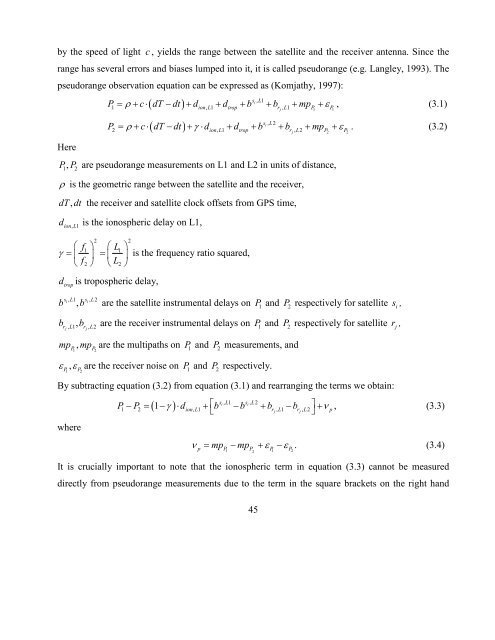
y the speed of light c , yields the range between the satellite and the receiver antenna. Since therange has several errors and biases lumped into it, it is called pseudorange (e.g. Langley, 1993). Thepseudorange observation equation can be expressed as (Komjathy, 1997):Heresi, L1( ) ion L trop rjL Pε1 P1P = ρ + c ⋅ dT − dt + d + d + b + b + mp + , (3.1)1 , 1 , 1si, L2( ) ion L trop rjL P2 P2P = ρ + c ⋅ dT − dt + γ ⋅ d + d + b + b + mp + ε . (3.2)2 , 1 , 2P1 , P2are pseudorange measurements on L1 and L2 in units of distance,ρ is the geometric range between the satellite and the receiver,dT,dt the receiver and satellite clock offsets from GPS time,dion, L1is the ionospheric delay on L1,2 2⎛ f ⎞ ⎛1L ⎞1γ = ⎜ ⎟ = ⎜ ⎟ is the frequency ratio squared,f L⎝ 2 ⎠ ⎝ 2 ⎠dtropis tropospheric delay,si, L1 si, L2b , b are the satellite instrumental delays on1rj, L1 rj, L245P and P2respectively for satellite si,b , b are the receiver instrumental delays on P1and P2respectively for satellite rj,mp , mp are the multipaths on P1and P2measurements, andP1 P2ε , ε are the receiver noise on P1and P2respectively.P1 P2By subtracting equation (3.2) from equation (3.1) and rearranging the terms we obtain:where( γ )P − P = − ⋅ d + ⎡b − b + b − b ⎤ +⎣⎦si , L1 si, L21 21ion, L1 rj, L1 rj, L2νpp P1 P P2 1 P2, (3.3)ν = mp − mp + ε − ε .(3.4)It is crucially important to note that the ionospheric term in equation (3.3) cannot be measureddirectly from pseudorange measurements due to the term in the square brackets on the right hand