Part 13- Simple linear regression - The University of Jordan

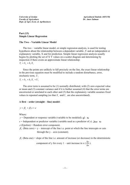
University of Jordan Agricultural Statistic (605150)Faculty of AgricultureDr. Amer SalmanDept. of Agri. Econ. & AgribusinessPart (13)Simple Linear RegressionThe Two – Variable Linear ModelThe two – variable linear model, or simple regression analysis, is used for testinghypothesis about the relationship between a dependent variable ,Y and an independent orexplanatory variable, X and for prediction. Simple linear regression analysis usuallybegins by plotting the set of X Y values on a scatter diagram and determining byinspection if there exists an approximate linear relationship:= b + b XYio 1iSince the points are unlikely to fall precisely on the line, the exact linear relationshipin the previous equation must be modified to include a random disturbance, error,stochastic term, UY X + Ui= bo+ b1iiiThe error term is assumed to be (1) normally distributed, with (2) zero expected valueor mean and (3) constant variance and if it is further assumed (4) that the error terms areuncorrected or unrelated to each other and (5) that the explanatory variable assumes fixedvalues in repeated sampling (so that X andU are also uncorrolated).A first – order (straight – line) model:= β + β x + εyo 1iWhere:متغير تابع modeled). y = Dependent or response variable (variable to beمتغير مستقل y). x = Independent or predictor variable (variable used as a predictor ofε (Epsilon) = Random error component.βo(Beta zero) = y – intercept of the line i.e. point at which the line intercepts or cutsthrough the y – axis (constant).β1(Beta one) = slope of the line i.e. amount of increase (or decrease) in the deterministic∆ ycomponent of y for every 1 – unit increase in x ( ).∆xi- 1 -

University of Jordan Agricultural Statistic (605150)Faculty of AgricultureDr. Amer SalmanDept. of Agri. Econ. & AgribusinessY32β1= slope1β = y - Intercepto0 X1 2 3 4 5Example (13 – 1):Y = tomato productionX = fertilizer quantityY = 10 + 2xتمثل الإنتاج في حالة عدم إضافة أي كمية من السماد :10نسبة الزيادة في الإنتاج عند إضافة وحدة واحدة من السماد ‏(إنتاجية الوحدة الواحدة من السماد ( :2Yβ1= slope =2β = 10o0 X1 2 3 4 5ˆ = ˆ β + ˆ β xyo 1قيمة الإنتاج المقدرة ‏(المتوقعة ( = ŷβˆ o ,1ˆβ = estimated population parametersˆ = β + β xyo 1- 2 -

University of Jordan Agricultural Statistic (605150)Faculty of AgricultureDr. Amer SalmanDept. of Agri. Econ. & Agribusinessβ∑∑x y1=2xx = X − Xy = Y − YFitting the model: the Method of Least SquaresSuppose that we have the following equation:y ˆ = −1+xx y ŷ ( y − yˆ)2( y − yˆ)(SSE)1 1 0 (1 – 0) = 1 12 1 1 (1 – 1) = 0 03 2 2 (2 – 2) = 0 04 2 3 (2 – 3) = -1 15 4 4 (4 – 4) = 0 0Sum of errors = 0 Sum of Squared errors = 2Y3y ˆ = −1+x210-11 2 3 4 5XIt can be shown that there is one (and only one) line for which the SSE is a minimum.This line is called the least square line, the regression line, the least squares equation orthe fitted line.- 3 -

Ça bouge en villeJusqu’au 23 avril, durantles travaux pour la constructiond’un bassin d’orage, il n’est paspossible de stationnerdans la rue de la Roselière et lavitesse est limitée à 30 km/h.Rue de Mulhouse (tronçon ruede Séville - rue de l’Aéroport),du 14 mars au 31 mai, la vitessesera limitée à 30 km/h etle stationnement sera interditpour cause de réaménagementde trottoirs.Le renouvellement du réseaugaz continue sur l’avenue Généralde Gaulle et rue de l’Horticulture.Avenue Général de Gaulle,la vitesse est limitée à 30 km/h.Rue de l’horticulture,la circulation est interdite, saufpour les riverains. Il n’est paspossible de se stationner.Rue de l’Église, les travauxconcernent le réseau électriquebasse tension et la voirie. Lestationnement et la circulationsont interdits pendant les travaux.Les rues du Jura et des Alpes sont de nouveau praticables.Rues du Jura et des AlpesToutes neuves !Démarrés en novembre, les travaux devoirie des rues du Jura et des Alpessont sur le point d’être finis. Ce chantierentre dans le programme de voirie2010. 220 000 € TTC ont été nécessairepour refaire entièrement les chaussées.“Elles en avaient besoin et laconstruction du commissariat de policea été l’occasion de lancer le chantier”,affirme Bernard Schmitter, adjointà l’urbanisme et à la voirie de la villede Saint-Louis. Les chaussées, surenviron 400 mètres linéaires, ont étédécaissées sur 50 cm de profondeur.Un film géotextile a été posé, puis unecouche de gravier et une couche degraves fines. La touche finale a été letapis d’enrobés, posé tout récemment.L’éclairage public et les trottoirs ontégalement été refaits.Opération nids de pouleLa légère accalmie climatique de mijanviera permis aux services de laVille, avec l’appui d’une entreprise privée,de traiter un grand nombre detrous en formation sur près de 30 rues.En effet, le gel et le sel avaient fortementdégradé les chaussées. À l’heureactuelle, tous les nids de poules ontété rebouchés. Les riverains sont invitésà signaler en mairie (services techniques)les nouveaux nids de poulesdès formation de ceux-ci.Ici, les nids de poulesde la rue Baerenfelsont été rebouchés.5 À l’action

University of Jordan Agricultural Statistic (605150)Faculty of AgricultureDr. Amer SalmanDept. of Agri. Econ. & AgribusinessTable (13 – 2):n Y (corn)iXi(fertilizer) ( Y i− Y )yi( X i− X )xi( x y ) 2i i x1 40 6 -17 -12 204 1442 44 10 -13 -8 104 643 46 12 -11 -6 66 364 48 14 -9 -4 36 165 52 16 -5 -2 10 46 58 18 1 0 0 07 60 22 3 4 12 168 68 24 11 6 66 369 74 26 17 8 136 6410 80 32 23 14 322 196n = 10 Y =570 X =180 y =0 x =0 ∑ i i ∑ x 2 i=576∑ iY = 57∑ iX = 18∑ i∑ iiTable (13 – 2) shows the calculation to estimate the regression equation for the corn –fertilizer problem in table (1) using the equation:ˆxiyi956bi= = 1.66 (The slope of the estimate regression line)2x 576=∑∑ibˆˆo= Y − b X ≅ 57 − (1.66)(18) = 57 − 29.88 27.12 (The Y – Intercept)1≅Yˆ = 27.12 + 1. 66 (The estimated regression equation)iX iThus when X i= 0, Yˆ i = 27.12, X = Xi=18, Yˆ i = 27.12 + 1.66 (18) =57 = Y as a result, theregression line passes through point X Y .- 6 -

University of Jordan Agricultural Statistic (605150)Faculty of AgricultureDr. Amer SalmanDept. of Agri. Econ. & AgribusinessYŶ iβ1= 1.66β = 27.12oXExample (13 – 3):X Y ( Y i− Y )∑ iiiyi( X i− X )xi( x y ) 2i i x1 1 -1 -2 2 42 1 -1 -1 1 13 2 0 0 0 04 2 0 1 0 15 4 2 2 4 4X =15 Y = 10 y =0 x =0 ∑ xiyi=7 ∑ x 2 i=10X = 3∑ iY = 2∑ i∑ iib ˆˆib o=∑∑x7=10i i=2ixy= Y − bˆX0.7= 2 − (0.7)(3) =1−0.1Y ˆ = −0.1+ 0. 7iX i- 7 -

University of Jordan Agricultural Statistic (605150)Faculty of AgricultureDr. Amer SalmanDept. of Agri. Econ. & AgribusinessY0.7-0.1XExample (13 – 4):Yˆ= 10 − 5Xβ = 10oYβ1= -5XExample (13 – 5):Yˆ= −10− 5X- 8 -

University of Jordan Agricultural Statistic (605150)Faculty of AgricultureDr. Amer SalmanDept. of Agri. Econ. & AgribusinessYXβ = -10oβ1= -5Test of Significance of Parameter EstimatesIn order to test for statistical significance of the parameter estimates of the regressionthe variance ofbˆ o and ˆb 1is required.∑∑2var ˆx2 ibo= σu 2n xˆ 2 1varb = σu 2x∑1LiiL(1)(2)s2Sinceσ2 uis unknown, the residual variance s 2 2is used as an (unbiased) estimate ofσ u:22ˆ∑ei= σu= L(3).(Where k = number of parameter estimates).n − kUnbiased estimates of the variance ofbˆ o and ˆb 1are then given by:∑2222∑∑ ∑2 ˆ = eixi×⇒ ˆ ei(4) =−−× xiS boL S b2on k n xn k n x2∑e i= ( Y − Yˆ)n = number of observations.k = number of parameters.i∑i- 9 -

University of Jordan Agricultural Statistic (605150)Faculty of AgricultureDr. Amer SalmanDept. of Agri. Econ. & Agribusiness∑22ei1∑×⇒ ˆei(5) S b =− ∑−×21n k xin k ∑2 bˆ1= 12xiS LSo that S b ˆ o and S ˆb 1are the standard errors of the estimates. SinceU iis normallydistributed, Yiand therefore bˆ o and ˆb 1are also normally distributed, so that we can use thet distribution with n – k degrees of freedom, to test hypotheses about and constantconfidence intervals forbˆ o and ˆb 1.tocalbo− bo= ˆSbo,t1calbˆ1− b=Sb11df = n – k (n – 2 always).α = 5 %; one tailed (α), two tailed (α/2).Example (13 – 6):The following table shows the calculations required to test the statistical significanceofbˆ o and ˆb 1. The value of Yˆ iin the table are obtained by subtracting the values of Xiintothe estimated regression equation Yˆ 2i= 27.12 + 1. 66Xi(The values of yiare obtained bysquaring yi( Y i− Y ).Table (13 – 3):year Y (corn)iXi(fertilizer)Yˆ i( Y − Yˆ)e= i2ei2Xi2xi2yi2( Y i− Y )1 40 6 37.08 2.92 8.5264 36 144 2892 44 10 43.72 0.28 0.0784 100 64 1693 46 12 47.04 -1.04 1.0816 144 36 1214 48 14 50.36 -2.36 5.5696 196 16 815 52 16 53.68 -1.68 2.8224 256 4 256 58 18 57.00 1.00 1.0000 324 0 17 60 22 63.64 -3.64 13.2496 384 16 98 68 24 66.96 1.04 1.0816 576 36 1219 74 26 70.28 3.72 13.8384 676 64 28910 80 32 80.24 -0.24 0.0576 1,024 196 529n=10∑Y i=570Y =57∑ iX =180X =18∑ ie =0∑e2 i=47.3056∑ X2i=3,816∑ x2 i=576∑ y2 i=1,634- 10 -

University of Jordan Agricultural Statistic (605150)Faculty of AgricultureDr. Amer SalmanDept. of Agri. Econ. & AgribusinessS2bˆS bˆoo∑2ei= ×n − k n∑∑x= 3.92 = 1.982ix2i=47.3056×10 − 2381610(576)= 3.922S bˆ=S bˆ11∑2ei×n − k∑1x= 0.01 ≅ 0.12i47.3056=≅ 0.01(10 − 2)(576)bˆo− bo27.12 − 0bˆ1− b11.66 − 0Therefore, tocal= = ≅ 13. 7 and t1 = = = 16. 6Sbˆ1.98calSb 0.1Since bothtocaltandot 1 calexceed t tabsignificance we [ t t ]= 2.306 with df = n – k = 8 at 5 % level ofo,1>cal cal tabconclude that bothb 0.025oand b 1are significant at the 5 %level of significance (two tailed).1RejectionRegionAcceptance RegionRejection Regiont =2.306tab α /2t =2.306 13.7 16.6tab α /2- 11 -

University of Jordan Agricultural Statistic (605150)Faculty of AgricultureDr. Amer SalmanDept. of Agri. Econ. & AgribusinessA Test of Model UsefulnessTable (13 – 4):One tailed testH : β = 0 1Hoa: β1 < 0, or Ha: β1>Test statistic = t0ˆ β − βS ˆ β1ˆ β − βS ˆ βoTwo tailed testH : β = 0 1Hoo: β1 ≠ 01 1o o1= , to=Test statistic = t1Rejection region t < −tα, or t > tWheret αis based on (n – 2) dfαˆ β1− β1= , tS ˆ β1oˆ βo− βo=S ˆ βRejection region t < −tα/ 2, or t > tα/ 2Wheret αis based on (n – 2) dfFor example (13 – 3), we will choose α = 0.05 and, since n = 5, df = (n – 2) = 3, then therejection region for the two tailed test is:t < −t= − .182, or t > t 3.1820 .02530. 025=os2=SSEn − k=SSEn − 2Where:2SSE ( yi− yˆ ) = SSyy− ˆ β1SS∑=xy∑( y − y)2∑( ∑ yi)2SSyy=i= yi−n2 1.10s = = 0.367 ⇒ s = 0.367 = 0.613We estimated previously 1ˆβ = 0.7, s = 0.61 and SSThus:βt =s / SSxx0.7 0.7= =0.61/ 10 0.19ˆ1 =23.7xx( x )222 ∑ i (15)= ∑ xi− = 55 − = 10n5- 12 -

University of Jordan Agricultural Statistic (605150)Faculty of AgricultureDr. Amer SalmanDept. of Agri. Econ. & AgribusinessRejectionRegionRejectionRegionttab =-3.182ttab =3.182 tcal= 3.7ttab < tcal ; 3.182 < 3.7Since the calculated t value falls in the upper – tail rejection region we reject the nullhypothesis and conclude that the slope of1ˆβ is not 0 and it is significant at 5 % level ofsignificance.Another way to make inference about the slope of1ˆβ is not estimate it using aconfidence interval as follows:ˆ ˆsβ1± tα / 2Sβ1When S βˆ = , and tα / 2is based on (n – k) df.SS xxˆ ˆ⎛ 0.61⎞β1 ± tα / 2Sβ1= 0.7 ± 3.182⎜⎟ = 0.7 ± 0.61⎝ 10 ⎠Thus we estimate with 95 % confidence that the interval from 0.09 to 1.31 includes theslope parameter β1. We would expect a narrower interval if the sample size wereincreased.Test of Goodness of Fit and CorrelationThe closer the observations fall to the regression line (i.e. the smaller the residuals),the greater is the variation in Y “explained” by the estimated regression equation. Thetotal variation in Y is equal to the explained plus the residual variation:- 13 -

University of Jordan Agricultural Statistic (605150)Faculty of AgricultureDr. Amer SalmanDept. of Agri. Econ. & Agribusiness22222 2( Y − Y ) = ( Yˆ− Y ) + ( Y − Yˆ) ,[ y = yˆe ]∑ i ∑ i i ∑ i i ∑ i ∑ i+ ∑Total variation = Explained variation + Residual variationIn Y (or total in Y (or regression in Y (or errorSum of squares) sum of squares) sum of squares)TSS = RSS + ESSDividing both sides by TSS:RSS ESS1 = +TSS TSS2The coefficient of determination or R is then defined as the proportion of the totalvariation in Y explained by the regression of Y on X.iR2RSS= = 1−TSSESSTSS2R Can be calculated by:R2∑∑∑∑22= yˆiei= 1−2y y2ii∑∑Where: y ˆ = ( − ) 2iYiYi22∑ei= ∑ ( Y i− Yˆi)22∑ yi= ∑ ( Yi− Y )2 ˆ2R Ranges in value from 0 (zero when the estimated regression equation explains nonof the variation in Y) to 1 (when all points lie on the regression line).The Correlation Coefficient:rThe correlation coefficient is given by:∑ x2 iyi∑== ˆxiyiRb12 2x y yi=2∑i∑i∑- 14 -

University of Jordan Agricultural Statistic (605150)Faculty of AgricultureDr. Amer SalmanDept. of Agri. Econ. & Agribusinessr ranges in value from -1 (for perfect negative linear correlation) to +1 (for perfectpositive linear correlation) and dose not imply causality or dependence.Example (13 – 7):The coefficient of determination for the corn – fertilizer example can be found from:R2=∑∑e2i1−2yi47.31≅ 1−= 1−0.0290 = 0.9710 ≅ 97.10%1634Thus the regression equation about 97 % of the total variation in corn output, theremaining 3 % is attributed to factors included in error term. Then:2r = R = 0.971 = 0.9854 Or 98.54 % and is positive because ˆb 1is positive.Example (13 – 8):nXiYixiX i− XyiY i− Yxiy i2xiŶi2ei( Y ) 2i− Yˆiy22Xii1 1 1 -2 -1 2 4 0.6 0.16 1 12 2 1 -1 -1 1 1 1.3 0.09 4 13 3 2 0 0 0 0 2 0 9 04 4 2 1 0 0 1 2.7 0.49 16 05 5 4 2 2 4 4 3.4 0.36 25 4n=5 ∑X =15iX =3∑ iY =2Y =10∑ ix =0ˆxiyi7β1= = 0.7 ,2x 10iˆ β ˆo= Y − β X = 2 − (0.7)(3) =Y ˆ = −0.1+ 0. 7x=∑∑2S ˆ β =S ˆ β =oo∑1−2ei×n − k n∑∑x2i2xi0.4033 = 0.6351.1= ×5 − 20.1∑ i555(10)y =0∑ =7 ∑ 2 ix i y i60.5= = 0.4033150x =10∑ 2 ie =1.1∑ 2 iX =55( Y Y ) 2i−∑ 2 iy =6- 15 -

University of Jordan Agricultural Statistic (605150)Faculty of AgricultureDr. Amer SalmanDept. of Agri. Econ. & Agribusiness2S ˆ β =S bˆ11=∑2ei×n − k∑1x2i0.03667 = 0.1911.1= ×5 − 2110= 0.03667obˆo− b=Sboo=− 0.1−0= −0.1570.635tcal66bˆ1− b= Sb0.7 − 0=0.19111=13.tcal025tα / 2 0.(Two tailed) at 5 % significance level, df (n – k) = (5 – 2) = 3ttab=3.182- t tabttabRejectHoAcceptHoRejectHo-3.182-0.157 0 3.182 3.66to calt 1 calt1; reject Ho , accept Ha ; t 1is significantto; accept Ho , reject Ha ; t ois insignificanttcal> t tabR2=r = R∑∑e2i1−2yi2=1.1≅ 1−= 0.816 ≅ 81.67%60.8167 = 0.9037- 16 -

University of Jordan Agricultural Statistic (605150)Faculty of AgricultureDr. Amer SalmanDept. of Agri. Econ. & Agribusinessxمعناه أن التغير الحاصل في yنتيجة التغير الحاصل فييمكن تفسيره بنسبة صحة مقدارها %81.67 والباقي يعزى إلى عوامل2Rأخرى.‏Example (13 – 9):The following table shows the relation between N (x) and Potato production (y). Find theregression equation and the coefficient of determination R 2 and sketch the curveaccording to your results.XiYixiX i− XyiY i− Yx y 2i i xiYˆi2ei( Y − Y ) 2iˆi2Xi2yi( Y Y) 2i−1 1 -2.5 -1.75 4.375 6.25 1.115 0.0313 1 3.0633 2 -0.5 -0.75 0.375 0.25 2.423 0.1759 9 0.5634 4 0.5 1.25 0.625 0.25 3.077 0.852 16 1.5636 4 2.5 1.25 3.125 6.25 4.385 0.1479 36 1.563X =3.5 Y =2.75 8.5 13 1.1923 6.75Yˆ= βo+ β1x ; β1= 0.654, βo= 0.461Yˆ = 0.461+0. 654x (Regression equation)Yβ 1β oX2∑ e < ∑R22iy i=∑∑e2i1−2yi1.1923≅ 1−= 0.8236.75- 17 -