Reconstruction using surface dedicated tensorial fields - ENSEA

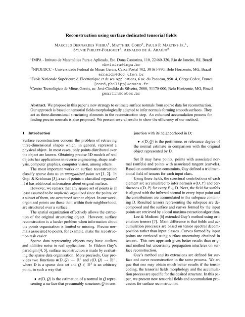
Reconstruction using surface dedicated tensorial fieldsMARCELO BERNARDES VIEIRA 1 , MATTHIEU CORD 3 , PAULO P. MARTINS JR. 4 ,SYLVIE PHILIPP-FOLIGUET 3 , ARNALDO DE A. ARAÚJO 21 IMPA - Intituto de Matemática Pura e Aplicada, Est. Dona Castorina, 110, 22460-320, Rio de Janeiro, RJ, Brazilmbvieira@impa.br2 NPDI/DCC - Universidade Federal de Minas Gerais, Caixa Postal 702, 30161-970, Belo Horizonte, MG, Brazilarnaldo@dcc.ufmg.br3 Ecole Nationale Supérieure d’Electronique et de ses Applications, 6 av. du Ponceau, 95014, Cergy Cedex, France{cord,philipp}@ensea.fr4 Centro Tecnológico de Minas Gerais, av. José Cândido da Silveira, 2000, 31170-000, Belo Horizonte, MG, Brazilpmartin@cetec.brAbstract. We propose in this paper a new strategy to estimate surface normals from sparse data for reconstruction.Our approach is based on tensorial fields morphologically adapted to infer normals forming smooth surfaces. Theyact as three-dimensional structuring elements in the reconstruction step. An enhanced accumulation process forfinding precise normals is also proposed. We present several results to show the efficiency of our method.1 IntroductionSurface reconstruction concern the problem of retrievingthree-dimensional shapes which, in general, represent aphysical object. In most cases, only points distributed overthe object are known. Obtaining precise 3D models of realobjects has applications in reverse engineering, shape analysis,computer graphics, computer vision, among others.The most important works on surface reconstructionclassify sparse data as an unorganized point set [1, 2]. InGopi & Krishman [3], a set of points is classified organizedif it has additional information about original surface.However, we remark that any sparse set of points is atleast assumed to be implicitly organized since the points, ora subset of them, are structured over an object. In our work,organized points are those that, within their neighborhood,are structured over a surface.The spatial organization effectively allows the extractionof the original structuring object. However, surfacereconstruction is a harder problem when information aboutthe points organization is limited or missing. Precise normalsassociated to points, for example, make the recostructiontask easier.Sparse data representing objects may have outliersand additive noise in real applications. In Gideon Guy’sparadigm [4, 5], surface reconstruction is made by evaluatingthe sparse data organization. More precisely, Guy providestwo functions n(D, Q) → R 3 and s(D, Q) → R + ,where D is a sparse data set and Q ∈ R 3 is an arbitrarypoint, in such a way that• n(D, Q) is the estimation of a normal in Q representinga surface that presumably structures Q in conjunctionwith its neighborhood in D;• s(D, Q) is the pertinence, or relevance degree ofthe normal estimate in comparison with the originalobject represented by D.Set D may have points, points with associated normal(surfels) and points with associated tangent (curvels).Based on continuation constraints, Guy defined a tridimensionalfield of tensors for each input class.Using these fields, the structural contributions of eachelement are accumulated to infer normals n(D, P) and pertinencess(D, P) for every P ∈ D. Next, the field for surfelsis aligned with the inferred normal in every input point andthe contributions are accumulated in the subspace containingD. Resulted tensors representing the subspace are decomposedand the surface and curves formed by the inputpoints are retrieved by a local maxima extraction algorithm.Lee & Medioni [6] extended Guy’s method using orientationtensors [7]. Main difference is that fields and accumulationprocesses are based on tensor spectral decompositionrather than input classes. Curves formed by inputpoints are retrieved using surface uncertainty obtained intensors. This new approach gives better results than originalmethod but uncertainty propagation interferes on surfacereconstruction.Guy’s method and its extensions are defined for surfaceand curve reconstruction in the same process. We arguethat one may obtain much better results if the tensorcoding, the tensorial fields morphology and the accumulationprocess are specific for the desired structure. In this paper,we present new tensorial fields and accumulation processesfor surface reconstruction.

2 Method overviewSurface reconstruction is achieved in two steps (Fig. 1).Firstly, normals and associated pertinences are computedfor every input element. We propose an enhancementmethod that gives better estimates due to the surface dedicatedtensorial fields and accumulation process. It is alsorobust to additive noise and outliers.In second step, the contribution of each point is accumulatedin subspace containing the input elements usingthe tensorial field for normals. This field is morphologicallyadapted to infer normals forming smooth surfaces. Asin Guy’s method, the final surface is obtained by local maximaextraction using resulting tensors.Note that second step is absolutely dependent of theinformation inferred in first one. Thus, our enhancementprocess augments considerably the reconstruction result.Tensorial fields are constructed with a suitable tensorcoding and appropriated continuation constraints to obtainbetter normal estimates. See that indecision informationabout normals obtained in tensors is discarded in all steps.We describe in section 3 the fields and the accumulationprocess for finding enhanced normal vectors. Thedense accumulation for surface reconstruction is presentedin section 4. In section 5, we show some experimentalquantitative and qualitative results for comparison purposes.1ststepPrimary orientationinferenceDecompositionPrimary infereceenhacementPointsIsotropicfieldIsotropicindecisionCurvelsTangentfieldTensorsPlanarindecisionSurfelsNormalfieldNormalinformationNormal field(2x)are treated as surface specific structuring elements in an accumulationmethod. These fields are composed by symetricsecond order orientation tensors [7]T = λ 1 e 1 e T 1 + λ 2 e 2 e T 2 + λ 3 e 3 e T 3 , (1)where orientations are coded in eigenvectors e 1 ⊥ e 2 ⊥e 3 with their respective eigenvalues λ 1 λ 2 λ 3 0representing pertinences.Aligned with an input element, a tensorial field definesnormal contributions in space. The contributions of everyinput are then accumulated for normal inference. In ourmethod, the secondary information in resultant tensors areinterpreted as indecision of normal estimation [9].3.1 Normal tensorial fieldThe normal field is the most important in the accumulationmethod. Its trajectories define the expected curvature forsurface reconstruction. We chose the vectorial and forcefields with identical connecting trajectories converging tothe origin.yyθytyv( P)l?βPtxαelipytyTensorsty2ndstepDecompositionDenseaccumulationSub-space tensorsdecompositionStructureextrationIsotropicindecisionComplexintersection mapRegions of surfaceintersectionPlanarindecisionGrid oftensorsSimpleintersection mapCurves of surfaceintersectionNormalinformationNormal fieldSurfacemapSurfacesd=ty/tx = tan αelip = 0,58αelip = 30°txxd=ty/tx = tan αelip = 1,0αelip = 45°txxd=ty/tx = tan αelip = 1,73Figure 2: Ellipses with different shapes.αelip = 60°The trajectory curvature may be controlled by usingellipses centered in the y axis and tangent to the x axis, givenbytxxFigure 1: Method overview.3 Accumulation method for finding normalsIn the method described in [8], the procedures and mathematicalnotions originally proposed by Guy are adapted forrobust normal inference.More precisely, we propose new tensorial fields thatx 2t 2 xk 2 + (−t y + y k )2t 2 = 1 (2)ywhere t x and t y are constants and k define the ellipse havingaxis parallel to x and to y with sizes 2kt x and 2kt y respectively.The ellipses shape defines the connections curvatureand can be easily controlled by the ratio of axis sizesd = 2kt y2kt x= t yt x(3)

Primary orientationinferenceDecomposition1st enhacement of2ndenhancementDecompositionprimary inferenceof primary inferencepointsIsotropicfieldIsotropic normalindecisionIsotropic normalindecisioncurvelsTangentfieldtensorsPlanar normalindecisiontensorsPlanar normalindecisionsurfelsNormalfieldnormalinformationNormalfieldnormalinformationNormalfieldtensorswith factor γ ≥ 1 with factor ω < 1Figure 4: Orientation inference with two enhancing accumulations.should be used to code this planar indecision for normals.Using the force equation 8, the isotropic tensorial fieldin 3D isC I (P, Q) = r (I − vv T ), r = f I (P, Q), v = v I (P, Q)where I is the identity matrix. The plane estimated to havethe normal is coded in e 1 e 2 with e 3 = v I (P, Q) (Eq. 1).The force is coded in λ 1 = λ 2 = f I (P, Q) with λ 3 = 0.3.4 Primary orientation inferenceThe primary inference is performed by the accumulation ofinfluences of all input points. Consider an input set D composedof n = i + j + k elements. To infer their orientations,every element of the total input pointsQ = {P 1 , · · · , P i } ∪ {N 1 , · · · , N j } ∪ {T 1 , · · · , T k }, (9)has an associated orientation tensor T m ∈ {T 1 , · · · , T n }representing the total influence of sparse dataT m = ∑ iC I (P i , Q m ) + ∑ j+ ∑ kC N ((N j , n j ), Q m )C T ((T k , t k ), Q m )where Q m is the m-esime point of Q. Every tensor T m containsthe inferred orientation for its corresponding point Q mfrom every input elements of D. This is primary informationbecause the tangent and isotropic tensorial fields donot define smooth surfaces. Besides, noisy elements havethe same weight of more precise elements.3.5 Enhancing the primary inferenceWe propagate the information of normal contained in T musing the normal tensorial field to enhance the primary inference.We argue that:• the normal field is morphologically adapted toinfer normals forming smooth surfaces and balancedpertinences;• the use of the pertinence obtained in primary inferencereduces the effect of less structured elements.We hope that noisy elements have lower pertinence;• the information repropagation allows an extendedevaluation of normal vectors.The normal information of an orientation tensor A =λ 1 e 1 e T 1 + λ 2 e 2 e T 2 + λ 3 e 3 e T 3 is given by functionsvn(A) = e 1 , s(A) = λ 1 − λ 2where vn is the normal vector and s is its pertinence.A new tensor set U m ∈ {U 1 , · · · , U n } is associated tothe set of input points Q and defined by the propagation ofthe normal information contained in T m :U m =n∑s(T l ) γ C N ((Q l , vn(T l )), Q m ) (10)l=1where (Q l , vn(T l )) is the tuple composed by n input pointsand their estimated normals.The factor γ is used for pertinence regularization. Ifγ 1, the difference among them is amplified. Elementswith low pertinence tends to have lower influence, favoringnoise filtering. This may generate holes in regions with lowpoint density. If γ < 1, the difference between pertinencesis reduced, inducing an influence equalization. In presenceof noise, this may disturb reconstruction processes.For general applications, we suggest propagating normalinformation twice (Fig. 4). The first time, we estimateU m with γ 1 (Eq. 10) to filter the primary orientations.Associating the tensor set V m ∈ {V1, · · · , V n } to the setof input points Q, the second normal propagation is givenbyn∑V m = s(U l ) ω C N ((Q l , vn(U l )), Q m ) (11)l=1where ω < 1 is the regularization factor. This second accumulationreduces the difference among the pertinencesobtained in U m , also reducing the filtering effect in regionswith low point density.

α elip = 45 ◦ α elip = 60 ◦α elip = 45 ◦ α elip = 60 ◦LeeGuyLeeGuyFigure 5: Reconstruction of Cassini’s oval in a gridof dimensions 50 × 50 × 50.Figure 6: Reconstruction of two tori in a grid ofdimensions 75 × 100 × 75.tracted the object (Fig. 5) but only our method could recontructit entirely as a smooth surface. Note that a smoothersurface was obtained with α elip = 60 ◦ due to the ellipticcurvature.For two tori, we used dmax = 0.10 for our method anddmax = 0.11 for Lee and Guy methods. As with Cassini’soval example, more regular surfaces were obtained withα elip = 60 ◦ .The cut views of Cassini’s oval grid show that ourmethod gives better results with noisy data (Fig. 7). It reducesconsiderably the pertinences of points not organizedover surfaces. This is due to our tensorial fields and the enhancementof the primary normal inference. Note that Lee& Medioni method is the most sensible to noise.Our method also gives more balanced pertinence distributionsover the surfaces. It is showed in the cut views oftwo tori (Fig. 7).5.2 Quantitative resultsEvaluate the eficiency or precison of reconstruction methodsis a hard task. In some situations it is not even possiblebecause of the difficulty in establishing viable criterions.In our case, all methods are under the same paradigmand their parameters have same meanings. It simplifies thedevelopment of a protocol to evaluate the reconstruction ofspecific models.A reconstructed surface S is composed by k distinctpoints {V 1 , · · · , V n } forming triangles. One may estimatethe global quality by the quadratic error average eq:eq(S, U) = 1 kk∑ε 2 , ε = d(P i , U) (13)i=1where d is the smallest euclidian distance between the pointP i and the original surface U.For precise error evaluation, we need a great number nof samples D i , obtained in the same conditions, representingindependent objects M i of the same class. Expectederror average for this class is computed by the average ofthe individual errors of the reconstructions S i of D i :E(eq) = 1 nn∑eq(S i , M i ). (14)i=1Objects M i may have different orientations and shapesbut must represent the same structure. Samples should havethe same spatial features like density and distribution.

α elip = 45 ◦ α elip = 60 ◦ Lee GuyFigure 7: Cut view of the discrete grids ilustrating the normalized pertinence of normal inference. Darkerpoints have greater pertinences.Quadratic error estimates (Eq. 13) are only valid forgood approximations of the original object. Note that theclosest point of P i is not necessarily its homologue in originalsurface. Besides, S j can be a partial reconstruction ofM j and still have low average error.We observed that the number of triangles of invalidreconstructions diverges from the average of all reconstructions.These rare surfaces must be excluded from the expectederror calculation (Eq. 14). Thus, we use the averaget and standard deviation σ(t) of number of triangles obtainedfrom n samplest = 1 n∑t i , σ(t) = √ 1 n∑t 2 i − t, (15)nni=1i=1to indicate the range t ± bσ(t) defining valid reconstructions.A surface S j is rejected if t j < t − bσ(t) ort j > t + bσ(t). The adaptative threshold with b = 2 provedto be efficient to exclude invalid reconstructions.5.3 Evaluating ellipsoid reconstructionEvaluation is made by reconstructing ellipsoids with severalshapes and orientations. The goal is to show methodsbehavior with surfaces having variable curvature.Every sample is generated by the application of a linearoperator on 250 points uniformly distributed over theunit sphere centered at (0, 0, 0). These linear operators aresymmetric positive matrices. Eingenvalues indicate the sizeof ellipsoid axis. Greatest eingenvalue is chosen randomlyin range [1, 1.4] and the smallest between [0.6, 1]. We fixthe intermediary eigenvalue in 1. Eigenvectors define theaxis orientation and are also determined randomly.The change of points density caused by the transformationdoes not affect the reconstructions. We use a discretegrid of dimensions 40 × 40 × 40.Fig. 8a shows the evolution of error in function ofdmax. High values of dmax can generate bad surfaces becausethe increase of cross-talking between distant points.For ellipoid reconstruction, the high curvature regions getsmoother, what explains the average error augmentation.Our method with α elip = 45 ◦ approximates better thehigh curvature regions obtaining smaller error estimates.For dmax > 0.03, the Guy, Lee and α elip = 60 ◦ methodshave the same behavior. Note that Lee’s method doesnot give good results with low values of dmax.Error evolution with number of outliers varying between250 and 1000 is showed in Fig. 8b. We used dmax =0.30 for all methods. Clearly, the dedicated method gavebetter results due to the primary inference enhancement.Guy and Lee methods have the same behavior until 150%of outliers. Beyond this limit, Lee’s method give betterresults. With high noise rates, the tangent propagation ofLee’s method enforces the location of surfaces.Fig. 8c shows the error evolution in function of additivenoise with normal distribution. We use dmax = 0.30for all methods. The evolution of Guy and Lee curves indicatesthat their methods have similar behavior. The displacementof Lee’s curve does not mean lower sensibilityto noise. Our method presents a smaller evolution of erroraverage. The method with α elip = 60 ◦ gives slightly betterresults than with α elip = 45 ◦ .6 ConclusionsWe have presented a method dedicated to surface reconstructionbased on a specific interpretation of tensor orientation,an appropriated construction of tensorial fields and

E(quadratic error average)E(quadratic error average)E(quadratic error average)0.160.0252 x 10 -3 a elip= 45°1.81.61.41.2a elip= 60°LeeGuy0.140.120.1a elip= 45°a elip= 60°LeeGuy0.020.015a elip= 45°a elip= 60°LeeGuy10.80.080.060.010.60.40.200.25 0.3 0.35 0.4 0.45 0.5dmax: maximum distance(a)0.040.020100 150 200 250 300 350 400Outlier porcentage(b)0.00500.01 0.02 0.03 0.04 0.05 0.06 0.07 0.08Standard deviation(c)Figure 8: Error evolution for ellipsoid reconstruction. (a) Varying the maximum distance dmax. Average of 150 samples foreach dmax. (b) Varying the number of outliers. Average of 122 samples for each noise level. (c) Varying the standard-deviationof additive noise. Average of 236 samples for each standard-deviation.an enhanced normal inference. Our results show that it isless sensible to noise and to parameters variation.The Cassini’s oval reconstruction and the error evolutionvarying the number of outliers (Fig. 8b) demonstratethe positive effects of the normal inference enhacement.This process reduces the pertinence of point not structuredover surfaces. It explains the good performance of ourmethod with noisy samples. Balanced pertinence estimatesare responsible for the lower sensibility of the method todmax variations (Fig. 8a).Elliptic trajectories are proposed to adjust the methodto different kinds of sparse data. The reconstruction resultsof samples with additive noise (Fig. 8b) show that smallercurvature connections are better in this case.A dedicated method for curve reconstruction can bedefined by the same ideas of this work. Also, efficiencymay be enhanced by developing new influence fields, iterativeprocesses and heuristics for organization inference.Further information about our accumulation methodand its applications can be found in [8].AcknowledgementsThis research was supported by Coordenação deAperfeiçoamento de Pessoal de Nível Superior -CAPES/Brazil and COFECUB.References[1] Hugues Hoppe, Surface Reconstruction from UnorganizedPoints, Ph.D. thesis, University of Washington,1994.[2] Nina Amenta, Marshall Bern, and Manolis Kmvysselis,“A new voronoi-based surface reconstructionalgorithm,” in SIGGRAPH, 1998, pp. 415–421.[3] M. Gopi and S. Krishman, “A fast and efficientprojection-based approach for surface reconstruction,”High Performance Computer Graphics, Multimediaand Visualization, vol. 1, no. 1, pp. 1–12, 2000.[4] Gideon Guy, Inference of Multiple Curves and Surfacesfrom Sparse Data, Ph.D. thesis, IRIS/Universityof Southern California, 1996.[5] Gérard Medioni, Mi-Suen Lee, and Chi-Keung Tang,A Computational Framework for Segmentation andGrouping, Elsevier Science B.V., 1 edition, 2000.[6] Mi-Suen Lee and Gérard Medioni, “Grouping ., -, →,0, into regions, curves, and junctions,” IEEE ComputerVision and Image Understanding, vol. 76, no. 1,pp. 54–69, Oct. 1999.[7] Hans Knutsson, “Representing local structure usingtensors,” in The 6th Scandinavian Conference on ImageAnalysis, Oulu, Finland, June 1989, pp. 19–22.[8] Marcelo Bernardes Vieira, Orientation Inference ofSparse Data for Surface Reconstruction, Ph.D. thesis,Universidade Federal de Minas Gerais (Brazil) andUniversité de Cergy-Pontoise (France), 2002.[9] Carl-Fredrik Westin, A Tensor Framework forMultidimensional Signal Processing, Ph.D. thesis,Linköping University/Sweden, 1994.[10] Marcelo B. Vieira, Matthieu Cord, Paulo P. MartinsJr., Arnaldo de A. Araújo, and SylviePhilipp-Foliguet,“Filtering sparse data with 3d tensorial structuringelements,” in proceedings of SIBGRAPI, Fortaleza,Brazil, Oct. 2002.[11] Matthieu Cord, Michel Jordan, Thomas Belli, andMarcelo Bernardes Vieira, “Analyse d’imagesaériennes haute résolution pour la reconstructionde scènes urbaines,” Societé Française de Photogrammétrieet Télédetection, 2002.