Embedded boundary grid generation using the divergence theorem ...

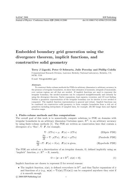
SciDAC 2008Journal of Physics: Conference Series 125 (2008) 012080IOP Publishingdoi:10.1088/1742-6596/125/1/012080(a) Polynomial function of three variables(b) SF Bay digital elevation map dataFigure 1. Domains generated via an implicit functions.• Implicit functions can be used to represent a rich set of geometric shapes (see figure 1)either in functional form or as interpolants of discrete, sampled data (e.g., 2D/3D imagedata [3, 4, 5], digital elevation maps).• Implicit functions can be easily restricted to lower dimensions. This is exploited in thealgorithm that computes moments (see Section 2).• Implicit functions can be extended to arbitrary dimensions allowing computations to bedone in phase spaces or space-time.• Ω can implicitly evolve in time if φ is allowed to change with time, possibly as a functionof other PDE variables or time directly.In this embedded boundary approach, Ω will be discretized on a set of control volumes, V,formed by intersecting rectangular cells with Ω:V = {[ih,(i + e)h] ∩ Ω : i ∈ Z D }, (2)where e ∈ Z D and all its components are one and h is the size of the rectangular cells that are,in this case, square.Given this formulation, the integral of the divergence of the vector field, ∇ · F, over thecontrol volume, V ∈ V, can be transformed by using the divergence theorem into an integralover the boundary of the volume, A = ∂V :∫ ∫∇ · F dV = F · n dA (3)Vwhere n is the normal to A pointing out of V . In control volumes that do not intersect theboundary of Ω, this can be rewritten as A d −: F − · n = −F d − on the low faces and as A d +:F + · n = F d + on the high faces by noting that on the faces the normal points in a coordinatedirection, d. The result is the canonical “(sum of) difference in fluxes (integrated over faces)”formulation of finite volume methods. These methods are as accurate as the approximations tointegrals of F d ± over the faces.2A

SciDAC 2008Journal of Physics: Conference Series 125 (2008) 012080IOP Publishingdoi:10.1088/1742-6596/125/1/012080With these definitions, a finite-volume method for control volumes containing embeddedboundaries can be defined by using the divergence theorem:∫V∇ · F dV =∑± = +,−D∑d=1∫± F± d dA +A d ±∫A EBF · n EB dA, (4)where A d ± = {x : x ∈ V,x d = (i d + 1 2 ± 1 2 )h}, A EB = V ∩ ∂Ω, and n EB = ∇φ/|∇φ|. Note: n EBis defined everywhere in Ω and not simply on ∂Ω. This equation has still not been discretized;that is, it is exact. The integrals over the boundary are discretized by using an P th order Taylorexpansion of F and F d ± about points x EB ∈ A EB and x d ± ∈ A d ± that approximate the centroidsof the domains of integration. In addition, we can expand n EB about some point in the cell(which we take to be the origin of our coordinates), since it is a known smooth function. Usingthese Taylor expansions, we can rewrite equation (4) as follows:∫V∇ · F dV =∑0≤|p|≤P(1 ∑p!± = +,−+ ∇ p F ·∑0≤|r|≤RD∑d=1± (∇ p F d ± ) ∫∇ r n EBr!∫A EBA d ±(x − x d ± )r dA(x − x EB ) p x r dA)+ O(h D+P+R .) (5)Assuming F is discretized on the rectangular grid covered by Ω, one can approximate ∇ p F d ±and ∇ r F to the appropriate order by finite differences. The remaining information required isin the form of moments, namely, integrals of polynomials computed over the V , A d ±, and A EB .Note that x d ± and x EB can also be computed from moments. Computing these is the analogue ofgrid generation for the embedded boundary method. No explicit representation of the irregularboundary is ever needed.2. Moment computationsApproximating the needed moments to the necessary order can be accomplished by taking allmonomials, x p , of a given degree, P, where p is a multi-index and |p| = P, and substitutingF(x) = x p e d into equation (4), where e d is the unit vector in direction d. Note that∂x p /∂x d = p d x p−e dand replacing n EB by its Taylor expansion; then each monomial yieldsthe set of D equations defined byp d∫Vx p−e ddV − n d∫A EBx p dA = ∑± = +,−+ ∑∫±1≤|r|≤RA d ±x p dA(∇ r n dr!∫A EBx (p+r) dA)+ O(h D+P+R ) (6)If the integrals on the LHS are treated as unknowns and the RHS is treated as known, thenthe set of equations formed in this way for all monomials x p where |p| = P forms a systemof linear equations. The number of unknowns is N P −1 + N P (where N P is the number ofmonomials of degree P) and number of equations is DN P . Since N P −1 < N P , if D ≥ 2, this isan overdetermined system and can be solved by least squares. The one-dimensional case can besolved explicitly by using 1D root-finding techniques and integration of monomials (see below).Examining the RHS shows that the first integral is of the same form as the volume integrals onthe LHS except the integral has been restricted to one less dimension and the monomial degree3

SciDAC 2008Journal of Physics: Conference Series 125 (2008) 012080IOP Publishingdoi:10.1088/1742-6596/125/1/012080(a) Borromean (interlocked) rings(b) Gas jet nozzleFigure 2. Domains generated via constructive solid geometry and multiple implicit functions.is one more. Hence, the order of accuracy is the same, ((P + 1) + (D − 1) + R = P + D + R).Using recursion, we can reduce the dimension until D = 1. At this point all the moments canbe computed over A d because A d is the intersection of V with a line parallel to the x d axisand the monomial only has one variable that isn’t constant. The intersection can be found byusing robust 1D root finding algorithms to get the end points of the 1D integral, which is thencomputed explicitly.The second integral on the RHS involves moments over the A EB in the current dimensionbut the degree has increased to P + |r|. Thus, they can be computed recursively. The recursionterminates because as the degree of the monomial moments increases, the dimension and orderof accuracy stays the same. Thus, the value of R (the number of terms in the Taylor series) inthe recursion decreases by |r|. Eventually, there are no terms of the Taylor series on the RHSso this recursion terminates.Overall, the algorithm proceeds by setting up the equations to compute the needed momentsover the needed regions as a least squares problem. Then the RHS is recursively computedrecursing in both dimension and monomial degree. Finally, the original least squares problemsare solved for the unknown moments, and these are used in the flux computations. Since theleast squares problems are always well conditioned and the only computations involving the Ωare the intersections of the Ω with lines parallel to the coordinate axes, this algorithm is veryrobust and straightforward to implement.3. Complex irregular boundariesIn order to construct more complex irregular boundaries, implicit functions can be composed intomore complex implicit functions using constructive solid geometry, CSG. To do so, one mustdefine the complement, intersection, and union of irregular domains, Ω i , defined by implicitfunctions, φ i . To this end we use the following correspondences.Ω complementi⇔ −φ iΩ intersection ⇔ max φ i iΩ union ⇔ min φ i i4

SciDAC 2008Journal of Physics: Conference Series 125 (2008) 012080IOP Publishingdoi:10.1088/1742-6596/125/1/012080Further, coordinate transformations, ψ, of Ω can be implemented asΩ ψ = {x : x ∈ R D , φ(ψ −1 (x)) < 0}.Examples of ψ include rotations, translations, and scaling. In addition to being straightforwardto implement by using implicit functions, CSG is a very robust and intuitive method for buildingcomplex geometry objects and easily manipulating them (see figure 2).Once constructed, only the value of the implicit function representing the irregular domainand its derivatives need to be evaluated in order to compute the necessary moments. This allowsthe embedded boundary method to perform efficiently even on workstations.If good estimates of the bounds of the local Taylor series expansion of the implicit functionsare available, these can be used to dramatically improve performance by subdividing spacerecursively and only evaluating the implicit function where an irregular boundary could exist,i.e., regions where φ(x) could be zero. Thus, the amount of work done is proportional to thenumber of cells containing the irregular boundary and not the entire space. This also allowscells with under resolved geometry to be detected and corrected by adaptively refining thesecells. This has been found to occur routinely when the higher-dimension irregular domains arerestricted to lower dimensions; for example, slices of a well-resolved unit sphere can be circleswith arbitrarily small radii. Once adequate refinement has been done, either the computationcan use the refined computational cells, or they can be coarsened to provide the moments at theoriginal resolution.4. Conclusions and future workIt has been shown that finite volume methods for PDE can be done in arbitrary dimensionto arbitrary accuracy in the presence of irregular boundaries by computing moments, integralsof monomials, over various regions. If the irregular boundary is defined by implicit functions,computing these moments can be computed using the divergence theorem, Taylor expansions,least squares, recursion, and 1D root finding. As a result, an explicit representation of theirregular domain and boundary is never needed nor computed. The resulting computationsare robust and efficient even for complex domains which can be easily defined using implicitfunctions and constructive solid geometry.These methods can be extended to mapped grids by incorporating coordinate mappings in theflux and moment computations. In addition, these methods can be used in any computationalcontext where the algorithm can be reduced to the computation of moments over irregulardomains or boundaries, for example, the integration of functions over these regions.AcknowledgmentThis research was supported by the Office of Advanced Scientific Computing Research of theUS Department of Energy under contract number DE-AC02-05CH11231.References[1] Colella P 2001 Volume-of-fluid methods for partial differential equations Godunov Methods: Theory andApplications E F Toro, 161–177[2] Aftosmis M, Berger M J and Melton J 1998 Robust and efficient Cartesian mesh generation for componentbasedgeometry AIAA J. 36(6) 952–960[3] Deschamps T, Schwartz P, Trebotich D, Colella P, Malladi R and Saloner D 2004 ‘Vessel segmentation andblood flow simulation using level sets and embedded boundary methods (Elsevier International CongressSeries, 1268) 75–80[4] Schwartz P, Adalsteinsson D, Colella P, Arkin, A P and Onsum M 2005 Numerical computation of diffusionon a surface Proc. Nat. Acad. Sci. 102 11151–11156[5] Malladi R, Sethian J A and Vemuri B C, Shape modeling with front propagation: A level set approach IEEETrans. Pattern Anal. Machine Intell. 17:158–175.5