Math 362 Problem Set #9 – Solution 27 April 2012 - Faculty web ...

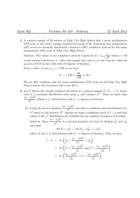
Math 362 Problem Set #9 – Solution 27 April 20121. A random sample of 20 seniors at Edge City High School had a mean mathematicsSAT score of 455 with a sample standard deviation of 69. Assuming that mathematicsSAT scores are normally distributed, construct a 90% confidence interval for the meanmathematics SAT score at Edge City High School.sSolution: The radius of our confidence interval is given by E = t α/2 √ , where s = 69nis the standard deviation, n = 20 is the sample size, and t α/2 is the critical t-value foran area of 0.10 in two tails with 19 degrees of freedom.From a table, we get t α/2 = 1.729, so we haveE = 1.729 × 69 √20≈ 26.7.We are 90% confident that the mean mathematics SAT score for all Edge City HighSchool seniors lies bewtween 428.3 and 481.7.2. Let S denote the sample standard deviation of a random sample Y 1 , Y 2 , . . . , Y n whereeach Y i is normally distributed with mean µ and variance σ 2 . Then we know that(n − 1)S 2follows a χ 2 distribution with n − 1 degrees of freedom.σ 2(a) Using the pivotal quantity(n − 1)S2, describe a confidence-interval estimator forσ 2σ 2 based on the statistic S 2 . Assume we want a confidence level of 1 − α and thattables of the χ 2 distribution are available for any number of degrees of freedom.(n − 1)S2Solution: Since is a pivotal quantity, we start by finding χ 2σ 2L and χ 2 Rsuch thatPr(X < χ 2 L) = Pr(X > χ 2 R) = α/2,where X has a χ 2 distribution with n − 1 degrees of freedom. Then we have)1 − α = Pr(χ 2 (n − 1)S2L < < χ 2σ 2R)= Pr(σ 2 (n − 1)S2< and σ 2 (n − 1)S2>χ 2 Lχ 2 R( )(n − 1)S2= Pr< σ 2 (n − 1)S2< .χ 2 Rχ 2 L

We are 100(1 − α)% confident that σ 2 lies between(n − 1)S2χ 2 Rand(n − 1)S2.χ 2 L(b) A random sample of 20 seniors at Edge City High School had a mean mathematicsSAT score of 455 with a sample standard deviation of 69. Assuming thatmathematics SAT scores are normally distributed, construct a 90% confidenceinterval for the standard deviation of all mathematics SAT scores at Edge CityHigh School.Solution: We first find χ 2 L and χ 2 R so thatPr(X < χ 2 L) = Pr(X > χ 2 R) = 0.05with 19 degrees of freedom. Our χ 2 table says that χ 2 L = 10.117 and χ 2 R = 30.144.The left end of our confidence interval for σ 2 19 × 692is ≈ 3000.90 and the right30.14419 × 692end is ≈ 8941.29. To get a confidence interval for the standard deviation10.117σ, we just take square roots.We are 90% confident that the standard deviation for all mathematics SAT scoresat ECHS lies between 54.78 and 94.56.3. The following data are from a normal distribution with mean µ and variance σ 2 :52.2, 46.4, 34.3, 43.8, 33.6, 32.5.Construct 95% confidence interval estimates for µ and σ.Solution: We find that the sample mean is about 40.46667 and the sample standarddeviation is about 8.156388.The sample size is 6, so our critical t-value has 5 degrees of freedom and an area of0.05 in two tails. We get t α/2 = 2.571, so the radius of our confidence interval for µ isE ≈ 2.571 × 8.156388 √6≈ 8.561.We are 95% confident that µ lies between 49.03 and 31.91.To construct a confidence interval for σ 2 , we find χ 2 L and χ 2 R so that P (X < χ 2 L) =P (X > χ 2 R) = 0.025 with 5 degrees of freedom. In the table, we find χ 2 L = 0.831 andχ 2 R = 12.833. Using the result from problem 2a, we get5 × (8.15639) 212.833≈ 25.9202 and 5 × (8.15639)20.831≈ 400.281

as the left and right endpoints of a 95% confidence interval for σ 2 . To find a confidenceinterval for σ, we take square roots.We are 95% confident that σ lies between 5.09 and 20.01.4. The probability density function for the Student t distribution with ν degrees of freedomis given by[ (Γν+1) ] ( ) −ν+12f T (t) = √ (πν Γν1 +2)t2 2.νFor a fixed ν, the quantity in brackets is a constant, and so the “core” of the distribution) −ν+1is the function t ↦→(1 + t2 2.ν(The quantity in brackets is there in order to make the PDF integrate to 1.)Show that, as ν → ∞, the core of the Student t distribution PDF approaches the coreof the standard normal PDF.What does this tell you about the Student t distribution?Γ ( )ν+12What does it tell you about lim √ (ν→∞ πν Γν2)?( ) −ν+1We need to evaluate lim 1 + t2 2, which we could write asν→∞ νlimν→∞[(1 + t2ν) ν )] −1(1 + t2 2.νUsing continuity and the fact that the limit of the product is the product of the limits,we getlimν→∞) ν+1(1 + t2 2ν==[limν→∞) ν ] −1(1 [ ( )]+ t2 2 −1lim 1 + t2 2νν→∞ ν[e t2] − 1 2· [1] − 1 2= e − t2 2 ,which is the core of the probability density function for the standard normal distribution.

For large values of ν, the Student t distribution is approximately the same as thestandard normal distribution.Furthermore, since the normalizing constants have to match up, we have shown indirectlythatΓ ( )ν+121√ (πν Γν= √ .2)2πlimν→∞5. We showed in a previous problem set that the mean of n independent exponential(1)random variables has a Gamma distribution with parameters r = n and λ = n.(a) Show that the moment-generating function for a random variable Y with a Gammadistribution with parameters r and λ is given by(m Y (t) = 1 −λ) t −r.Solution: We haveE(e tY ) = λrΓ(r)= λrΓ(r)∫ ∞0∫ ∞0e ty y r−1 e −λy dyy r−1 e −(λ−t)y dyAs long as λ − t > 0, this integral converges. In fact, since y r−1 e −(λ−t)y is the“core” of the probability density function for a Gamma distribution, we knowthatIt follows thatas required.∫ ∞0y r−1 e −(λ−t)y dy =Γ(r)(λ − t) r .m Y (t) = λrΓ(r) · Γ(r)(λ − t)( ) rr λ=λ − t(= 1 − t ) −rλ

(b) Now suppose Y follows a Gamma distribution with parameters r = n and λ = n.Let U = √ n(Y − 1), and find the limit of m U (t) as n → ∞.What does this tell you about the mean of a large number of exponential(1)random variables?(m Y −1 (t) = e −t m Y (t) = e −t 1 − t ) −nnand so(m U (t) = e −t√ n1 − √ t ) −n= n(e t √ n(1 − t √ n)) −n.We’ll rewrite this limit in terms of a new variable s =s → 0, so our limit becomeslims→0 (es (1 − s))) − t2s 2 =[]lims→0 (es (1 − s)) 1 −t 2s 2 .t √ n. As n → ∞, we haveThe limit inside the brackets has the form 1 ∞ , and we can attack it using l’Hôpital’srule. We getThus lim(e s (1 − s)) 1s 2 = e − 1 2 ands→0ln lim(e s (1 − s)) 1 ln(e s (1 − s))s 2 = lims→0 s→0 s 2lim m U(t) = limn→∞s→0[e s (1 − s) − e s= lims→0 2se s (1 − s)= lims→0= − 1 2 .−12(1 − s)lims→0 (es (1 − s)) 1s 2 ] −t 2= e t2 2which is the moment generating function for the standard normal random variable.This says that for large n, √ n(Y − 1) has approximately the standard normaldistribution. Working backward, we can conclude that the distribution of Y − 1is approximately normal with mean zero and variance 1 , and so Y , the samplen

mean of our exponential(1) random variables, is approximately normal with mean1 and variance 1 n .That is, if Y 1 , Y 2 , . . . , Y n are independent random variables, each with an exp(1)distribution, then their mean, Y , follows a distribution that is approximatelynormal with mean 1 and variance 1 n .