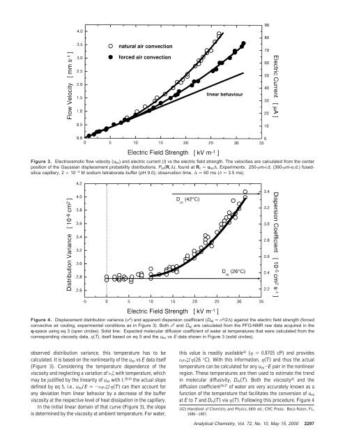
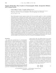
Figure 3. Electroosmotic flow velocity (u eo) and electric current (I) vs the electric field strength. The velocities are calculated from the centerposition of the Gaussian displacement probability distributions, P av(R,∆), found at R c ) u eo∆. Experiments: 250-µm-i.d. (360-µm-o.d.) fusedsilicacapillary, 2 × 10 -3 M sodium tetraborate buffer (pH 9.0); observation time, ∆ ) 60 ms (δ ) 3.5 ms).Figure 4. Displacement distribution variance (σ 2 ) and apparent dispersion coefficient (D ap ) σ 2 /2∆) against the electric field strength (forcedconvective air cooling, experimental conditions as in Figure 3). Both σ 2 and D ap are calculated from the PFG-<strong>NMR</strong> raw data acquired in theq-space using eq 3 (open circles). Solid line: Expected molecular diffusion coefficient of water at temperatures that were calculated from thecorresponding viscosity data, η(T), itself based on eq 5 and the u eo vs E data shown in Figure 3 (solid circles).observed distribution variance, this temperature has to becalculated. It is based on the nonlinearity of the u eo vs E data itself(Figure 3). Considering the temperature dependence of theviscosity and neglecting a variation of ɛ r ζ with temperature, whichmay be justified by the linearity of u eo with I, 39,40 the actual slopedefined by eq 5, i.e., u eo /E )-ɛ 0 ɛ r ζ/η(T) can then account forany deviation from linear behavior by a decrease of the bufferviscosity at the respective level of heat dissipation in the capillary.In the initial linear domain of that curve (Figure 3), the slopeis determined by the viscosity at ambient temperature. For water,this value is readily available 42 (η ) 0.8705 cP) and providesɛ 0 ɛ r ζ/η(26 °C). With this information, η(T) and thus the actualtemperature can be calculated for any u eo -E pair in the nonlinearregion. These temperatures are then used to estimate the trendin molecular diffusivity, D m (T). Both the viscosity 42 and thediffusion coefficient 36,37 of water are very accurately known as afunction of the temperature that facilitates the conversion of u eoat E to T and D m (T) via η(T). Following this procedure, Figure 4(42) Handbook of Chemistry and Physics, 66th ed.; CRC Press: Boca Raton, FL,1986-1987.Analytical Chemistry, Vol. 72, No. 10, May 15, 2000 2297
shows the expected increase of the molecular diffusion coefficientof water (solid line) in comparison with the experimental data.Calculated temperatures cover a range from 26 to 42 °C; i.e., wefind a temperature increase of ∼16 °C above ambient at thehighest power level in the capillary (which is EI ) 2.42 W/m atE ) 31.4 kV/m and I ) 77 µA; Figure 3). The striking feature isthat the measured distribution variance and the apparent dispersioncoefficient can be well accounted for by the temperaturedependence of the molecular diffusivity, and there is no need topropose any contribution of a laminar flow component or effectof a radial temperature gradient in the capillary lumen (at leastwithin the moderate temperature range encountered here). In fact,the experimental data presented in Figures 3 and 4 suggest a plugflowprofile for electroosmosis with axial dispersion only due tomolecular diffusion (as implied by eqs 8 and 9). The results agreewith Raman spectroscopic measurements of temperature gradientsin operating CE capillaries. 43 Those studies have shown that, ifthe average operating temperature is not 25 °C or more aboveambient, radial gradients are small enough that the associatedTaylor dispersion can be neglected.A similar conclusion about the temperature effects in CE wasreached by Knox and McCormack, 39 who showed that theincreased value of the diffusion coefficient (at the actual buffertemperature) can largely explain the reduced number of theoreticalplates obtained for a given separation. They pointed out thatthe differences still observed at higher linear velocities are partlydue to an extra column dispersion caused by injection and detectioneffects. 44,45 Clearly, these factors are absent in the presentPFG-<strong>NMR</strong> study in which the fluid flow field with any (intrinsic)source of dispersion is measured directly, i.e., without introducinga tracer. In this respect, our approach is similar to that of Paul etal., 46 who recently used fluorescence imaging of a photoactivatablerhodamine dye to demonstrate a pure electrokinetic flow behaviorin a 75-µm-i.d. fused-silica capillary (within the resolution of thetechnique). Images collected at a series of time delays after theuncaging event indicate a pluglike velocity profile, and peak widthswere found to have increased only by axial diffusion of the tracer.The caged fluorescent dye is uniformly seeded throughout theactive fluid phase (perfectly mixed) and can be activated at anyposition in the system. Thus, the injection of a dye, a process thatmay affect the initial conditions and dispersion characteristics, 47is circumvented.Starting with the situation in Figure 2 (∆ ) 14.2 ms), it is nowinstructive to follow the time evolution of either displacementdistribution and see the interplay between axial convection andradial diffusion. The (Gaussian) electroosmotic displacementprofiles shown in Figure 5a reveal a constant diffusion coefficient,i.e., D ap ≡ D m (28 °C) ) 2.47 × 10 -5 cm 2 /s at 15.1 kV/m (cf.Figure 4), and the increase in distribution variance scales exactlywith the increase in observation time (eq 9). As demonstrated inFigure 5b, the assumption of a perfect Gaussian shape isreasonable and hardly any symmetric deviation (indicative of aFigure 5. (a) Electroosmotic displacement profiles as a function ofthe observation time (∆ as indicated). E ) 15.1 kV/m, I ) 29 µA(u eo ) 1.34 mm/s). Mobile phase: 2 × 10 -3 M sodium tetraboratebuffer (pH 9.0); 0.7 m × 250 µm i.d. (360 µm o.d.) fused-silicacapillary. (b) P av(R,∆) at∆ ) 90 ms and best Gaussian fit (centerposition, R c ) u eo∆ ) 121 µm).laminar flow component) can be resolved by statistical analysis. 35These observations again indicate a very narrow (if any) velocitydistribution over the whole column cross section (on the inherenttime scale of the measurements), with diffusional broadening atthe actual buffer temperature only.In contrast to the already constant electroosmotic displacementpattern, the influence of radial diffusion in the regime (2D m ∆) 1/2, r c under now laminar flow conditions manifests itself in anexchange between the involved velocity extremes (cf. Figure 2).The Lagrangian correlation length of this flow velocity field ismuch higher than for an ideal EOF profile, and exchange by radialdiffusion proceeds over the whole capillary radius (125 µm), i.e.,on the time scale of a few seconds. Because the velocity gradientchanges with radial position, rather unique axial displacementprofiles are observed at increasing observation times (Figure6). 35,48 In the region of steep velocity gradients near the capillarysurface, for example, an inward diffusion leads to a bump at therear which then grows to consume the former boxcar shape. Dueto the fact that the velocity varies only quadratically with distancefrom the capillary axis (eq 6), the leading edge of the boxcarsubstantially retains its shape in this early stage. Finally, however,the central front also will lose its sharpness and the displacement(43) Liu, K.-L. K.; Davis, K. L.; Morris, M. D. Anal. Chem. 1994, 66, 3744-3750.(44) Sternberg, J. C. Adv. Chromatogr. 1966, 2, 205-270.(45) Huang, X.; Coleman, W. F.; Zare, R. N. J. Chromatogr. 1989, 480, 95-110.(46) Paul, P. H.; Garguilo, M. G.; Rakestraw, D. J. Anal. Chem. 1998, 70, 2459-2467.(47) Tsuda, T.; Ikedo, M.; Jones, G.; Dadoo, R.; Zare, R. N. J. Chromatogr. 1993,632, 201-207. (48) Shankar, A.; Lenhoff, A. M. AIChE J. 1989, 35, 2048-2052.2298 Analytical Chemistry, Vol. 72, No. 10, May 15, 2000