Gravimetric Geoid Determination in the Andes - ResearchGate

employ the 2D-FFT spherical Stokes convolution toevaluate the kernel function (Strang Van Hess,1990).R∆ϕ∆λ−1N g = F {F( ∆g cos ϕ)F(∆ϕ,∆λ,ϕ m ))} (3)∆4πγwhere N ∆g are the estimated residual gravimetricgeoid heights or residual cogeoid heights.The indirect effect on the geoid is∆= Tγh ρ(x,y, z)(h P − z)c =− Gdxdydz (10)Ph PN ind (4) r3( x P − x, y P − y, h P − z)where ∆T is the change of the potential at the geoiddue to the terrain reduction applied and γ is thenormal gravity. The indirect effect on gravity, whichreduces gravity anomalies from the geoid to thecogeoid should be added to Eq. 1 for Helmert’ssecond method of condensation and Airy method,and can be expressed by (Heiskanen and Moritz,1967) byδ∆g=0.3086N ind [mGal] (5)where δ∆g is the indirect effect on gravity given by(Sideris and She, 1995) asδ∆g2πGρh=γ∫∫∫E2(9)and c P is the classical terrain correction given by thefollowing equation:where ρ(x,y,z) is the topographical density at therunning point and G is the gravitational constant.The indirect effect on the geoid, up the secondorder is in planar approximation (Wichiencharoen,1982)23 3πGρhP Gρh − hN = − −Pindγ γ ∫∫dxdy (11)36 rwhere r 0 is the planar distance between computationpoint and data point.E0The RTM method estimates the quasigeoid. Thefree-air gravity anomalies and Eq. 1 refer to thesurface of the topography. Eq. 2 for height anomalyor quasigeoid determination can be formulated asζ = ζ + ζ ∆ + ζ(6)GMgindwhere ζ ind represents the indirect effect on thequasigeoid for the RTM reduction.In order to compare the results of this methodwith the other three reduction methods and to makecomparisons with the GPS/leveling derived geoid,the quasigeoid in the RTM method is converted togeoid using the quasigeoid-geoid separation given in(Heiskanen and Moritz, 1967) as∆gBN ≈ ζ + H(7)γwhere γ and ∆g B represent the mean normal gravityand Bouguer anomaly, respectively.2.1 Helmert’s second method of condensationHelmert’s second method of condensation condensesthe topographic masses on a surface layer on thegeoid and it can be view as a limiting case of Pratt-Hayford when the depth of condensation goes tozero. Before applying Stokes’s formula, the indirecteffect on gravity has been considered.The terrain effect on gravity ∆g T is given by2.2 Rudzki inversion methodThe Rudzki inversion method is a reduction wherethe indirect effect is zero. Rudzki shifts all thetopographic masses inside the geoid.∆g T =A T – A inv (12)where A T is the attraction of the topographic masses,A inv is the attraction of the inverted masses, with thedensity of the topographic masses being equal to thedensity of the inverted masses and the thickness ofthe inverted masses is equal to the height of thetopography.AAinvh ρ(x,y,z)(hP− z)= −Gdxdydz (13)03r (x − x, y − y,h z)T ∫∫∫ −Eh P (x, y,z)(h P z)G∫∫∫ − ρ −= −dxdydz (14)−h−h3P r (x − x,y − y,h− z)EPPP3.3 RTM methodThe RTM reduction method takes into account thehigh frequencies of the topography. The effect of thetopography above a long wavelength topographicsurface is first removed and later restored.The RTM gravity terrain effect, ∆g T is given bythe approximate expression (Forsberg, 1984)PPP∆g T = -δ∆g - c P (8)

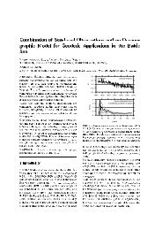
∆ g = ∆g≈ 2πGρ(h− h ) − c (15)TRTMwhere h is the topographic height given by a digitalterrain model, h ref is the height of a smooth meanreference surface and c P is the classical terraincorrection.The RTM geoid effect is expressed in linearapproximation as:∞ ∞ hG (h h ) ∞ ∞Gρ1 ρ − ref 1ζ T = ζ RTM = ∫ ∫ ∫ dxdydz =∫ ∫ dxdyγ −∞−∞ href rγ −∞ −∞ rowhere r 0 is the planar distancerefP(16)2.4 Airy methodThe object of an isostatic reduction of gravity,according to Airy-Heiskanen (AH) model is theregularization of the earth’s crust (see Heiskanen andMoritz, 1967). The terrain effect ∆g T is∆ g = A − A(17)ATTCh ρ(x,y,z)(h P − z)= −Gdxdydz (18)03r (x − x, y − y,h z)T ∫∫∫ −EPPT hP(x, y,z)(h P z)Ac G∫∫∫ − − ∆ρ −= −dxdydz (19)−T−t−h3P r (x − x, y − y,h − z)EPwhere A T is the attraction of the topographic massesabove the geoid and A c is the attraction of thecompensated masses according AH model, t is theroot height, h is the height of the topography, ∆ρ isthe density contrast between the upper mantle andthe crust, ρ is the crust density and T is the thicknessof the Earth’s crust.The change of potential ∆T in equation (4) is forthe isostatic reduction expressed by∆T = T T − T C(20)where T and are the gravitational potentials ofTTCthe topography and compensating massesrespectivelyh ρ(x,y,z)T T = −G∫∫∫ dxdydz (21)0 r (x − x, y − y,h − z)TCEPPT ∆ρ(x, y,z)= −G∫∫∫ − dxdydz (22)−T−tr (x − x, y − y,h − z)EPPPPPPP3 Area under study and data availabilityThe area under study is located in the roughest areaof Argentina, bounded by 20°S to 42°S in latitudeand 67°W to 72°W in longitude.The point gravity measurements, provided bydifferent sources, were referenced to theInternational Standardization Net 1971 (I.G.S.N.71).A total of 11132 measured gravity points, with amean data spacing of approximately 12 km are usedin the mountainous area The distribution of thegravity points is shown in Figure 1. Gravityanomalies are computed using the parameters ofGRS80 according to the formulas given in Torge,1989.The reference gravity field is computed from theEGM96 geopotential model (Lemoine et al., 1998)complete to degree and order 360.The global digital elevation model GTOPO30with a horizontal grid spacing of 30 arc seconds(approximately 1 kilometre) is used to represent thetopography in the test area. A total of 166GPS/leveling points in three different networks wereused for comparison with the gravimetric geoid inthe rough area. The distribution of the GPS pointscan be seen in Figure 2.4 Geoid modeling developmentc PTerrain corrections ( ) were calculated by FFT foreach gravity point from the GTOPO30 DEM usingthe Tc2DFTPL program (Li, 1993). A third orderterm of a mass prism model was used. The indirecteffect on gravity due to Helmert’s second method ofcondensation was considered before applyingStokes’s formula and its computation on the geoidshould be considered to, at least, second order term.The maximum indirect effects are correlated withthe topography. The statistics of the topographic dataand statistics of terrain corrections in gravity stationscan be seen in Table 1.Table 1. Statistics of the GTOPO30. Unit:[m] and c P .Unit:[mGal]Max Min Mean ±σGTOPO30 6795 0 1399 1465c P 42.13 0.20 2.55 2.70The TC program was used to compute the RTMeffects and the topographic-isostatic effects on bothgravity and geoid (Forsberg, 1984) and this programwas modified to compute the Rudzki inversionmethod (Bajracharya et al., 2001). The statistics ofthe gravity anomalies calculated with the fourtopographic gravity reductions are presented inTable 2.

5 ConclusionsFour different gravity reduction methods have beenpresented. They treat the topography in a verydifferent way. Helmert’s second method ofcondensation and the RTM method are the mostused reduction techniques for the determination of agravimetric geoid. In this paper, AH reduction aswell as the Rudzki inversion method were alsoapplied. The last one is not used very often,although it has the advantage of no indirect effects.The gravimetric geoid computed with the Rudzkiinversion method gave better results compared withthe GPS/leveling-derived geoid before and after fitand was the only method that improved thegravimetric geoid compared to the EGM96 results.The gravimetric data needs to be improved in thearea of the Andes in order to see furtherimprovements in the geoid.ReferencesBajracharya, S., Kotsakis C., Sideris M. G., 2001. GeoidDetermination Using Different Gravity ReductionTechniques. Presented in IAG meeting, Budapest.Forsberg, R., 1984. A study of terrain reductions, densityanomalies and geophysical inversion methods in gravityfield modeling. Report No. 355, Department of GeodeticScience and Surveying, The Ohio State University,Colombus, Ohio, USA.GTOPO30,1996.(http://edcdaac.usgs.gov/gtopo30/gtopo30.html)..Heiskanen, W.A. and Moritz, H., 1967. Physical Geodesy.Freeman and Company, San Francisco.Lemoine, F. G., Kenyon, S. C., Factim, J. K., Trimmer, R. G.,Pavlis, N. K., Chinn, D. S., Cox, C. M., Klosko, S. M.,Luthcke, S. B., Torrence, M. H., Wang, Y. M., Williamson,R. G., Pavlis, E. C., Rapp, H. and Olson, T. R., 1998. Thedevelopment of the joint NASA GSFC and the NationalImagery and Mapping Agency (NIMA) GeopotentialModel EGM 96. Pub. Goddard Space Flight Center.Li, Y., 1993. HFTGVBP Software package for the solution ofGVBP by means of fast Hartley/Fourier Transform.TOPOGEOP Software packages to evaluate theTOPOgraphic effects on GEOdetic /GEOPhysicalObservation. Department of Geomatics Engineering, TheUniversity of Calgary.Sideris, M.G., She, B.B., 1995. A new high-resolution geoidfor Canada and part of U.S. by the 1D-FFT method. BullGeod 69, 92-108.Strang van Hees G., (1990). Stokes' formula using fast Fouriertechniques. Manuscripta Geodaetica, Vol. 15, pp. 235-239.Torge, W., 1989. Gravimetry, Walter de Gruyter, Berlin.Wichiencharoen, C., 1982. The indirect effects on thecomputation of geoid undulations. OSU Report. No 336,Department of Geodetic Science and Suveying, The OhioState University, Columbus, Ohio, USA.