Discrete Time Markov Chains, Limiting Distribution and Classification

State classification by f (n)iiClassification of Markov chains◮ A state is recurrent (persistent) if f ii(= ∑ )∞n=1 f (n)ii= 1◮ A state is positive or non-null recurrent if E(Ti ) < ∞.E(T i ) = ∑ ∞ (n)n=1nfii= µ i◮ A state is null recurrent if E(Ti ) = µ i = ∞◮ A state is transient if f ii < 1.In this case we define µ i = ∞ for later convenience.◮ A peridoic state has nonzero p ii (nk) for some k.◮ A state is ergodic if it is positive recurrent and aperiodic.◮ We can identify subclasses of states with the sameproperties◮ All states which can mutually reach each other will be ofthe same type◮ Once again the formal analysis is a little bit heavy, but try tostick to the fundamentals, definitions (concepts) and resultsBo Friis NielsenLimiting Distribution and ClassificationBo Friis NielsenLimiting Distribution and ClassificationProperties of sets of intercommunicating states◮ (a) i and j has the same period◮ (b) i is transient if and only if j is transient◮ (c) i is null persistent (null recurrent) if and only if j is nullpersistentA set C of states is called◮ (a) Closed if p ij = 0 for all i ∈ C, j /∈ C◮ (b) Irreducible if i ↔ j for all i, j ∈ C.TheoremDecomposition Theorem The state space S can be partitioneduniquely asS = T ∪ C 1 ∪ C 2 ∪ . . .where T is the set of transient states, and the C i are irreducibleclosed sets of persistent states□LemmaIf S is finite, then at least one state is persistent(recurrent) andall persistent states are non-null (positive recurrent) □Bo Friis NielsenLimiting Distribution and ClassificationBo Friis NielsenLimiting Distribution and Classification

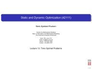
The state probabilitiesLimiting distributionFor an irreducible aperiodic chain, we have that1p (n)ij→ 1 µ jas n → ∞, for all i and j0.90.80.70.60.50.40.30.20.100 10 20 30 40 50 60 70Three important remarks◮ If the chain is transient or null-persistent (null-recurrent)p (n)ij→ 0◮ If the chain is positive recurrent p (n)ij→ 1 µ j◮ The limiting probability of X n = j does not depend on thestarting state X 0 = ip (n)jBo Friis NielsenLimiting Distribution and ClassificationBo Friis NielsenLimiting Distribution and ClassificationThe stationary distributionStationary distribution◮ A distribution that does not change with n◮ The elements of p (n) are all constant◮ The implication of this is p (n) = p (n−1) P = p (n−1) by ourassumption of p (n) being constant◮ Expressed differently π = πPDefinitionThe vector π is called a stationary distribution of the chain if πhas entries (π j : j ∈ S) such that◮ (a) π j ≥ 0 for all j, and ∑ j π j = 1◮ (b) π = πP, which is to say that π j = ∑ i π ip ij for all j.□VERY IMPORTANTAn irreducible chain has a stationary distribution π if and only ifall the states are non-null persistent (positive recurrent);in thiscase, π is the unique stationary distribution and is given byπ i = 1 µ ifor each i ∈ S, where µ i is the mean recurrence time ofi.Bo Friis NielsenLimiting Distribution and ClassificationBo Friis NielsenLimiting Distribution and Classification

The solution of π = πP continued◮ The vector π is a left eigenvector of P.◮ The main theorem says that there is a unique eigenvectorassociated with the eigenvalue 1 of P◮ In practice this means that the we can only solve but anormalising condition◮ But we have the normalising condition by ∑ j π j = 1 thiscan expressed as π1 = 1. Where⎛ ⎞111 = ⎜ ⎟⎝ . ⎠1Roles of the solution to π = πPFor an irreducible Markov chain, (the condition we need toverify)◮ The stationary solution. If p (0) = π then p (n) = π for all n.◮ The limiting distribution, i.e. p (n) → π for n → ∞ (theMarkov chain has to be aperiodic too). Also p (n)ij→ π j .◮ The mean recurrence time for state i is µ i = 1 π i.◮ The mean number of visits in state j between twosuccessive visits to state i is π jπ i.◮ The long run average probability of finding the Markov1∑chain in state i is π i . π i = lim nn→∞ n k=1 p(k) ialso true forperiodic chains.Bo Friis NielsenLimiting Distribution and ClassificationBo Friis NielsenLimiting Distribution and ClassificationExample (null-recurrent) chain⎡P =⎢⎣p 1 p 2 p 3 p 4 p 5 . . .1 0 0 0 0 . . .0 1 0 0 0 . . .0 0 1 0 0 . . .0 0 0 1 0 . . .0 0 0 0 1 . . .. . . . . . . . . . . . . . . . . .For p j > 0 the chain is obviously irreducible.The main theorem tells us that we can investigate directly forπ = πP.π 1 = π 1 p 1 + π 2 π 2 = π 1 p 2 + π 3 π j = π 1 p j + π j+1⎤⎥⎦π 1 = π 1 p 1 + π 2 π 2 = π 1 p 2 + π 3 π j = π 1 p j + π j+1we getπ 2 = (1−p 1 )π 1 π 3 = (1−p 1 −p 2 )π 1 π j = (1−p 1 · · ·−p j−1 )π 1⎛ ⎞∑j−1∑∞π j = (1 − p 1 · · · − p j−1 )π 1 ⇔ π j = π 1⎝1 − p i⎠ ⇔ π j = π 1i=1i=jNormalisation∞∑∞∑ ∑∞ ∑∞ i∑ ∑∞π j = 1 π 1 p i = π 1 p i = π 1 ip ij=1j=1 i=ji=1 j=1i=1p iBo Friis NielsenLimiting Distribution and ClassificationBo Friis NielsenLimiting Distribution and Classification

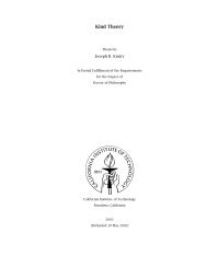
Reversible Markov chainsp 11p121 2p21p22P =[ ]p11 p 12p 21 p 22◮ Solve sequence of linear equations instead of the wholesystem◮ Local balance in probability flow as opposed to globalbalance◮ Nice theoretical constructionBo Friis NielsenLimiting Distribution and ClassificationBo Friis NielsenLimiting Distribution and ClassificationLocal balance equationsπ i = ∑ jπ j p jiTerm for term we getπ i · 1 = ∑ jπ j p ji∑π i p ij = ∑jjπ i p ij = π j p jiπ j p ji∑π i p ij = ∑jjπ j p jiIf they are fulfilled for each i and j, the global balance equationscan be obtained by summation.Bo Friis NielsenLimiting Distribution and ClassificationBo Friis NielsenLimiting Distribution and Classification

Why reversible?Another look at a similar questionP{X n−1 = i ∩ X n = j} = P{X n−1 = i}P{X n = j|X n−1 = i}and for a stationary chain= P{X n−1 = i}p ijπ i p ijFor a reversible chain (local balance) this is π i p ij = π j p ji =P{X n−1 = j}P{X n = i|X n−1 = j} = P{X n−1 = j ∩ X n = i} thereversed sequence.P{X n−1 = j|X n = i} = P{X n−1 = j ∩ X n = i}P{X n = i}= P{X n−1 = j}P{X n = i|X n−1 = j}P{X n = i}For a stationary chain we getπ j p jiπ i= P{X n−1 = j}p jiP{X n = i}The chain is reversible if P{X n−1 = j|X n = i} = p ij leading tothe local balance equationsp ij = π jp jiπ iBo Friis NielsenLimiting Distribution and ClassificationBo Friis NielsenLimiting Distribution and ClassificationExercise 10 (16/12/91 ex.1)In connection with an examination of the reliability of somesoftware intended for use in control of modern ferries one isinterested in examining a stochastic model of the use of acontrol program.The control program works as " state machine " i.e. it can be ina number of different levels, 4 are considered here. The levelsdepend on the physical state of the ferry. With every shift oftime unit while the program is run, the program will change fromlevel j to level k with probability p jk .Two possibilities are considered:The program has no errors and will run continously shifting between the fourlevels.The program has a critical error. In this case it is possible that the error isfound, this happens with probality q i , i = 1, 2, 3, 4 depending on the level.The error will be corrected immediately and the program will from then on bewithout faults.Alternatively the program can stop with a critical error (the ferry will continueto sail, but without control). This happens with probability r i , i = 1, 2, 3, 4.In general q i + r i < 1, a program with errors can thus work and the error isnot nescesarily discovered. It is assumed that detection of an error, as wellas the apperance of a fault happens coincidently with shift between levels.The program starts running in level 1, and it is known that the programcontains one critical error.Bo Friis NielsenLimiting Distribution and ClassificationBo Friis NielsenLimiting Distribution and Classification

Solution: Question 1Question 1 - continuedFormulate a stochastic process ( Markov chain) in discretetime describing this system.The model is a discrete time Markov chain. A possibledefinition of states could be0: The programme has stopped.1-4: The programme is operating safely in level i.5-8: The programme is operating in level i-4, the criticalerror is not detected.The transition matrix A is⎡A = ⎣1 ⃗ 0 ⃗ 0⃗ 0 P 0⃗r Diag(q i )P Diag(S i )P⎤⎦⃗r =The model is a discrete time Markov chain. Where P = {p ij }⎡⎢⎣⎤r 1r 2r 3r 4⎥⎦ Diag(S i ) =⎡⎢⎣Diag(q i ) =⎤S 1 0 0 00 S 2 0 0⎥0 0 S 3 0 ⎦0 0 0 S 4⎡⎢⎣⎤q 1 0 0 00 q 2 0 0⎥0 0 q 3 0 ⎦0 0 0 q 4S i = 1 − r i − q iBo Friis NielsenLimiting Distribution and ClassificationBo Friis NielsenLimiting Distribution and ClassificationQuestion 1 - continuedSolution question 2⎡A =⎢⎣Or without matrix notation:⎤1 0 0 0 0 0 0 0 00 p 11 p 12 p 13 p 14 0 0 0 00 p 21 p 22 p 23 p 24 0 0 0 00 p 31 p 32 p 33 p 34 0 0 0 00 p 41 p 42 p 43 p 44 0 0 0 0r 1 q 1 p 11 q 1 p 12 q 1 p 13 q 1 p 14 S 1 p 11 S 1 p 12 S 1 p 13 S 1 p 14r 2 q 2 p 21 q 2 p 22 q 2 p 23 q 2 p 24 S 2 p 21 S 2 p 22 S 2 p 23 S 2 p 24 ⎥r 3 q 3 p 31 q 3 p 32 q 3 p 33 q 3 p 34 S 3 p 31 S 3 p 32 S 3 p 33 S 3 p ⎦ 34r 4 q 4 p 41 q 4 p 42 q 4 p 43 q 4 p 44 S 4 p 41 S 4 p 42 S 4 p 43 S 4 p 44Characterise the states in the Markov chain.With reasonable assumptions on P (i.e. irreducible) we getState 0 Absorbing1 Positive recurrent2 Positive recurrent3 Positive recurrent4 Positive recurrent5 Transient6 Transient7 Transient8 TransientBo Friis NielsenLimiting Distribution and ClassificationBo Friis NielsenLimiting Distribution and Classification

Solution question 3We now consider the case where the stability of the system hasbeen assured, i.e. the error has been found and corrected, andthe program has been running for long time without errors. Theparameters are as follows.P i,i+1 = 0.6 i = 1, 2, 3 P i,i−1 = 0.2 i = 2, 3, 4P i,j = 0 |i − j| > 1 q i = 10 −3i r i = 10 −3i−5Characterise the stochastic proces, that describes thestable system.The system becomes stable by reaching one of the states 1-4.The process is ergodic from then on. The procces is areversible ergodic Markov chain in discrete time.Solution question 4For what fraction of time will the system be in level 1.We obtain the following steady state equationsπ i = 3 i−1 π 14∑3 i−1 π 1 = 1 ⇔ 40π 1 = 1i=1π 1 = 140The sum ∑ 4i=1 3i−1 can be obtained by using∑ 4i=1 3i−1 = 1−341−3 = 40.4∑i=13 i−1 π 1 = 1 ⇔ 1 − 341 − 3 π 1 = 1Bo Friis NielsenLimiting Distribution and ClassificationBo Friis NielsenLimiting Distribution and Classification