Lab01 - Web Physics - IUPUI

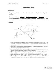
IUPUI Physics Department218/P201 LaboratoryI. IntroductionMeasurement: The BasicsPhysics is first and foremost an experimental science, meaning that its accumulatedbody of knowledge is due to the meticulous experiments performed by teams ofresearchers throughout the world. These experiments yield measurements that givephysicists a peek into the inner workings of nature. The data is then analyzed in anattempt to uncover subtle relationships between various measured quantities such aslength, time, mass, force, voltage, etc. Mathematics is used at every step of theexperimental process, from the initial design phase to the final analysis of the data. Youcannot begin to fully understand nor appreciate the central role of experimentation inphysics unless you are introduced to the mathematics typically used in a physicslaboratory. You also need to familiarize yourself with lab terminology and a few basictechniques before you perform your first physics experiment.In this lab you will learn how towrite measurements correctly, briefly, and clearly, using significant figuresand error notation.determine the number of significant figures in any experimental result.distinguish between random and systematic errors and how they affect theaccuracy and precision of your data.plot your data properly and draw the best-fit line.II. Significant FiguresExperiments are never perfect; there is no such thing as an exact measurement. Inother words, measurements always have uncertainties that reflect the inherent limitationsof the experiment. Because of these obvious though important facts, we must take extracare in the way we record our data. For example, suppose you measure the thickness ofyour textbook with an ordinary ruler and get 4.2 cm. Your result is said to be reliable tothe nearest millimeter (0.1 cm); any digits smaller than 1 mm are uncertain simplybecause you were unable to measure them. It is inappropriate to record yourmeasurement as 4.20 cm or 4.200 cm or 4.2000...cm (with an infinite number of trailingzeroes) because you did not measure those additional digits. In fact, you could write yourmeasurement as 4.2????.. cm, where the question marks remind us that those digits areuncertain.Now suppose you used a Vernier caliper instead of a ruler and measured the thicknessto be 4.235 cm. This new measurement is more reliable since the Vernier calipermeasures to the nearest 0.01 mm (0.001 cm) and has less uncertainty than your previousvalue. Nevertheless, there are still digits lower than 0.01 mm that have not beenmeasured: 4.235????... cm. It should be abundantly clear at this point that there is noway to avoid the presence of uncertain digits in any measured number. We mustconstantly be mindful of this limitation whenever we record data directly from ourmeasuring devices and also whenever we use our data in formulas. A quick and easyway to identify digits that are certain or uncertain is through significant figures.Page 1 of 8

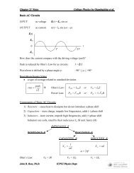
IUPUI Physics Department218/P201 LaboratoryA digit is a significant figure if it is(a) any nonzero number;(b) a trailing zero after the decimal point;(c) any zero between two significant digits.Examples:3.00 3 sig figs 1.0070 5 sig figs800 1 sig fig 800.0 4 sig figs3.24×10 -5 3 sig figs 0.00324 3 sig figsIII. Calculations with Significant FiguresSuppose we add 1.29 and 4.5. If these are “perfect” numbers, then their sum isobviously 5.79. But, if these numbers are measured, then we need to take into accounttheir uncertainties in order to properly compute the sum:1.29???...+ 4.5???? ...But how is it possible to add certain digits to uncertain digits such as 9 + ? in the thirdcolumn? We need to use the following rule:Whenever you add or subtract experimental numbers, the result shouldhave the greatest uncertainty (i.e. fewest digits to the right of thedecimal).In the above example, our final answer must be rounded to the nearest 0.1 since 4.5has the greater uncertainty. Our answer is 5.8.Other arithmetic operations also have special rules to keep the uncertainties in check:Examples:Whenever you multiply or divide experimental numbers, the resultshould have the least number of significant figures.Whenever you raise an experimental number to a power or root, theresult should have the same number of significant figures.123,400 ÷ 5 = 20,000 (1 sig fig)144 .0 = 12.00 (4 sig figs)2π(6.60 × 10 -15 ) = 4.14 × 10 -14 (3 sig figs)Note in the last example that 2 and π are perfect numbers, which have no uncertainty!This is true for all integers, rational numbers, and special mathematical constants thatappear in physics formulas (-5, ¾, e, 2 , etc.)Page 2 of 8

IUPUI Physics Department218/P201 LaboratoryIV. Errors, Precision, and AccuracyThe term error is a synonym for the uncertainty that is present in every measurement.Experimental errors are not mistakes – mistakes can be avoided, errors cannot. There aretwo principal types of errors: Random errors cause random variations in repeated measurements. Eachmeasurement is different by a different amount: some are bigger, some are smaller.Random errors are minimized by taking many measurements and computing the average.The average value is regarded as the value that best represents the data, because thefluctuations tend to cancel each other out when you sum the individual measurements. Systematic errors shift each measurement by the same amount in the samedirection. Unlike random errors, we cannot minimize systematic errors by simplyrepeating the experiment many times. Instead we must make sure that our equipment isproperly calibrated and that other experimental controls are in place before we begincollecting data.There are two other terms that are closely associated with errors:The precision of a set of measurements is inversely related to the size of therandom error. Data that is very precise “clusters” tightly together, indicatingsmall random error.The accuracy of a set of measurements is inversely related to the size of thesystematic error. Data that is very accurate is centered around an acceptedstandard value, indicating small systematic error.A dartboard best illustrates the difference between precision and accuracy:HIGH PRECISION HIGH PRECISION LOW PRECISION LOW PRECISIONHIGH ACCURACY LOW ACCURACY HIGH ACCURACY LOW ACCURACYV. Calculating Errors and DiscrepanciesWhenever experimental results are presented in a lab report or in a scientific paper,all sources of error must be also reported and their effects explained in detail. Simplyusing the rules of significant figures is far too crude a method to express and containerrors in measurements. A better method involves explicitly recording the size of theerror along with your measurement. The general format is( x x) unitswhere x is your best measurement (or the average value if you have more than onemeasurement) and x is its absolute error.Page 3 of 8

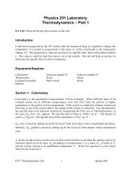
IUPUI Physics Department218/P201 LaboratoryExample: (9.8 ± 0.2) m/s 2In the above example, 9.8 m/s 2 is the average value and 0.2 m/s 2 is the error. The ±indicates that the measurements range between 9.6 m/s 2 and 10.0 m/s 2 .The fractional (or relative error) and the percent error are alternative ways ofexpressing the error:xfractional error = xpercent error = (fractional error)×100%Example: For the previous example, the fractional error is 0.20/9.8 = 0.020 and thepercent error is 2.0%. You could express the result as 9.8 m/s 2 ± 2.0%.It is often a matter of taste or expediency whether you choose to record your errors inabsolute, fractional, or percent form.When an experimental result is compared with a more reliable result (such as a resultaccepted by the international scientific community), the difference between the two iscalled the discrepancy, which can also be expressed in absolute, fractional, or percentform:absolute discrepancy = | A E |fractional discrepancy =A Epercent discrepancy = (fractional disc)×100%Awhere A is the accepted result, E is the experimental result, and the bars | * | indicateabsolute value (discrepancies are always positive).The following criterion is used to judge the accuracy of your results:Example:An experimental result agrees with an accepted value only if thediscrepancy between the two values is numerically less than the error inthe result. If this is case, we conclude that the result is accurate.Suppose you perform an experiment to measure the speed of sound in air (at STP).Your final result is 342 ± 1 m/s. The accepted value is 344 m/s. The absolutediscrepancy is |344 – 342| = 2 m/s which is greater than the absolute error (1 m/s). Yourresult does not agree with the accepted value and, therefore, is inaccurate.VI. Graphing and Linear InterpolationA graph is an accurate two-dimensional representation of experimental data. If youplot a graph by hand, use only high-quality graph paper (which you can purchase at thePage 4 of 8

IUPUI Physics Department218/P201 LaboratoryJAG Bookstore.) Cheaper graph paper often has slightly distorted gridlines that willaffect the accuracy of your plot.Every hand-drawn graph must conform to certain specifications:1) Choose scales (tick marks) on your horizontal and vertical axes such that your datapoints are spread across the entire sheet.2) Draw your axes with a sharp pencil. Label each axis and your tick marks. Recordthe units.3) Use a sharp pencil to plot your points. Pens are acceptable but their marks cannotbe erased.4) Do not connect the dots with line segments! Instead, fit your data to a singlestraight line or a curve.5) Include a brief title at the top that clearly describes what has been plotted.In this introductory lab, you will only deal with data that follows a straight line. Asyou know, the equation of a line in the xy plane is given by y = mx+b, where m is theslope and b is the y-intercept (y = b when x = 0). To graph our experimental data weneed to decide which quantity is the independent variable (x) and which is the dependentvariable (y). If our measurements come with absolute errors, we need to include them aserror bars in graph.Think of an error bar as an interval along the x axis or the y axis. For example, in PartV we considered the measurement (9.8 ± 0.2) m/s 2 . The error bar represents the interval9.6 m/s 2 x 10.0 m/s 2 :[----------o----------]9.6 9.8 10.0Once we have plotted our pairs of points (x, y) along with their respective error bars, thenwe can draw the best-fit line through our data.The best-fit line is that line that passes through the “middle” of the data. If you areplotting by hand, then it is wise to use a clear plastic ruler when you plot your best-lineline. Position the ruler so that there are approximately an equal number of points on eachside of your straightedge. Of course, you would like all the points to line up along thestraightedge. Since that rarely if ever occurs, you try to “split the difference” by finding abalance. When you have found the middle, scribe your line.To determine the slope of the best-fit line, pick two points (x 1 , y 1 ) and (x 2 , y 2 ) alongthe line and use the standard formulam =yx22 y1 x1You are frequently asked the calculate the slope of the best-fit because it has aphysical interpretation.Note to Excel users: If you wish to plot the best-fit line and compute its slope, clickon your graph. Now go to the Chart menu and select Add Trendline. Under Type, clickPage 5 of 8

IUPUI Physics Department218/P201 Laboratoryon Linear; under Options, check Display equation on chart. You should see your best-fitline and its equation in the form y = mx+b.Example:x [s] 1.0 0.4 2.0 0.3 3.0 0.3y [m/s] 3.1 0.5 5.5 0.9 6.4 0.5y(m/s)x=3.0, y=6.4+0.5d (5.5, 9.5)-0.5slope = (9.5-4)/(5.5-1.5)2= 5.5/4=1.3m/ sc (1.5, 4)x(s)Figure 1. Graph of velocity vs. time. The slope represents acceleration.F=(m2-m1)g (N)0.60.50.40.30.20.10y = 0.5708x - 0.00650 0.2 0.4 0.6 0.8 1a (m/s2)Figure 2. Graph of net force vs. acceleration.Page 6 of 8

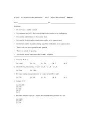
IUPUI Physics Department218/P201 LaboratoryMeasurement WorksheetWrite the number of significant figures in each number.1) 0.150 4) 63.0002) – 490 5) 0.75 ×10 83) 63,000 6) 00.001Round the number 19.9605 to the specified number of significant figures.7) 4 sig figs 9) 2 sig figs8) 3 sig figs 10) 1 sig figPerform the following calculations. Round your final answers according to the rules forsignificant figures (see Part III).611) 12.00 – 0.0462 13) (9.0 10 )12)(8.0)(1.50)4.22214) ½ (9.80)(0.5) 2Use a ruler to measure the length of each line segment. Estimate the absolute error inyour measurement. Express your answer in the form ( x x) cm.15) |------------------------|16) |-------------------------------|17) |------------------------------------------------------|18) Describe at least three experimental errors in measuring the length of the linesegments.19) Describe at least three ways to improve the accuracy of your measurements.Page 7 of 8

IUPUI Physics Department218/P201 Laboratory20) Explain how a wristwatch could be simultaneously very precise yet very inaccurate.(This is not a trick question!)21) The following are measurements of the density of pure gold in g/cm 3 :19.0, 21.1, 20.8, 19.7, 19.9, 20.8, 20.6, 20.0, 20.7, 19.8(a) Calculate the average density.(b) Calculate the absolute error if each density is ±2%.(c) Does your result in Part (a) agree with the accepted value of 19.3? Explain.22)x 1.5 2.3 3.7 4.2 5.3 6.9 7.8y 6.6 9.4 14.8 16.4 20.8 26.3 29.9(a) Graph the above data either by hand or using Excel.Remember the graph specifications listed in Part VI?(b) Draw error bars at each point. (Assume ±10% for each point.)(c) Draw the best-fit line and determine its slope and y-intercept.slope m =y-intercept b =Page 8 of 8