The Hierarchically Tiled Arrays Programming Approach

More documents

Recommendations

Info

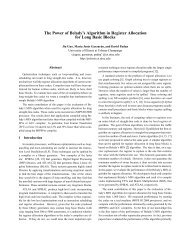
a = hta(MX,{dist}, [P 1]);b = hta(P, 1, [P 1]);b{:} = V;r = a * b;Figure 4: Sparse matrix vector product.for i = 1:nc = c + a * b;a = circshift(a, [0, -1]);b = circshift(b, [-1, 0]);endWhile the previous example only required communicationbetween the client, which executes the main thread, andeach individual server, Cannon’s matrix multiplication algorithm[4] is an example of code that also requires communicationbetween the servers.The algorithm has O(n) time complexity and uses O(n 2 )processors (servers). In our implementation of the algorithm,the operands, denoted a and b respectively, areHTAs tiled in two dimensions which are mapped onto amesh of n × n processors.Figure 5: Main loop in Cannon’s algorithm.6 ×6 matrix is distributed on a 2 ×2 mesh of processors asthe the last parameter of the HTA constructor indicates.In the future we plan to offer more mappings and a representationfor hierarchical organizations of processors.3. PARALLEL PROGRAMMING USING HTASIn this section we illustrate the use of HTAs with five simplecode examples.3.1 Sparse Matrix-Vector ProductOur first example, sparse matrix-vector product (Fig. 4),illustrates the expressivity and simplicity of our parallelprogramming approach. This code multiplies a sparse matrixMX by a dense vector V using P processors. We begin bydistributing the contents of the sparse matrix MX in chunksof rows into an HTA a by calling an HTA constructor. TheP servers handling the HTA are organized into a single column.We rely on thedist argument to distribute the arrayMX in such a way that it results in a uniform computationalload across the servers.Next we create and empty HTA b distributed across allprocessors. We assign the vector V to each of the tilesin hta b (b{:}=V). With this assignment, the vector V iscopied to each tile of the hta b. Since HTA b is distributedacross the P processors, this copy requires that the clientbroadcasts V to all the servers that have a tile of the HTAb. Notice that since HTA b and a have the same numberof tiles and they are mapped to the same processor mesh,each processor holding a tile of a, will now hold a copy ofV too.The multiplication itself is in the last line of the code,where the binary operator * is invoked on a and b. Theeffect is that corresponding tiles of a and b, which arelocated in the same server, are multiplied, giving place toa distributed matrix-vector multiply. The result is a HTAr, distributed across the servers with the same mapping asthe inputs. This HTA can be flattened back into a vectorcontaining the result of the multiplication of a by b byusing the r(:) notation.The code completely hides the fact that MX is sparse becauseMATLAB TM provides the very same syntax for denseand sparse computations, a feature our HTA class implementationin MATLAB TM has inherited.3.2 Cannon’s Algorithm for Matrix MultiplicationIn each iteration of the algorithm’s main loop each serverexecutes a matrix multiplication of the tile of a and b thatcurrently reside on that server. The result of the multiplicationis accumulated in a (local) tile of the result HTA,c. After the computation, the tiles of a and b are circularshiftedas follows: the tiles of b are shifted along the firstdimension; the tiles of a are shifted along the second dimension.The effect of this operation is that the tiles of aare sent to the left processor in the mesh and the tiles of bare sent to the upper processor in the mesh. The left-mostprocessor transfers its tile of a to the right-most processorin its row and the bottom-most processor transfers its tileof b to the top-most processor in its column.At the end of n iterations each server holds the correctvalue for its associated tile in the output HTAc=a*b. Fig. 5shows the main loop of Cannon’s algorithm using HTAs.3.3 Jacobi RelaxationReferencing arbitrary elements of HTAs results in complexcommunication patterns. The blocked Jacobi relaxationcode in Fig. 6 computes the new value of each elementas the average of its four neighbors. Each block of d×delements of the input matrix is represented by a tile ofthe HTA v. In addition, the tiles also contain extra rowsand columns for use as border regions for exchanging informationwith the neighbors. As a result, each tile hasd+2 rows and d+2 columns. This situation is depicted inFig. 7, which shows an example 3 × 3 HTA v with d= 3.The inner part of each tile, surrounded by a dotted line inthe picture, contains the data from the input matrix. Thefirst and last row and column in each tile are the shadowsthat will receive data from the internal tile of the neighborsin order to calculate locally the average of the fourneighbors for each element. This exchange of shadows isexecuted in the first four statements of the main loop andit is also illustrated in Fig. 7, which shows the executionof the statement v{2:n,:}(1,:) = v{1:n-1,:}(d+1,:).As we see, by using HTA addressing, communication andcomputation can be easily identified by looking at the tiledindexes.In this case the flattened version of the HTA v does notquite represent the desired end result, because of the existenceof the border exchange regions. However, the desiredmatrix can be obtained by first removing the borderregions and applying the flattening operator afterward:(v{:,:}(2:d+1,2:d+1))(:,:).3.4 Embarrassingly Parallel ProgramsEasy programming of embarrassingly parallel and MIMDstyle codes is also possible using HTAs thanks to theparHTAFunc
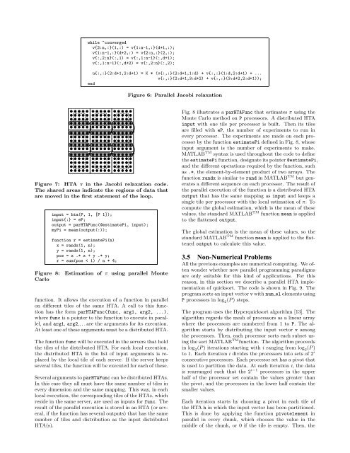
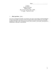
¡ ¡ ¡ ¡ ¡ ¡ ¡¡ ¡ ¡ ¡ ¡ ¡ ¡while ~convergedv{2:n,:}(1,:) = v{1:n-1,:}(d+1,:);v{1:n-1,:}(d+2,:) = v{2:n,:}(2,:);v{:,2:n}(:,1) = v{:,1:n-1}(:,d+1);v{:,1:n-1}(:,d+2) = v{:,2:n}(:,2);u{:,:}(2:d+1,2:d+1) = K * (v{:,:}(2:d+1,1:d) + v{:,:}(1:d,2:d+1) + ...v{:,:}(2:d+1,3:d+2) + v{:,:}(3:d+2,2:d+1));endFigure 6: Parallel Jacobi relaxation¨ ¨ ¨ ¨ ¨ ¨© © © © © © ©¨¨ ¨ ¨ ¨ ¨ ¨ ¨© © © © © ©©© © © © © ©© ¨ ¨ ¨ ¨ ¨ ¨ ¨¦ ¦ ¦ ¦ ¦ ¦§ § § § § § §¦¦ ¦ ¦ ¦ ¦ ¦ ¦§ § § § § §§§ § § § § §§ ¦ ¦ ¦ ¦ ¦ ¦ ¦¡ ¡ ¡ ¡ ¡ ¡ ¡¤ ¤ ¤ ¤ ¤ ¤¥ ¥ ¥ ¥ ¥ ¥ ¥¤¤ ¤ ¤ ¤ ¤ ¤ ¤¥ ¥ ¥ ¥ ¥ ¥¥¥ ¥ ¥ ¥ ¥ ¥¥ ¤ ¤ ¤ ¤ ¤ ¤ ¤ ¢ ¢ ¢ ¢ ¢ ¢£ £ £ £ £ £ £¢¢ ¢ ¢ ¢ ¢ ¢ ¢£ £ £ £ £ £££ £ £ £ £ ££ ¢ ¢ ¢ ¢ ¢ ¢ ¢Figure 7: HTA v in the Jacobi relaxation code.The shared areas indicate the regions of data thatare moved in the first statement of the loop.input = hta(P, 1, [P 1]);input{:} = eP;output = parHTAFunc(@estimatePi, input);myPi = mean(output(:));function r = estimatePi(n)x = randx(1, n);y = randx(1, n);pos = x .* x + y .* y;r = sum(pos < 1) / n * 4;Figure 8: Estimation of π using parallel MonteCarlofunction. It allows the execution of a function in parallelon different tiles of the same HTA. A call to this functionhas the form parHTAFunc(func, arg1, arg2, ...),where func is a pointer to the function to execute in parallel,and arg1, arg2,. . . are the arguments for its execution.At least one of these arguments must be a distributed HTA.The function func will be executed in the servers that holdthe tiles of the distributed HTA. For each local execution,the distributed HTA in the list of input arguments is replacedby the local tile of each server. If the server keepsseveral tiles, the function will be executed for each of these.Several arguments toparHTAFunc can be distributed HTAs.In this case they all must have the same number of tiles inevery dimension and the same mapping. This way, in eachlocal execution, the corresponding tiles of the HTAs, whichreside in the same server, are used as inputs for func. Theresult of the parallel execution is stored in an HTA (or several,if the function has several outputs) that has the samenumber of tiles and distribution as the input distributedHTA(s).Fig. 8 illustrates a parHTAFunc that estimates π using theMonte Carlo method on P processors. A distributed HTAinput with one tile per processor is built. Then its tilesare filled with eP, the number of experiments to run inevery processor. The experiments are made on each processorby the function estimatePi defined in Fig. 8, whoseinput argument is the number of experiments to make.MATLAB TM syntax is used throughout the code to definetheestimatePi function, designate its pointer@estimatePi,and the different operations required by the function, suchas .*, the element-by-element product of two arrays. Thefunction randx is similar to rand in MATLAB TM but generatesa different sequence on each processor. The result ofthe parallel execution of the function is a distributed HTAoutput that has the same mapping as input and keeps asingle tile per processor with the local estimation of π. Tocompute the global estimation, which is the mean of thesevalues, the standard MATLAB TM function mean is appliedto the flattened output.The global estimation is the mean of these values, so thestandard MATLAB TM function mean is applied to the flattenedoutput to calculate this value.3.5 Non-Numerical ProblemsAll the previous examples are numerical computing. We oftenwonder whether new parallel programming paradigmsare only suitable for this kind of applications. For thisreason, in this section we describe a parallel HTA implementationof quicksort. The code is shown in Fig. 9. Theprogram sorts an input vectorvwithnum el elements usingP processors in log 2 (P) steps.The program uses the Hyperquicksort algorithm [13]. Thealgorithm regards the mesh of processors as a linear arraywhere the processors are numbered from 1 to P. The algorithmstarts by distributing the input vector v amongthe processors. Then, each processor sorts each subset usingthe sort MATLAB TM function. The algorithm proceedsin log 2 (P) iterations starting with i ranging from log 2 (P)to 1. Each iteration i divides the processors into sets of 2 iconsecutive processors. Each processor set has a pivot thatis used to partition the data. At each iteration i, the datais rearranged such that the 2 i−1 processors in the upperhalf of the processor set contain the values greater thanthe pivot, and the processors in the lower half contain thesmaller values.Each iteration starts by choosing a pivot in each tile ofthe HTA h in which the input vector has been partitioned.This is done by applying the function pivotelement inparallel in every chunk, which chooses the value in themiddle of the chunk, or 0 if the tile is empty. Then, the
Page 1: The Hierarchically Tiled Arrays Pro
Page 6 and 7: num_el = length(v);h = hta(v, {1:ce
Page 8 and 9: Our toolbox has been implemented an
Page 10 and 11: Speedup9876543210HTAMPIep mg ft_1d
Page 12: [9] W. Gropp, E. Lusk, and A. Skjel

The Hierarchically Tiled Arrays Programming Approach

Create successful ePaper yourself

Delete template?

Save as template?