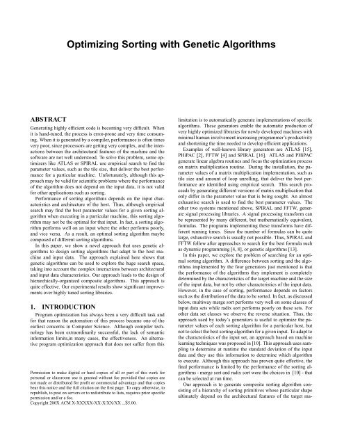
Optimizing Sorting with Genetic Algorithms - Polaris

Optimizing Sorting with Genetic Algorithms
ABSTRACT
Generating highly efficient code is becoming very difficult. When
it is hand-tuned, the process is error-prone and very time consuming.
When it is generated by a compiler, performance is often times
very poor, since processors are getting very complex, and the interactions
between the architectural features of the machine and the
software are not well understood. To solve this problem, some optimizers
like ATLAS or SPIRAL use empirical search to find the
parameter values, such as the tile size, that deliver the best performance
for a particular machine. Unfortunately, although this approach
may be valid for scientific problems where the performance
of the algorithm does not depend on the input data, it is not valid
for other applications such as sorting.
Performance of sorting algorithms depends on the input characteristics
and architecture of the host. Thus, although empirical
search may find the best parameter values for a given sorting algorithm
when executing in a particular machine, this sorting algorithm
may not be the optimal for that input. In fact, a sorting algorithm
performs well on an input where the other performs poorly,
and vice versa. As a result, an optimal sorting algorithm maybe
composed of different sorting algorithms.
In this paper, we show a novel approach that uses genetic algorithms
to design sorting algorithms that adapt to the host machine
and input data. The approach explained here shows that
genetic algorithms can be used to explore the huge search space,
taking into account the complex interactions between architectural
and input data characteristics. Our approach leads to the design of
hierarchically-organized composite algorithms. This approach is
quite effective. Our experimental results show significant improvements
over highly tuned sorting libraries.
1. INTRODUCTION
Program optimization has always been a very difficult task and
for that reason the automation of this process became one of the
earliest concerns in Computer Science. Although compiler technology
has been extraordinarily successful, the lack of semantic
information limits,in many cases, the effectiveness. An alternative
program optimization approach that does not suffer from this
Permission to make digital or hard copies of all or part of this work for
personal or classroom use is granted without fee provided that copies are
not made or distributed for profit or commercial advantage and that copies
bear this notice and the full citation on the first page. To copy otherwise, to
republish, to post on servers or to redistribute to lists, requires prior specific
permission and/or a fee.
Copyright 200X ACM X-XXXXX-XX-X/XX/XX ...$5.00.
limitation is to automatically generate implementations of specific
algorithms. These generators enable the automatic production of
very highly optimized libraries for newly developed machines with
minimal human involvement increasing programmer’s productivity
and shortening the time needed to develop efficient applications.
Examples of well-known library generators are ATLAS [15],
PHiPAC [2], FFTW [4] and SPIRAL [16]. ATLAS and PHiPAC
generate linear algebra routines and focus the optimization process
on matrix multiplication routine. During the installation, the parameter
values of a matrix multiplication implementation, such as
tile size and amount of loop unrolling, that deliver the best performance
are identified using empirical search. This search proceeds
by generating different versions of matrix multiplication that
only differ in the parameter value that is being sought. An almost
exhaustive search is used to find the best parameter values. The
other two systems mentioned above, SPIRAL and FFTW, generate
signal processing libraries. A signal processing transform can
be represented by many different, but mathematically equivalent,
formulas. The programs implementing these transforms have different
running times. Since the number of formulas can be quite
large, exhaustive search is usually not possible. Thus, SPIRAL and
FFTW follow after approaches to search for the best formula such
as dynamic programming [4, 8], or genetic algorithms [13].
In this paper, we explore the problem of searching for an optimal
sorting algorithm. A difference between sorting and the algorithms
implemented by the four generators just mentioned is that
the performance of the algorithms they implement is completely
determined by the characteristics of the target machine and the size
of the input data, but not by other characteristics of the input data.
However, in the case of sorting, performance depends on factors
such as the distribution of the data to be sorted. In fact, as discussed
below, multiway merge sort performs very well on some classes of
input data sets while radix sort performs poorly on these sets. For
other data set classes we observe the reverse situation. Thus, the
approach used by today’s generators is useful to optimize the parameter
values of each sorting algorithm for a particular host, but
not to select the best sorting algorithm for a given input. To adapt to
the characteristics of the input set, an approach based on machine
learning techniques was proposed in [10]. This approach uses sampling
to determine at runtime the standard deviation of the input
data and they use this information to determine which algorithm
to execute. Although this approach has proven quite effective, the
final performance is limited by the performance of the sorting algorithms
- merge sort and radix sort were the choices in [10] - that
can be selected at run time.
Our approach is to generate composite sorting algorithm consisting
of a hierarchy of sorting primitives whose particular shape
ultimately depend on the architectural features of the target ma-

chine and the characteristics of the input data. The intuition behind
this is that different partitions of the input data benefit more from
different sorting algorithms and, as a result, the optimal sorting algorithm
should be the composition of these different sorting algorithms.
Beside the sorting primitives, the generated code contains
selection primitives that adapt at runtime to the characteristics of
the input. The search for the optimal composite sorting algorithm
is done using genetic algorithms [5]. Genetic algorithms have also
been used to search for the appropriate formula in SPIRAL [13]
and to optimize compiler heuristics [14].
Our results show that this approach is very effective. The best
composite algorithm we have been able to generate are up to 42%
faster than the best “pure” sorting algorithms.
The rest of this paper is organized as follows. Section 2 discusses
the primitives that we use to build sorting algorithms. Section
3 explain why we chose genetic algorithms for the search and
explains some details of the algorithm that we implemented. Section
4 shows performance results, and finally Section 5 presents the
conclusion.
2. SORTING PRIMITIVES
In this section, we describe the building blocks of our composite
sorting algorithms. These primitives were selected based on experiments
with different sorting algorithms and the study of the factors
that affect their performance. A summary of the results of these experiments
is presented in Figure 1 which plots the execution time
of three sorting algorithms against the standard deviation of the
keys to be sorted. Results are shown for two platforms, Intel Pentium
III Xeon and Sun Ultra-Sparc III, and for two data sets sizes
2M (figures on the left) and 16M (figures on the right). The three
algorithms are: quicksort [6, 12], a cache-conscious radix sort (CCradix)
[7], and multiway merge sort [9]. Figure 1 shows that for
2M records, the best sorting algorithm is either quicksort or CCradix.
However, for 16M records, multiway merge or CC-radix
are the best algorithms. The input characteristics that determine
when CC-radix is the best algorithm is the standard deviation of
the records to be sorted. CC-radix is better when the standard deviation
of the records if high, because if the values of the elements in
the input data are concentrated around some values, it is more likely
that most of these elements end up in a small number of buckets.
Thus, more partitions will have to be applied before the buckets fit
into the cache and therefore more cache misses are incurred during
the partitioning. On the other hand, if we compare the performance
on the two platforms we can see that, although the general trend of
the algorithms is always the same, the performance crossover point
occurs at different points.
Other experiments, not described in detail here, have shown that
the performance of the pure quicksort algorithm can be improved
when combined with other algorithms. For example, experimental
results show that when the partition is smaller than a certain
threshold (whose value depends on the target platform), it is better
to use insertion sort or register sort [10], instead of continuing
to recursively apply quicksort. Register sort is a straight-line code
algorithm that performs compare-and-swap of values stored in processor
registers [9]. The idea of using insertion sort to sort the small
partitions that appear after the recursive calls of quicksort was also
used in [12] to improve the performance of quicksort.
In this paper, we search for an optimal algorithm by building
composite sorting algorithms. This approach was also followed in
[3] to classify several sorting algorithms. We use two types of primitives:
sorting and selection primitives. Sorting primitives represent
a pure sorting algorithm that involves partitioning the data, such as
radix sort, merge sort and quicksort. Selection primitives represent
a process to be executed at runtime that dynamically decide which
sorting algorithm to apply.
The composite sorting algorithm we used in this study assumes
that the data is stored in consecutive memory locations. The data
is then recursively partitioned using one of three partitioning methods.
The recursive partitioning ends when a leaf sorting algorithm
is applied to the partition. We now describe the three partitioning
primitives followed by a description of the two leaf sorting primitives.
1. Divide − by − Value(DV)
This primitive corresponds to the first phase of quicksort which,
in the case of a binary partition, selects a pivot and reorganizes
the data so that the first part of the vector contains the keys with
values smaller than the pivot, then comes the pivot, and the third
part contains the rest of the keys. In our work, the DV primitive
can partition the set of records into two or more parts using a
parameter np, that specifies the number of pivots. Thus, this
primitive divide the input set in np +1partitions, and rearranges
the data around the np pivots.
2. Divide − by − position (DP)
This primitive corresponds to multiway merge sort and the initial
step just breaks the input array of keys into two or more partitions
or subsets. It is implicit in the DP primitive that, after all the partitions
have been processed, the partitions are merged to obtain a
sorted array. The merging is accomplished using a heap or priority
queue [9]. The merge operation works as follows. At the
beginning the leaves in the heap are the first elements of all the
subsets. Then, pairs of leaves are compared, the larger/smaller is
promoted to the parent node, and a new element from the subset
of the promoted element becomes a leaf. This is done recursively
until the heap is full. After that, the element at the top of
the heap is extracted, placed in the destination vector, a new element
from the corresponding subset is promoted and the process
repeats again. Figure 2 shows a picture of the heap.
Heap
2*p−1 nodes
...
Sorted Sorted
Sorted Sorted
...
Subset Subset Subset Subset
p Subsets
Figure 2: Multiway Merge.
The heap is implemented as an array where siblings are located
in consecutive array elements. When merging using the heap,
The operation of finding the child with the largest/smallest key
is executed repetitively. If the number of children of each parent
is smaller than the number of nodes that fit in a cache line, the
cache line will be under-utilized. To solve this problem, if for
example the cache line is A bytes, and each node requires r bytes,
we use a heap with a fanout of A/r. That is, each parent of our

1.05e+09
Intel PIII Xeon (2M)
9.5e+09
Intel PIII Xeon (16M)
Execution Time (Cycles)
1e+09
9.5e+08
9e+08
8.5e+08
8e+08
7.5e+08
7e+08
6.5e+08
Execution Time (Cycles)
9e+09
8.5e+09
8e+09
7.5e+09
7e+09
6.5e+09
6e+09
5.5e+09
6e+08
100 1000 10000 100000 1e+06 1e+07 1e+08
Standard Deviation
Quicksort CC-radix Multiway merge
5e+09
100 1000 10000 100000 1e+06 1e+07 1e+08
Standard Deviation
Quicksort CC-radix Multiway merge
1.1e+09
Sun UltraSparc III (2M)
1.1e+10
Sun UltraSparc III (16M)
Execution Time (Cycles)
1e+09
9e+08
8e+08
7e+08
6e+08
Execution Time (Cycles)
1e+10
9e+09
8e+09
7e+09
6e+09
5e+08
100 1000 10000 100000 1e+06 1e+07 1e+08
Standard Deviation
Quicksort CC-radix Multiway merge
5e+09
100 1000 10000 100000 1e+06 1e+07 1e+08
Standard Deviation
Quicksort CC-radix Multiway merge
Figure 1: The effect of the standard deviation on the performance of the sorting algorithms. Plots on the left column correspond to
2M keys, while plots on the right column correspond to 16M keys.
heap has A/r children. Figure 3 shows a 4-way heap. This takes
maximum advantage of spatial locality when the cache line can
accommodate exactly four nodes. Of course, for this to be true,
the array structure implementing the heap needs to be properly
aligned.
Heap
00000 11111
00000 11111
00000 11111
00000
11111
00000
11111
00000
11111
Cache line
00000
11111
00000
11111
00000
11111
00000
11111
00000
11111
00000
11111
00000
11111
00000
11111
00000
11111
...
...
00000 11111
00000 11111
11111
00000
Cache line
000000
111111
000000
111111
000000
111111
Cache line
Figure 3: Fill as many as possible child nodes into a cache line.
The DP primitive has two parameters: size that specifies the size
of each partition or subset, and fanout, that specifies the number
of children of each node of the heap.
3. Divide − by − radix (DR)
The Divide-by-Radix primitive corresponds to a step of the radix
sort algorithm. The DR primitive distributes the records to be
sorted into buckets depending on the value of a digit in the record.
Thus, if we use a radix of r bits, the records will be distributed
into 2 r sub-buckets based on the value of a digit of r bits. Figure
4 presents an example where the DR primitive is applied to
the second most significant digit. The example assumes base 8
numbers, and the radix size is therefore 3 bits. An important
feature of this primitive is that it is a non-comparison based algorithm.
The DR primitive has a parameter radix that specifies the size of
the radix in number of bits. The position of the digit in the record
is not specified in the primitive, but is determined by the system.
Conceptually, the system keeps a counter for each partition
which identifies the position where the digit to be used for radix
sort starts. Every partition that is created inherit the counter of its
parents. The counter is initialized at zero and is incremented by
the size of the radix (in number of bits) each time a DR primitive
is applied.
113
142
127
145
170
142
177
171
115
117
137
Divide by Radix
applied to the second
most significant digit
113
115
117
127
137
142
145
142
170
177
171
Figure 4: Divide by radix primitive applied to the most significant
digit.
Apart from these primitives we also have recursive primitives that
will be applied until the partition is sorted. We call them leaf
primitives.

4. Leaf − Divide − by − Value(LDV)
This primitive specifies that the DV primitive must be applied
recursively to sort the partitions. However, when the size of the
partition is smaller than a certain threshold, this LDV primitive
uses the in-place register sorting algorithms to sort the records in
that partition. LDV has two parameters: np, which specifies the
number of pivots as in the DV primitive, and threshold, which
specifies the partition size below the one the sorting networks
algorithm is applied.
5. Leaf − Divide − By − Radix (LDR)
This primitive specifies that the DR primitive is used to sort the
remaining subsets. LDR has two parameters: radix and threshold.
As in LDV, the threshold is used to specify the size of the partition
to commute to register sorting.
Notice that although the number and type of sorting primitives
could be different, we have chosen to use these five because they
represent the pure algorithms that obtained better results in our experiments.
Other sorting algorithms such as heap sort and merge
sort, never obtained the performance of the sorting algorithms selected
here. Merge sort is not considered as an alternative to sort
leaves because we have found it to be slower than quicksort and
radix sort for small partitions.
All the sorting primitives have parameters whose most appropriate
value will depend on architectural features of the target machine.
Consider, for example, the DP primitive. The size parameter
is related to the size of the cache, while the fanout is related
to the number of elements that fit in a cache line. Similarly, the np
and radix of the DV and DR primitives are related to the cache
size. However, the precise value of these parameters cannot be easily
determined. For example, the relation between np and the cache
size is not straightforward, and the optimal value may also vary depending
on the number of keys to sort. The parameter threshold
is related to the number of registers.
In addition to the sorting primitives, we also use selection primitives.
The selection primitives can be used at runtime to determine,
based on the characteristics of the input, the sorting primitive to
apply to each sub-partition of a given partition. Based on the results
shown in Figure 1, these selection primitives were designed to
take into account the number of records in the partition and/or their
standard deviation. These selection primitives are:
1. Branch − by − Size (BS)
As shown in Figure 1, the number of records to sort is an input
characteristic that determines the relative performance of our
sorting primitives. This BS primitive, will be used to select different
paths based of the size of the partition. Thus, this BS primitive,
has one or more (size1, size2, ...) parameters to choose the
path to follow. The size values are sorted and used to select n+1
possibilities (less than size1, between size1 and size2, ..., larger
than sizen).
2. Branch − by − Entropy (BE)
Besides the size of the partition, the other input characteristic
that determines the performance of the above sorting primitives
is the standard deviation. However, instead of using the standard
deviation to select the different paths to follow we use, as was
done in [10], the notion of entropy from information theory.
There are several reasons to use entropy instead of standard deviation.
Standard deviation is expensive to compute since it requires
several floating point operations per record. Although, as
< S1
LDR r=5, t=0
(a) CC−radix with
radix 5 for all the digits
DR r=8
B Size
LDR r=4, t=16 LDR r=8, t=16
(b)CC− radix with
different radix sizes
< V1
DP s=32K, f=4
B Entropy
>=V1 && V2
LDV np=2, t=8 B Size LDR r=8, t=16
>= S1 < S1
>=S1
LDR r=8, t=16 LDV np=2, t=8
(c) Composite sorting algorithm
Figure 5: Tree based encoding of different sorting algorithms.
can be seen in Figure 1, the standard deviation is the factor that
determines when CC-radix is the best algorithm, in practice the
behavior of CC-radix depends, more than on the standard deviation
of the the records to sort, on how much the values of each
digit are spread out. The entropy of a digit position will give us
this information. CC-radix sort distributes the records according
to the value of one of the digits. If the values of this digit are
spread out, the entropy will be high and the resulting sub-buckets
will contain fewer elements, and, as a result, the sub-bucket will
be more likely to fit in the cache. When each of these sub-buckets
is partitioned again according to the next digit, the cache misses
will be low. If, however, the entropy is low, it will mean the opposite.
Most of the records will end up in the same sub-bucket,
which very likely will not fit in cache. When this sub-bucket is
sorted again, it will result in cache misses and, as a result, lower
performance.
To compute the entropy, at runtime we need to scan the input
set and compute the number of keys that have a particular value
for each digit position. For each digit, the entropy is computed
as ∑ i −P i ∗ log 2 P i , where P i = c i /N , c i is the number of
keys with value i in that digit, and N is the total number of keys.
The result is a vector of entropies, where each element of the
vector represents the entropy of a digit position in the key. We
then compute S, as the inner product of the computed entropy
∑
vector (E i ) and a weight vector (W i ), whose values we fix: S =
i E i ∗ W i . The resulting S value is used to select the path to
proceed with the sorting.
Primitive
DV
DP
DR
LDV
LDR
BN
BE
Parameters
np: number of pivots
t: threshold when to use in-place register sort
s: partition size
f: fanout of the heap
r: radix size is r bits
np: number of pivots
t: threshold when to use in-place register sort
r: radix size is r bits
n: there are n +1branches
size: n size thresholds for to n +1branches
n: there are n +1branches
ent: n entropy thresholds for to n +1branches
Table 1: Summary of primitives and their parameters.
A summary of the primitives and their parameters is listed in Table
1. We will use the seven primitives presented here (5 sorting
primitives and 2 selection primitives) to build sorting algorithms.

Figure 5 shows an example where different sorting algorithms are
encoded using a tree based schema using the different primitives.
Figure 5-(a) shows the encoding corresponding to a pure radix sort
algorithm, where all the partitions are sorted using the same radix
of 2 5 . Our DR primitive sorts the data according to the value of
the most left digit of a given radix that has not been processed yet.
Figure 5-(b) shows the encoding of an algorithm with radix size of
either 2 4 or 2 8 depending on the number of records of the partition.
Radix 2 4 is used when the number of records is V1) a radix sort using radix 2 8 is applied.
Otherwise, if the entropy is between V 1 and V 2, another selection
is made based on the size of the partition. If the size is less than S1,
a radix sort with radix 2 8 is applied. Otherwise a three-way quicksort
is applied. At the end, each subset is sorted, but they need to be
sorted among themselves. For that, the initial subsets are merged
using a heap like the one in Figure 2, with a fanout of 4, which is
the parameter value of the DP primitive.
The primitives we are using cannot generate all possible sorting
algorithm, but by combining them they can build a much larger
space of sorting algorithms than that containing only the traditional
pure sorting algorithms like quicksort or radix sort. Also, by changing
the parameters in the sorting and selection primitives, we can
adapt to the architecture of the target machine and to the characteristics
of the input data.
3. GENETIC SORTING
In this section we explain the use of genetic algorithms to optimize
sorting. We first explain why we believe that genetic algorithms
are a good search strategy and then explain how to use them.
3.1 Why Use Genetic Algorithms
Traditionally, the complexity of sorting algorithms has been studied
in terms of the number of comparisons or the number of iterations
executed [9]. These studies assume that the time to access
each element is the same. This assumption, however, is not true in
today’s processors because of their deep cache hierarchy. In fact,
the architectural features of new processors complicate the design
of sorting algorithms. For example, suppose that the optimal sorting
algorithm for a Itanium2 is quicksort. This comparison-based
algorithm could be slow on a Pentium4 that has a trace cache because
the trace cache can not make good predictions because of
the many branch instructions in a comparison-based sorting algorithm,
and therefore, a non-comparison based radix sort algorithm
could perform much better. Unfortunately, no analytical model has
been developed to predict the performance of sorting algorithms
based on the architectural features of the machine. Furthermore,
even if we were able to predict the best sorting algorithm for a particular
platform, we still would have to find the parameter values
that would deliver the best performance in that platform given its
cache size, cache line size, number of registers, and so on. Recent
experimental results with ATLAS have proven that doing an empirical
search of parameter values such as tile size and amount of
unroll can improve performance significantly relative to using the
values selected by compilers [17]. For applications such as sorting,
the difference should be even greater since current analysis techniques
are not powerful enough to support automatic restructuring
of sorting algorithms. For example, it is not generally feasible to
automatically determine that it is possible to change the partition
size for multiway merge sort.
The approach that we followed is to use genetic algorithms to
search for an optimal sorting algorithm by combining the sorting
and selection primitives designed in Section 2. During the process,
we also search for the parameter values of the primitives that better
suit to the architectural features of the machine and the characteristics
of the input set.
The reason to use the sorting and selection primitives to build
an effective sorting algorithm is that a pure algorithm is unlikely to
be optimal. An optimal sorting algorithm is more likely a composite
algorithm consisting of a hierarchy of sorting algorithms whose
particular shape depends on the characteristics of the input to sort
and the architecture of the target machine. The intuition behind this
is that different partitions will benefit more from different sorting
algorithms, and as a result the optimal sorting algorithm should be
the composition of these different sorting algorithms.
There are several reasons why we have chosen genetic algorithms
to perform the search. We discuss them next.
• Using the primitives in Section 2, the sorting algorithms can
be encoded using a tree based schema, as shown in Figure 5.
Genetic algorithms can be easily used to search in this space
for the most appropriate tree shape and parameter values. Other
loop-based search mechanisms, such as hill climbing, can search
for the appropriate parameter values, but they are not adequate
for searching the optimal tree.
• The search space of sorting algorithms that can be derived using
the seven primitives in Section 2 is too large for exhaustive
search. For example suppose that each primitive has only one
parameter, and each parameter can only take two different values.
Assuming a tree with 6 nodes, and ignoring the structural
differences, the number of possible trees is (7 ∗ 2) 6 = 7529536.
• Genetic algorithms preserves the best subtrees and give those
subtrees more chances to reproduce. Sorting algorithms can take
advantage of this since a sub-tree is also a sorting algorithm.
Suppose that a sub-tree is optimal when sorting small number
of records. It can then be used as a building block for a sorting
algorithm for larger number of records. This is the idea behind
dynamic programming, where the solution to a large problem
is composed of the best solutions found for smaller problems.
However, genetic algorithms are more flexible. Genetic algorithms
can, like dynamic programming, obtain an optimal sorting
algorithm for 16M records which uses the best sorting algorithm
for 4M records. However, genetic algorithms are not
restricted to using the solution found for a smaller problem as
the building blocks to solve a larger problem. They may also
find that the best solution for sorting 16M records has nothing to
do with the one found for 4M records.
In our case, genetic programming maintains a population of tree
genomes. Each tree genome is an expression that represents a sorting
algorithm. The tree genomes are selected for reproduction
(called crossover) proportional to their level of fitness. The expressions
better solving the problem are given more opportunities
to produce offsprings. Genetic programming also randomly mutate
some expressions to create a possibly better genome.

3.2 Optimization of Sorting with Genetic Algorithms
3.2.1 Encoding
As discussed above we use a tree based schema where the nodes
of the tree are sorting and selection primitives.
3.2.2 Operators
Genetic operators are used to derive new offsprings and introduce
changes in the population. Crossover and mutation are the two
operators that most genetic algorithms use. Crossover exchanges
subtrees from different trees. Mutation operator applies changes to
a single tree. Next, we explain how we apply these two operators.
Crossover
The purpose of crossover is to generate new offsprings that have
better performance than their parents. This is likely to happen when
the new offsprings inherit the best subtrees of the parents.
In this paper we use single-point cross-over, since it can preserve
the whole subtree without changing its structure. Figure 6 shows
an example of single-point crossover.
DV
LDV
Parent trees
DP
DR
DR
BE
LDV
LDR
DR
Offsprings
Figure 6: Crossover of sorting trees.
Mutation
Mutation works on a single tree, where it produces some changes,
introducing some diversity in the population. This operator, however,
does not produce new offsprings. Mutation prevents the population
from permanent fixation at any particular generation [1].
This, to some extent, avoids the local optimal problem. Mutation
changes the parameter values hoping to find better ones. Our mutation
operator can perform the following changes:
1. Change the values of the parameters in the sorting and selection
primitive nodes. The parameters are changed randomly but the
new value is close to the old one, with the hope that the parameter
will converge to the best values.
2. Flip: Exchange two subtrees. This type of mutation can help
in cases like the one shown in Figure 7-(a) where a subtree that
is good to sort sets of less than 4M records is being applied to
larger sets. By exchanging the subtrees we can correct this type
of misplacement.
3. Grow: Add a new subtree. This type of mutation is helpful
when more partitioning is required along one path in the tree.
Figure 7-(b) shows an example of this mutation.
4. Truncate: Remove a subtree. Unnecessary subtrees can be deleted
with this operation.
LDV
DP
DR
BE
DV
LDV
LDR
Optimal subtee
for 4 M records
4M
Subtree A
BS
BS
Optimal subtee
for 4 M records
Exchange subtrees
4M
(a)
Subtree A
Optimal subtee
for 4 M records
Add a new
subtree
DP s=4M records
Optimal subtee
for 4 M records
Figure 7: Mutation operator. (a)-Exchange subtrees. (b)-Add
a new subtree.
3.2.3 Fitness Function
The fitness function determines the probability for an individual
to reproduce in the population. The higher the fitness of an individual,
the higher the chances it will reproduce and mutate.
In our case, performance will be used as the fitness function.
However, the following two considerations have been taken into
account in the design of our fitness function:
1. We are searching for a sorting algorithm that performs well
across all possible inputs. Thus, the average performance of
a tree can be used as its base fitness. However, we also want
the sorting algorithm to consistently perform well across inputs.
Thus, the tree with a variable performance is penalized with a
factor that depends on the standard deviation of its performance
when sorting the test inputs.
2. In the first generations, the fitness variance of the population
is high, that is, a small number of sorting trees have a much
better performance than the other ones. If our fitness function
was directly proportional to the performance of the tree, most of
the offsprings would be the descendants of these few trees, since
they would have a much higher probability to reproduce. As a result,
these offsprings would soon occupy most of the population.
This could result in premature convergence, which would prevent
the system from exploring areas of the search space outside the
neighborhood of the highly fit trees. To address this problem, our
fitness function uses the performance order or rank of the sorting
trees in the population. By using the performance ranking, the
absolute performance difference between trees is not considered
and the trees with lower performance have more probability to
reproduce than if the absolute performance value had been used.
This avoids the problem of early convergence and of convergence
to a local optimum.
3.2.4 Evolution Algorithm
An important decision is to choose the appropriate evolution algorithm.
The evolution algorithm determines how many offsprings
will be generated, how many individuals of the current generation
will be replaced and so on. The search for the optimal sorting algorithm
is an incremental learning problem and, as such, what has
already been learned should be remembered and used later.
In this work we use a steady-state evolution algorithm. For each
generation, only a small number of the least fit individuals in the
current generation are replaced by the new generated offsprings.
(b)

Genetic Algorithm {
P = Initial Population
While (stopping criteria is false) do {
• Apply mutation and cross-over and generate set
M of B individuals
• P=P∪ M
• S = Input set with different sizes and different
standard deviations
• Use each genome of P to sort each element S
• Apply fitness function to remove the B least fit
individuals
}
}
of generations. 1 However, despite the limited scope of the search,
significant improvements have been obtained as we will show below.
The performance convergence curve presented in Section 4.3
indicates that further improvements are likely if more generations
or larger populations was used.
Parameters for Genetic algorithm
Population Size 20
#Generations 16
#Generated offsprings 12
Mutation Rate Probability 30%
#Training input sets 12
Figure 8: Genetic Algorithm used to find a sorting algorithm
that adapts to the host machine and input characteristics
Table 3: Parameters for the Evolving Genetic Algorithm. The
parameters correspond to one generation.
As a result, many of the individuals from the previous population
are likely to survive.
Figure 8 shows the code for the steady-state evolving algorithm
that we use to generate a sorting algorithm. Each generation, a fixed
number of new offsprings will be generated through cross-over and
some individuals will mutate as explained above. The fitness function
will be used to select the individuals to which the mutation and
cross-over operators are applied. Then, several input sets with different
characteristics (standard deviation and number of records)
will be generated and used to train the sorting trees (parents and
new offsprings) of each generation. The performance obtained by
each sorting algorithm will be used by the fitness function to decide
which are the least fit individuals and remove them from the
population. The number of individuals removed is the same as the
number generated. That way, the number of individuals remains
constant across generations.
Several criteria can be chosen as stopping criteria such as stop
after a number of generations, or stop when the performance has
not improved more than a certain percentage in the last number of
generations. The stopping criteria and initial population that we use
will be discussed in the next section.
4. EVALUATION
In this section we evaluate our approach of using genetic algorithms
to optimize sorting algorithm. In Section 4.1 we discuss
the environmental setup that we use for the evaluation. Section 4.2
presents performance results. Section 4.3 studies the convergence
of the performance results and, finally, Section 4.4 describes each
the the best sorting tree obtained for target platforms.
4.1 Environmental Setup
We evaluated our approach at five different platforms: AMD
Athlon MP, Sun UltraSparc III, Intel Itanium 2, Intel Pentium 4 and
SGI R12000. Table 2 lists for each platform the main architectural
parameters, the operating system, the compiler and the compiler
options used for the experiments.
For the evaluation we follow the evolution genetic algorithm in
Figure 8. Table 3 summarizes the parameter values that we have
used for the experiments. We use a population of 20 sorting trees,
and we let them evolve using the steady-state algorithm for 16 generations.
Due to the long running times that our experiments require,
we only present results for this small population and number
Our genetic algorithm searches for both the structure of the tree
and the parameter values. Thus, a high replacement rate is necessary
to guarantee that an appropriate parameter value can be reached
through random evolution. After a moderate number of preliminary
experiments, we have chosen a replacement rate of 60% which,
given a population size of 20 individuals, means that 12 new individuals
are generated through cross-over in each generation. The
mutation operator will mutate the new offsprings with a probability
of 30%. Also, 12 different input sets are generated in each
generation and used to test the 32 sorting trees (20 parents + 12
offsprings).
For the initial population we have chosen trees representing the
pure sorting algorithms of CC-radix [7], quicksort [12], multiway
merge [9], the adaptive algorithm in [10], and variations of these.
In all the platforms that we tried the initial individuals were quickly
replaced by better offsprings, although many subtrees of the initial
population were still present in the last generations.
4.2 Performance Results
We use genetic algorithms to search for either a specialized or
a general sorting algorithm. A specialized sorting algorithm is an
algorithm that has been optimized to sort data with some fixed characteristics
like number of records and/or standard deviation. A general
sorting algorithm is one that has been optimized for sorting
data regardless of their characteristics.
We start by comparing the performance of our genetic sorting
routine, our optimized quicksort, multi-way merge and the CCradix
with sorting routines from the Intel Math Kernel Library 6.1(MKL)
and the C++ STL. We tune our genetic sorting, quicksort, multiway
merge and CC-radix on Intel Itanium 2 and Intel Pentium 4.
The genetic sorting algorithm is tuned using the strategy presented
in this paper. The other algorithms are tuned using an empirical
search as discussed in [10]. Execution times were measured by
sorting several randomly-generated arrays containing 14M single
precision floating point values.
Figure 9 shows the performance of the six sorting routines. Our
optimized quicksort is faster than Intel MKL on the two platforms.
C++ STL is marginally slower than our quicksort at most points
on Intel Pentium 4 but faster than our quicksort on Intel Itanium 2.
However, C++ STL is much slower than the genetic sorting. The results
prove that the performance of our baseline algorithms, Quick
Sort, Multi-way Merge and CC-radix, are competitive with widely
1 For the final version of the paper we plan to present results for
larger populations and number of generations.

AMD Sun SGI Intel Intel
CPU Athlon MP UltraSparcIIIi R12000 Itanium 2 Pentium 4
Frequency 1.2GHz 1GHz 300MHz 1.5GHz 2GHz
L1d/L1i Cache 128KB 64KB/32KB 32KB/32KB 16KB/16KB 8KB/12KB
L2 Cache 256KB 1MB 4MB 256KB 512KB
Memory 1GB 4GB 1GB 8GB 512KB
OS RedHat9 SunOS5.8 IRIX64 v6.5 RedHat7.2 RedHat7.2
Compiler gcc3.2.2 Workshop cc 5.0 MIPSPro cc 7.3.0 gcc3.3.2 gcc3.3.1
Options -O3 -native -xO5 -O3 -TARG: -O3 -O3
platform=IP30
Table 2: Test Platforms. Intel Pentium 4 has a 8KB trace cache instead of a L1 instruction cache. Intel Itanium2 has a L3 cache of
6MB.
Execution Time (Cycles per key)
Execution Time (Cycles per key)
800
700
600
500
400
300
200
Intel Pentium 4
100
100 1000 10000 100000 1e+06 1e+07
1000
900
800
700
600
500
400
300
200
Quicksort
CC-radix
Standard Deviation
Multi-way Merge
Gene Sort
Intel MKL
C++ STL
100
100 1000 10000 100000 1e+06 1e+07
Quicksort
CC-radix
Intel Itanium 2
Standard Deviation
Multi-way Merge
Gene Sort
Intel MKL
C++ STL
Figure 9: Performance comparison with Intel Math Kernel Library
and C++ STL
used routines and and that the improvement on their performance
obtained by our genetic algorithm search is meaningful.
We now proceed to compare the sort algorithm generated by our
strategy with the three baseline algorithms. All the experiments
presented below sort records with two fields, a 32 bit integer key
and a 32 bit pointer. The reason for this structure is that, for the
long records typical of database, sorting is usually performed on an
array of tuples each containing a key and a pointer to the original
record [11]. We assume that this array has been created before our
library routines are called.
Next we show the performance of sorting algorithms that have
been using exclusively inputs of 14M records and the performance
of a second set of sorting algorithms that were tuned using input
data set sized ranging from 8M all the way to 16M records.
Figure 10 shows the performance of four different sorting algorithms:
Quicksort, CC-radix, Multiway Merge, and the sorting
algorithms generated using the genetic algorithm, Gene Sort, when
sorting input sets sized 14M. The Figure plots the execution time in
Cycles per key as the standard deviation changes from 512 to 8M.
The test inputs used to collect the data in Figure 10 were different
from the ones we used during the generation of the algorithm.
The use of genetic algorithms to optimize sorting results in a
significant improvement in performance. Our Gene sort (either the
specialized or the general form) usually performs better than the
best of the other three sorting algorithms. On Itanium2, which is the
platform with the minimum improvement, we obtain a 12% average
improvement. On the other platforms, the average improvement
over the best of the three algorithms is up to 42%.
There is not much difference between the performance of the
specialized and the general gene sort. The reason is that a sorting
algorithm can be good for a wide range of inputs. The specialized
genome intends to over-fit for the training data. It doesn’t necessarily
perform better than the general genome on the independent test
inputs.
4.3 Convergence Experiments
Figure 11 shows the speedup improvement for each generation.
The results are normalized with respect to the best sorting algorithm
in the initial population.
There are small up-and-downs in the speedup curves. That’s because
the test input data is different from the input data used for
training. The genetic algorithm always tunes for the data used during
training. Therefore, the best genome for generation n is not
necessarily better than the genome of generation n − 1 when sorting
the test data. It takes several generations and needs more random
trains to penalize the genomes selected because of the specific
sequence of values in the training set.
As the plot shows, for most platforms speedup remains relatively
stable for several generations and then it improves. The reason is
that it takes a while to “discover” a good genome. In that case,
the performance remains constant. Once, a new good individual
appears, it will reproduce fast, and, as a result, the performance of
the following generations will improve.
The Figure also shows that the speedup of Sun UltraSparcIIIi,
Athlon MP , Pentium 4 and SGI R12000 show no sign of convergence
after 16 generations. This leads us to believe that a higher
performance could be achieved by running the experiment for more
generations or with a larger population.

Execution Time (Cycles per key)
Execution Time (Cycles per key)
Execution Time (Cycles per key)
Execution Time (Cycles per key)
Execution Time (Cycles per key)
650
600
550
500
450
400
350
300
250
200
Sun UltraSparcIII
150
100 1000 10000 100000 1e+06 1e+07
600
550
500
450
400
350
300
250
Quicksort
CC-radix
Standard Deviation
Multi-way Merge
General Gene Sort
AMD Athlon MP
Special Gene Sort
200
100 1000 10000 100000 1e+06 1e+07
650
600
550
500
450
400
350
300
250
Quicksort
CC-radix
Standard Deviation
Multi-way Merge
General Gene Sort
Intel Itanium 2
Special Gene Sort
200
100 1000 10000 100000 1e+06 1e+07
600
550
500
450
400
350
300
Quicksort
CC-radix
Standard Deviation
Multi-way Merge
General Gene Sort
Intel Pentium 4
Special Gene Sort
250
100 1000 10000 100000 1e+06 1e+07
350
300
250
200
150
100
Quicksort
CC-radix
Standard Deviation
Multi-way Merge
General Gene Sort
SGI R12000
Special Gene Sort
50
100 1000 10000 100000 1e+06 1e+07
Quicksort
CC-radix
Standard Deviation
Multi-way Merge
General Gene Sort
Special Gene Sort
Speedup
1.5
1.45
1.4
1.35
1.3
1.25
1.2
1.15
1.1
1.05
1
0 2 4 6 8 10 12 14 16 18
Intel Itanium 2
Sun UltraSparcIIIi
Generation
SGI R12000
AMD Athlon MP
Intel Pentium 4
Figure 11: Performance of and the different sorting algorithms
as the standard deviation changes
4.4 Analyzing The Best Genome
Table 4 presents the shape of the best specialized genome and
the best general genome found in the experiments referred in Section
4.2. The string representation of the genome is of the form
(parent parameters (child 1) (child 2)...), where parameters are those
shown in Table 1. For example, ”(dr 17(be 2 300 600 (ldr 5)(dr 9(ldr
5))(lq 29))” means first partition the input array using the most significant
17-bits digit. Then, based on the entropy, we choose ”(ldr
5 20)” when the entropy is < 300, ”(dr 9(ldr 5 20))” when the entropy
is between 300 and 600, or ”(ldv 2 29))” when the entropy is
> 600. The triplet of ”(ldr 5 20)” means radix sort with radix 2 5
and threshold is 20. ”(ldv 1 29))” means using 1 pivot to divide
the partition and the threshold to use straight-line register sorting
is 29.
The best genomes seem puzzling at first. Only one best genome
uses branching primitive and divide − by − radix with a large
radix (> 2 10 ) is used as the first step on four platforms except on
Intel Itanium 2, where a divide − by − position (multiway merge)
is always favored. This is probably due to the size of the key to
be sorted. Since the key is only 32 bits long, divide − by − radix
with a large radix reduces the number of passes over the input array.
Though the first pass is expensive, the total number of instructions
executed decreases. However, we can expect different genome pattern
for 64-bit integer. If the values are not large enough to use
the most significant bits of 64-bit integer, that is, if the highest bits
of 64-bit integer are always 0, divide − by − radix with 18 bits
would place all input elements into the same bucket. However, using
a bigger digit is infeasible since divide − by − radix with a
bigger digit will increase the pressure on the memory requirement
for the auxiliary data structures. Assume the digit is n bits, the
size of the auxiliary counting array used in divide − by − radix
is O(2 n ). So the best genome for 64-bit keys is unlikely to evolve
into this pattern.
Our training sets for the genome are sized from 8M to 16M. After
divide − by − radix with a large radix, the number of elements in
each sub-bucket is expected to be small no matter the input set is
8M or 16M. Simpler algorithms are faster for small partitions. So,
practically no branching primitives are needed for sorting 32-bit
integer.
The presented diversity of the genomes highlights the importance
of building composite sorting algorithms using an automatic
search strategy. A manual tuning process can hardly lead to the best
genomes found in this study. The problem of manual tuning often
Figure 10: Performance of sorting algorithms as the standard
deviation changes

AMD Athlon MP Sun UltraSparcIIIi SGI R12000 Intel Itanium 2 Intel Pentium 4
Specialized (dr 18 (dr 6 (dr 15 (dr 10 (dr 17(be 2 300 600 (dp 169362 8 (dr 18 (ldr 5 20))
(ldr 5 20))) (dr 7 ))) (ldr 5 20)(dr 9(ldr 5 20))(ldv 1 29)) (ldr 5 20))
General (dr 17 (dr 10 (dv 2(dr 17 (dr 18 (dr 14)) (dp 246411 4 (dr 16 (dr 10
(ldr 5 20))) (dv 2(dr 15)))) (ldr 5 20)) (dr 6)))
Table 4: Best specialized genomes and best general genomes.
lies in the partial emphasis on some factors and ignorance of the
interaction between the algorithm and other factors. For example,
the design of CC-radix [7] focuses on reducing cache misses and
TLB misses. Therefore, only a moderate radix size is chosen. By
analyzing the automatically built sorting genomes, we can also get
better understanding of the interaction between the architecture and
the algorithms.
5. CONCLUSION
In this paper, we propose building composite sorting algorithms
from primitives to adapt to the target platform and the input data.
When combined, the primitives seam a huge space containing not
only the tradition sorting algorithms but many new sorting algorithms.
A genetic algorithm is applied to search for the best genome
in this space. The composite algorithm can be different from any
traditional sorting algorithm and automatically takes into account
the complex interactions between architecture and input data. Our
approach is quite successful. The generated sorting algorithm is
up to 42% faster than the highly tuned sorting libraries on the five
platforms on which we experimented.
6. REFERENCES
[1] T. Back, D. B. Fogel, and Z. Michalewicz. Evolutionary
Computation Vol. I & II. Institute of Physics Publishing,
2000.
[2] J. Bilmes, K. Asanovic, C. Chin, and J. Demmel. Optimizing
Matrix Multiply using PHiPAC: A Portable,
High-Performance, ANSI C Coding Methodology. In Proc.of
the 11th ACM International Conference on Supercomputing
(ICS), July 1997.
[3] J. Darlington. A Synthesis of Several Sorting Algorithms.
Acta Informatica, 11:1–30, 1978.
[4] M. Frigo. A Fast Fourier Transform Compiler. In Proc. of
Programing Language Design and Implementation, 1999.
[5] D. Goldberg. Genetic Algorithms in Search, Optimization,
and Machine Learning. Addison-Wesley, Reading, MA,
1989.
[6] C. Hoare. Quicksort. Computer, 5(4):10–15, April 1962.
[7] D. Jiménez-González, J. Navarro, and J. Larriba-Pey.
CC-Radix: A Cache Conscious Sorting Based on Radix Sort.
In Euromicro Conference on Parallel Distributed and
Network based Processing, pages 101–108, February 2003.
[8] H. Johnson and C. Burrus. The Design of Optimal DFT
Algorithms Using Dynamic Programming. IEEE
Transactions on Acoustics, Speech, and Signal Processing,
31:378–387, April 1983.
[9] D. Knuth. The Art of Computer Programming;
Volume3/Sorting and Searching. Addison-Wesley, 1973.
[10] X. Li, M. J. Garzarán, and D. Padua. A Dynamically Tuned
Sorting Library. In To appear in Proc. of the Int. Symp. on
Code Generation and Optimization, 2004.
[11] C. Nyberg, T. Barclay, Z. Cvetanovic, J. Gray, and D. Lomet.
AlphaSort: A RISC Machine Sort. In Proc. of the Sigmod
Conference, pages 233–242, 1994.
[12] R. Sedgewick. Implementing Quicksort Programs.
Communications of the ACM, 21(10):847–857, October
1978.
[13] B. Singer and M. Veloso. Stochastic Search for Signal
Processing Algorithm Optimization. In Proc. of
Supercomputig, 2001.
[14] M. Stepehnson, S. Amarasinghe, M.Martin, and U. O’Reilly.
Meta Optimiization: Improving Compiler Heuristics with
Machine Learning. In Proc. of Programing Language Design
and Implementation, June 2003.
[15] R. Whaley, A. Petitet, and J. Dongarra. Automated Empirical
Optimizations of Sofware and the ATLAS Project. Parallel
Computing, 27(1-2):3–35, 2001.
[16] J. Xiong, J. Johnson, R. Johnson, and D. Padua. SPL: A
Language and a Compiler for DSP Algorithms. In Proc. of
the International Conference on Programming Language
Design and Implementation, pages 298–308, 2001.
[17] K. Yotov, X. Li, G. Ren, M. Cibulskis, G. DeJong,
M. Garzaran, D. Padua, K. Pingali, P. Stodghill, and P. Wu.
A Comparison of Empirical and Model-driven Optimization.
In Proc. of Programing Language Design and
Implementation, pages 63–76, June 2003.