Optimizing Sorting with Genetic Algorithms - Polaris

More documents

Recommendations

Info

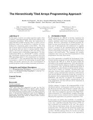
AMD Sun SGI Intel Intel CPU Athlon MP UltraSparcIIIi R12000 Itanium 2 Pentium 4 Frequency 1.2GHz 1GHz 300MHz 1.5GHz 2GHz L1d/L1i Cache 128KB 64KB/32KB 32KB/32KB 16KB/16KB 8KB/12KB L2 Cache 256KB 1MB 4MB 256KB 512KB Memory 1GB 4GB 1GB 8GB 512KB OS RedHat9 SunOS5.8 IRIX64 v6.5 RedHat7.2 RedHat7.2 Compiler gcc3.2.2 Workshop cc 5.0 MIPSPro cc 7.3.0 gcc3.3.2 gcc3.3.1 Options -O3 -native -xO5 -O3 -TARG: -O3 -O3 platform=IP30 Table 2: Test Platforms. Intel Pentium 4 has a 8KB trace cache instead of a L1 instruction cache. Intel Itanium2 has a L3 cache of 6MB. Execution Time (Cycles per key) Execution Time (Cycles per key) 800 700 600 500 400 300 200 Intel Pentium 4 100 100 1000 10000 100000 1e+06 1e+07 1000 900 800 700 600 500 400 300 200 Quicksort CC-radix Standard Deviation Multi-way Merge Gene Sort Intel MKL C++ STL 100 100 1000 10000 100000 1e+06 1e+07 Quicksort CC-radix Intel Itanium 2 Standard Deviation Multi-way Merge Gene Sort Intel MKL C++ STL 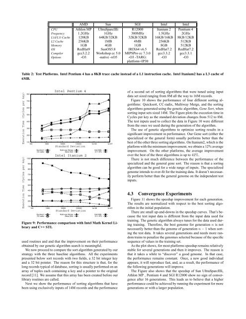Figure 9: Performance comparison with Intel Math Kernel Library and C++ STL used routines and and that the improvement on their performance obtained by our genetic algorithm search is meaningful. We now proceed to compare the sort algorithm generated by our strategy with the three baseline algorithms. All the experiments presented below sort records with two fields, a 32 bit integer key and a 32 bit pointer. The reason for this structure is that, for the long records typical of database, sorting is usually performed on an array of tuples each containing a key and a pointer to the original record [11]. We assume that this array has been created before our library routines are called. Next we show the performance of sorting algorithms that have been using exclusively inputs of 14M records and the performance of a second set of sorting algorithms that were tuned using input data set sized ranging from 8M all the way to 16M records. Figure 10 shows the performance of four different sorting algorithms: Quicksort, CC-radix, Multiway Merge, and the sorting algorithms generated using the genetic algorithm, Gene Sort, when sorting input sets sized 14M. The Figure plots the execution time in Cycles per key as the standard deviation changes from 512 to 8M. The test inputs used to collect the data in Figure 10 were different from the ones we used during the generation of the algorithm. The use of genetic algorithms to optimize sorting results in a significant improvement in performance. Our Gene sort (either the specialized or the general form) usually performs better than the best of the other three sorting algorithms. On Itanium2, which is the platform with the minimum improvement, we obtain a 12% average improvement. On the other platforms, the average improvement over the best of the three algorithms is up to 42%. There is not much difference between the performance of the specialized and the general gene sort. The reason is that a sorting algorithm can be good for a wide range of inputs. The specialized genome intends to over-fit for the training data. It doesn’t necessarily perform better than the general genome on the independent test inputs. 4.3 Convergence Experiments Figure 11 shows the speedup improvement for each generation. The results are normalized with respect to the best sorting algorithm in the initial population. There are small up-and-downs in the speedup curves. That’s because the test input data is different from the input data used for training. The genetic algorithm always tunes for the data used during training. Therefore, the best genome for generation n is not necessarily better than the genome of generation n − 1 when sorting the test data. It takes several generations and needs more random trains to penalize the genomes selected because of the specific sequence of values in the training set. As the plot shows, for most platforms speedup remains relatively stable for several generations and then it improves. The reason is that it takes a while to “discover” a good genome. In that case, the performance remains constant. Once, a new good individual appears, it will reproduce fast, and, as a result, the performance of the following generations will improve. The Figure also shows that the speedup of Sun UltraSparcIIIi, Athlon MP , Pentium 4 and SGI R12000 show no sign of convergence after 16 generations. This leads us to believe that a higher performance could be achieved by running the experiment for more generations or with a larger population.
Execution Time (Cycles per key) Execution Time (Cycles per key) Execution Time (Cycles per key) Execution Time (Cycles per key) Execution Time (Cycles per key) 650 600 550 500 450 400 350 300 250 200 Sun UltraSparcIII 150 100 1000 10000 100000 1e+06 1e+07 600 550 500 450 400 350 300 250 Quicksort CC-radix Standard Deviation Multi-way Merge General Gene Sort AMD Athlon MP Special Gene Sort 200 100 1000 10000 100000 1e+06 1e+07 650 600 550 500 450 400 350 300 250 Quicksort CC-radix Standard Deviation Multi-way Merge General Gene Sort Intel Itanium 2 Special Gene Sort 200 100 1000 10000 100000 1e+06 1e+07 600 550 500 450 400 350 300 Quicksort CC-radix Standard Deviation Multi-way Merge General Gene Sort Intel Pentium 4 Special Gene Sort 250 100 1000 10000 100000 1e+06 1e+07 350 300 250 200 150 100 Quicksort CC-radix Standard Deviation Multi-way Merge General Gene Sort SGI R12000 Special Gene Sort 50 100 1000 10000 100000 1e+06 1e+07 Quicksort CC-radix Standard Deviation Multi-way Merge General Gene Sort Special Gene Sort Speedup 1.5 1.45 1.4 1.35 1.3 1.25 1.2 1.15 1.1 1.05 1 0 2 4 6 8 10 12 14 16 18 Intel Itanium 2 Sun UltraSparcIIIi Generation SGI R12000 AMD Athlon MP Intel Pentium 4 Figure 11: Performance of and the different sorting algorithms as the standard deviation changes 4.4 Analyzing The Best Genome Table 4 presents the shape of the best specialized genome and the best general genome found in the experiments referred in Section 4.2. The string representation of the genome is of the form (parent parameters (child 1) (child 2)...), where parameters are those shown in Table 1. For example, ”(dr 17(be 2 300 600 (ldr 5)(dr 9(ldr 5))(lq 29))” means first partition the input array using the most significant 17-bits digit. Then, based on the entropy, we choose ”(ldr 5 20)” when the entropy is < 300, ”(dr 9(ldr 5 20))” when the entropy is between 300 and 600, or ”(ldv 2 29))” when the entropy is > 600. The triplet of ”(ldr 5 20)” means radix sort with radix 2 5 and threshold is 20. ”(ldv 1 29))” means using 1 pivot to divide the partition and the threshold to use straight-line register sorting is 29. The best genomes seem puzzling at first. Only one best genome uses branching primitive and divide − by − radix with a large radix (> 2 10 ) is used as the first step on four platforms except on Intel Itanium 2, where a divide − by − position (multiway merge) is always favored. This is probably due to the size of the key to be sorted. Since the key is only 32 bits long, divide − by − radix with a large radix reduces the number of passes over the input array. Though the first pass is expensive, the total number of instructions executed decreases. However, we can expect different genome pattern for 64-bit integer. If the values are not large enough to use the most significant bits of 64-bit integer, that is, if the highest bits of 64-bit integer are always 0, divide − by − radix with 18 bits would place all input elements into the same bucket. However, using a bigger digit is infeasible since divide − by − radix with a bigger digit will increase the pressure on the memory requirement for the auxiliary data structures. Assume the digit is n bits, the size of the auxiliary counting array used in divide − by − radix is O(2 n ). So the best genome for 64-bit keys is unlikely to evolve into this pattern. Our training sets for the genome are sized from 8M to 16M. After divide − by − radix with a large radix, the number of elements in each sub-bucket is expected to be small no matter the input set is 8M or 16M. Simpler algorithms are faster for small partitions. So, practically no branching primitives are needed for sorting 32-bit integer. The presented diversity of the genomes highlights the importance of building composite sorting algorithms using an automatic search strategy. A manual tuning process can hardly lead to the best genomes found in this study. The problem of manual tuning often Figure 10: Performance of sorting algorithms as the standard deviation changes
Page 1 and 2: Optimizing Sorting with Genetic Alg
Page 3 and 4: 1.05e+09 Intel PIII Xeon (2M) 9.5e+
Page 5 and 6: Figure 5 shows an example where dif
Page 7: Genetic Algorithm { P = Initial Pop

Optimizing Sorting with Genetic Algorithms - Polaris

Create successful ePaper yourself

Delete template?

Save as template?