Optimizing Sorting with Genetic Algorithms - Polaris
Optimizing Sorting with Genetic Algorithms - Polaris
Optimizing Sorting with Genetic Algorithms - Polaris

You also want an ePaper? Increase the reach of your titles
YUMPU automatically turns print PDFs into web optimized ePapers that Google loves.
4. Leaf − Divide − by − Value(LDV)<br />
This primitive specifies that the DV primitive must be applied<br />
recursively to sort the partitions. However, when the size of the<br />
partition is smaller than a certain threshold, this LDV primitive<br />
uses the in-place register sorting algorithms to sort the records in<br />
that partition. LDV has two parameters: np, which specifies the<br />
number of pivots as in the DV primitive, and threshold, which<br />
specifies the partition size below the one the sorting networks<br />
algorithm is applied.<br />
5. Leaf − Divide − By − Radix (LDR)<br />
This primitive specifies that the DR primitive is used to sort the<br />
remaining subsets. LDR has two parameters: radix and threshold.<br />
As in LDV, the threshold is used to specify the size of the partition<br />
to commute to register sorting.<br />
Notice that although the number and type of sorting primitives<br />
could be different, we have chosen to use these five because they<br />
represent the pure algorithms that obtained better results in our experiments.<br />
Other sorting algorithms such as heap sort and merge<br />
sort, never obtained the performance of the sorting algorithms selected<br />
here. Merge sort is not considered as an alternative to sort<br />
leaves because we have found it to be slower than quicksort and<br />
radix sort for small partitions.<br />
All the sorting primitives have parameters whose most appropriate<br />
value will depend on architectural features of the target machine.<br />
Consider, for example, the DP primitive. The size parameter<br />
is related to the size of the cache, while the fanout is related<br />
to the number of elements that fit in a cache line. Similarly, the np<br />
and radix of the DV and DR primitives are related to the cache<br />
size. However, the precise value of these parameters cannot be easily<br />
determined. For example, the relation between np and the cache<br />
size is not straightforward, and the optimal value may also vary depending<br />
on the number of keys to sort. The parameter threshold<br />
is related to the number of registers.<br />
In addition to the sorting primitives, we also use selection primitives.<br />
The selection primitives can be used at runtime to determine,<br />
based on the characteristics of the input, the sorting primitive to<br />
apply to each sub-partition of a given partition. Based on the results<br />
shown in Figure 1, these selection primitives were designed to<br />
take into account the number of records in the partition and/or their<br />
standard deviation. These selection primitives are:<br />
1. Branch − by − Size (BS)<br />
As shown in Figure 1, the number of records to sort is an input<br />
characteristic that determines the relative performance of our<br />
sorting primitives. This BS primitive, will be used to select different<br />
paths based of the size of the partition. Thus, this BS primitive,<br />
has one or more (size1, size2, ...) parameters to choose the<br />
path to follow. The size values are sorted and used to select n+1<br />
possibilities (less than size1, between size1 and size2, ..., larger<br />
than sizen).<br />
2. Branch − by − Entropy (BE)<br />
Besides the size of the partition, the other input characteristic<br />
that determines the performance of the above sorting primitives<br />
is the standard deviation. However, instead of using the standard<br />
deviation to select the different paths to follow we use, as was<br />
done in [10], the notion of entropy from information theory.<br />
There are several reasons to use entropy instead of standard deviation.<br />
Standard deviation is expensive to compute since it requires<br />
several floating point operations per record. Although, as<br />
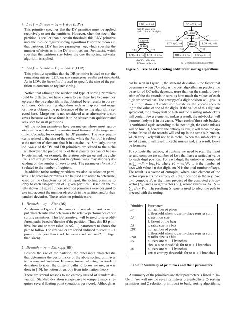
< S1<br />
LDR r=5, t=0<br />
(a) CC−radix <strong>with</strong><br />
radix 5 for all the digits<br />
DR r=8<br />
B Size<br />
LDR r=4, t=16 LDR r=8, t=16<br />
(b)CC− radix <strong>with</strong><br />
different radix sizes<br />
< V1<br />
DP s=32K, f=4<br />
B Entropy<br />
>=V1 && V2<br />
LDV np=2, t=8 B Size LDR r=8, t=16<br />
>= S1 < S1<br />
>=S1<br />
LDR r=8, t=16 LDV np=2, t=8<br />
(c) Composite sorting algorithm<br />
Figure 5: Tree based encoding of different sorting algorithms.<br />
can be seen in Figure 1, the standard deviation is the factor that<br />
determines when CC-radix is the best algorithm, in practice the<br />
behavior of CC-radix depends, more than on the standard deviation<br />
of the the records to sort, on how much the values of each<br />
digit are spread out. The entropy of a digit position will give us<br />
this information. CC-radix sort distributes the records according<br />
to the value of one of the digits. If the values of this digit are<br />
spread out, the entropy will be high and the resulting sub-buckets<br />
will contain fewer elements, and, as a result, the sub-bucket will<br />
be more likely to fit in the cache. When each of these sub-buckets<br />
is partitioned again according to the next digit, the cache misses<br />
will be low. If, however, the entropy is low, it will mean the opposite.<br />
Most of the records will end up in the same sub-bucket,<br />
which very likely will not fit in cache. When this sub-bucket is<br />
sorted again, it will result in cache misses and, as a result, lower<br />
performance.<br />
To compute the entropy, at runtime we need to scan the input<br />
set and compute the number of keys that have a particular value<br />
for each digit position. For each digit, the entropy is computed<br />
as ∑ i −P i ∗ log 2 P i , where P i = c i /N , c i is the number of<br />
keys <strong>with</strong> value i in that digit, and N is the total number of keys.<br />
The result is a vector of entropies, where each element of the<br />
vector represents the entropy of a digit position in the key. We<br />
then compute S, as the inner product of the computed entropy<br />
∑<br />
vector (E i ) and a weight vector (W i ), whose values we fix: S =<br />
i E i ∗ W i . The resulting S value is used to select the path to<br />
proceed <strong>with</strong> the sorting.<br />
Primitive<br />
DV<br />
DP<br />
DR<br />
LDV<br />
LDR<br />
BN<br />
BE<br />
Parameters<br />
np: number of pivots<br />
t: threshold when to use in-place register sort<br />
s: partition size<br />
f: fanout of the heap<br />
r: radix size is r bits<br />
np: number of pivots<br />
t: threshold when to use in-place register sort<br />
r: radix size is r bits<br />
n: there are n +1branches<br />
size: n size thresholds for to n +1branches<br />
n: there are n +1branches<br />
ent: n entropy thresholds for to n +1branches<br />
Table 1: Summary of primitives and their parameters.<br />
A summary of the primitives and their parameters is listed in Table<br />
1. We will use the seven primitives presented here (5 sorting<br />
primitives and 2 selection primitives) to build sorting algorithms.