Optimizing Sorting with Genetic Algorithms - Polaris

chine and the characteristics of the input data. The intuition behind
this is that different partitions of the input data benefit more from
different sorting algorithms and, as a result, the optimal sorting algorithm
should be the composition of these different sorting algorithms.
Beside the sorting primitives, the generated code contains
selection primitives that adapt at runtime to the characteristics of
the input. The search for the optimal composite sorting algorithm
is done using genetic algorithms [5]. Genetic algorithms have also
been used to search for the appropriate formula in SPIRAL [13]
and to optimize compiler heuristics [14].
Our results show that this approach is very effective. The best
composite algorithm we have been able to generate are up to 42%
faster than the best “pure” sorting algorithms.
The rest of this paper is organized as follows. Section 2 discusses
the primitives that we use to build sorting algorithms. Section
3 explain why we chose genetic algorithms for the search and
explains some details of the algorithm that we implemented. Section
4 shows performance results, and finally Section 5 presents the
conclusion.
2. SORTING PRIMITIVES
In this section, we describe the building blocks of our composite
sorting algorithms. These primitives were selected based on experiments
with different sorting algorithms and the study of the factors
that affect their performance. A summary of the results of these experiments
is presented in Figure 1 which plots the execution time
of three sorting algorithms against the standard deviation of the
keys to be sorted. Results are shown for two platforms, Intel Pentium
III Xeon and Sun Ultra-Sparc III, and for two data sets sizes
2M (figures on the left) and 16M (figures on the right). The three
algorithms are: quicksort [6, 12], a cache-conscious radix sort (CCradix)
[7], and multiway merge sort [9]. Figure 1 shows that for
2M records, the best sorting algorithm is either quicksort or CCradix.
However, for 16M records, multiway merge or CC-radix
are the best algorithms. The input characteristics that determine
when CC-radix is the best algorithm is the standard deviation of
the records to be sorted. CC-radix is better when the standard deviation
of the records if high, because if the values of the elements in
the input data are concentrated around some values, it is more likely
that most of these elements end up in a small number of buckets.
Thus, more partitions will have to be applied before the buckets fit
into the cache and therefore more cache misses are incurred during
the partitioning. On the other hand, if we compare the performance
on the two platforms we can see that, although the general trend of
the algorithms is always the same, the performance crossover point
occurs at different points.
Other experiments, not described in detail here, have shown that
the performance of the pure quicksort algorithm can be improved
when combined with other algorithms. For example, experimental
results show that when the partition is smaller than a certain
threshold (whose value depends on the target platform), it is better
to use insertion sort or register sort [10], instead of continuing
to recursively apply quicksort. Register sort is a straight-line code
algorithm that performs compare-and-swap of values stored in processor
registers [9]. The idea of using insertion sort to sort the small
partitions that appear after the recursive calls of quicksort was also
used in [12] to improve the performance of quicksort.
In this paper, we search for an optimal algorithm by building
composite sorting algorithms. This approach was also followed in
[3] to classify several sorting algorithms. We use two types of primitives:
sorting and selection primitives. Sorting primitives represent
a pure sorting algorithm that involves partitioning the data, such as
radix sort, merge sort and quicksort. Selection primitives represent
a process to be executed at runtime that dynamically decide which
sorting algorithm to apply.
The composite sorting algorithm we used in this study assumes
that the data is stored in consecutive memory locations. The data
is then recursively partitioned using one of three partitioning methods.
The recursive partitioning ends when a leaf sorting algorithm
is applied to the partition. We now describe the three partitioning
primitives followed by a description of the two leaf sorting primitives.
1. Divide − by − Value(DV)
This primitive corresponds to the first phase of quicksort which,
in the case of a binary partition, selects a pivot and reorganizes
the data so that the first part of the vector contains the keys with
values smaller than the pivot, then comes the pivot, and the third
part contains the rest of the keys. In our work, the DV primitive
can partition the set of records into two or more parts using a
parameter np, that specifies the number of pivots. Thus, this
primitive divide the input set in np +1partitions, and rearranges
the data around the np pivots.
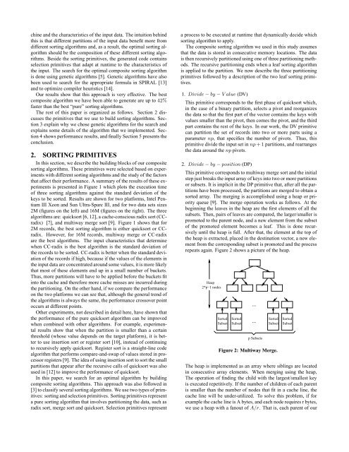
2. Divide − by − position (DP)
This primitive corresponds to multiway merge sort and the initial
step just breaks the input array of keys into two or more partitions
or subsets. It is implicit in the DP primitive that, after all the partitions
have been processed, the partitions are merged to obtain a
sorted array. The merging is accomplished using a heap or priority
queue [9]. The merge operation works as follows. At the
beginning the leaves in the heap are the first elements of all the
subsets. Then, pairs of leaves are compared, the larger/smaller is
promoted to the parent node, and a new element from the subset
of the promoted element becomes a leaf. This is done recursively
until the heap is full. After that, the element at the top of
the heap is extracted, placed in the destination vector, a new element
from the corresponding subset is promoted and the process
repeats again. Figure 2 shows a picture of the heap.
Heap
2*p−1 nodes
...
Sorted Sorted
Sorted Sorted
...
Subset Subset Subset Subset
p Subsets
Figure 2: Multiway Merge.
The heap is implemented as an array where siblings are located
in consecutive array elements. When merging using the heap,
The operation of finding the child with the largest/smallest key
is executed repetitively. If the number of children of each parent
is smaller than the number of nodes that fit in a cache line, the
cache line will be under-utilized. To solve this problem, if for
example the cache line is A bytes, and each node requires r bytes,
we use a heap with a fanout of A/r. That is, each parent of our