Preprint

Uniform asymptotics of Poisson approximation to thePoisson-binomial distributionHsien-Kuei Hwang, Vytas ZacharovasInstitute of Statistical ScienceAcademia SinicaTaipei 115TaiwanFebruary 12, 2008AbstractNew uniform asymptotic approximations with error bounds are derived for a generalized total variationdistance of Poisson approximations to the Poisson-binomial distribution. The method of proof isalso applicable to other Poisson approximation problems.MSC 2000 Subject Classifications: Primary 62E17; secondary 60C05.1 IntroductionWe study in this paper a fundamental problem in probability theory: how good is Poisson approximationto the Poisson-binomial distribution (of which binomial is a special case)? We re-examine this old andextensively studied problem and derive new estimates from a different viewpoint.1.1 Poisson approximation to binomial distributionWe start with the simplest case of a binomial distribution. Let Bi.nI p/ denote a binomial distribution ofparameters n and p, 0 < p < 1. Let Po./ denote a Poisson distribution with mean . It is well knownsince Siméon-Denis Poisson [23] that if np ! c < 1 then the binomial distribution Bi.nI p/ convergesto the Poisson distribution with mean c, as n ! 1 (he proved indeed an equivalent version for negativebinomial distribution). More than a century later, Prokhorov [24] extended Poisson’s limit theorem to anapproximation theorem and was the first to show that the total variation distanced TV .Bi.nI p/; Po.np// WD 1 Xˇ n2 ˇ p j .1 p/ n j ejsatisfies (see [5] for a minor correction)d TV .Bi.nI p/; Po.np// Dj0np.np/jj !p p 1 C O min.1; p C .np/ 1=2 / : (1.1)2eˇ1

This says that Poisson approximation to binomial distribution is good as long as p is small. Observe thatwhen np ! 1 the O-term in (1.1) is asymptotically smaller than the dominant term, while in the caseof bounded np, the right-hand side becomes an upper bound. Thus (1.1) extends Poisson’s original limittheorem in two directions: in degree of precision and in range of variations of p. Such an extension hassince attracted the interest of many probabilists and many powerful tools have been developed; see, inparticular, [4, 5, 8, 9, 16, 21, 27] and the references therein for more information.Second-order refinement. A natural question regarding the approximation (1.1) is that how good theleading term is. Or, is the error term optimal? This raises the question of second-order expansion inPoisson approximation problems, which, as far as we were aware, was first addressed by Kerstan in [18].His results implicitly imply that if p D o.1/, then ( WD np)whered TV .Bi.nI p/; Po.// D pT C O.p 2 /; (1.2)T WD 1 4Xj0 jj !ˇˇˇˇ e .j / 2 jNote that T D .2e/ 1=2 .1 C ‚. 1 //; see also [9, 15]. In particular, for p D o.1/ and ! 1,d TV .Bi.nI p/; Po.// D p p 1 C O p C 1 I (1.3)2ecompare (1.1). The asymptotic nature of Prokhorov’s result (1.1) is now clearer. Note that the minimumerror (of the O-term) is reached when p D 1 , or when p D n 1=2 . Kerstan’s result was later extendedin [2, 4, 8, 11, 27] by different approaches; see also the book [5] for more details.New uniform approximations.distanceˇ :Instead of the total variation distance, we consider in this paper thed .˛/TV .L.X /; L.Y // WD 1 2XjP.X D m/ P.Y D m/j˛ ; (1.4)mbetween the distributions of the two discrete random variables X and Y , where, here and throughout thispaper, ˛ > 0 is a fixed constant. The interest of considering d .˛/TV is multifold. First, such a quantityis, modulo power, the natural analogue of the usual `p-norm; see [25, Ch. 2] and [27]. When ˛ D 1the above quantity coincides with the usual total variation distance d TV . Second, it can be regarded as aneffective measure of robustness of Poisson approximation; see Corollary 1.4 and its discussions. Third,several approaches to Poisson approximation apply well only for special values of ˛ but not for all. Thus,its consideration also introduces more methodological interests. Indeed, most of our proofs will largelysimplify if we consider only the case when ˛ 1.Throughout this paper, q WD 1 p.Theorem 1.1. If p 1=2 and WD np ! 1, thend .˛/.1TV .Bi.nI p/; Po.// D p˛ ˛/=2J˛.p/where J˛.p/ is bounded for p 2 .0; 1/ and ˛ > 0, and defined by1J˛.p/ De ˛t 2 =2e pt 2 =.2q/p 12.2/˛=2 p˛ˇ q ˇZ 111 C O .˛C1/=2 C 1 ; (1.5)˛dt: (1.6)2

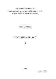
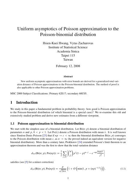
Note that if p > 1=2, we can interchange the role of p and q and the same approximation holds withappropriate changes of p and q.While less explicit, the approximation (1.9), especially the function J˛.p/, is seen to contain muchinformation. Roughly, we may say that most dependence on p of d .˛/TV is encapsulated into J˛.p/ (although itself depends on p). Also the smooth transition of d .˛/TV from p D o.1/ to p 2 Œ"; 1=2 is visible from(1.5). On the other hand, the uniformity provided by such an approximation is of practical value sincemost practical parameters are finite and it is often not easy to tell if a given small p is o.1/ or O.1/.For integer values of ˛, we have, by splitting the integral according to the sign of 1 e px2 =.2q/ = p qand then evaluating the corresponding integrals,J 2m .p/ DJ 2mC1 .p/ D1 X2.2/ m 1=2 p 2m12.2/ m p 2mC1 3 4ˆ0j2mX0j2mC1s 2mj 2m C 1. 1/ j q .j 1/=2 .2mq C pj / 1=2 .m 1/;j..2m C 1/q C pj / 1 p log 1 q. 1/ j q .j 1/=2 ..2m C 1/q C pj / 1=2!!; .m 0/;where ˆ.x/ WD .2/ 1=2 R x1 e t 2 =2 dt denotes the standard normal distribution function. In particular,s! s!!J 1 .p/ D 2 p ˆ 1p log 11 pˆ1 pp log 1; (1.7)1 pp p pq.1 C q/ 2 2q C 1 C qJ 2 .p/ D4 p p 2p :q.1 C q/For non-integral values of ˛, no simple explicit expressions are known for J˛. However, numericalcalculation does not pose any problem since the integrand decays exponentially fast for large parameter andp bounded away from 1; see Figure 1 for a plot of J 1 .p/ and J 1=2 .p/. Note that J 1 .0/ WD lim t!0 C J 1 .t/ D1= p 2e and J 1 .1/ WD lim t!1 J 1 .t/ D 1.In particular, taking ˛ D 1, we obtain the following refinement to (1.3).Corollary 1.2. If p 1=2 and ! 1, thend TV .Bi.nI p/; Po.// D pJ 1 .p/ 1 C O 1 : (1.8)The result (1.8) is to be compared with (1.3).On the other hand, J 0 1 .0/ D J 1.0/=2 D 1=.2 p 2e/; we thus haved TV .Bi.nI p/; Po.// Dp p2e1 C p 2 C O p2 C .np/ 1 ;as ! 1 and p D o.1/; compare (1.3). We see that the remainder term in the above formula is of orderrn 2, where r n D p C .np/ 1=2 , while the error term in the original Prokhorov’s result (1.1) is of order r n .The second uniform asymptotic approximation we derive to d .˛/TV .Bi.nI p/; Po.np// for small p is asfollows, which extends Kerstan’s (1.2); see also [27].3

J 1 .p/J 1=2 .p/1:01:30:81:20:61:10:40:20:2 0:4 0:6 0:8 1:0p10:90:2 0:4 0:6 0:8 1:0pFigure 1: The two functions J 1 .p/ and J 1=2 .p/ plotted against p. Note that as p grows, J 1=2 .p/ firstincreases and then suddenly decreases near unity. Such a behavior is typical for J˛.p/ when ˛ 2 .0; 1/.The reason is that when ˛ < 1 and p ! 1 the integral in (1.6) over e pt2=.2q/ = p q 1 is asymptoticto p =.2˛/ .1 p/ .1 ˛/=2 while the remaining integral is asymptotic to p =.2˛/. On the other hand,J˛.p/ ! 1 when ˛ > 1 and p ! 1 .Theorem 1.3. If p D o.1/ and K > 0, thend .˛/.1TV .Bi.nI p/; Po.np// D p˛ ˛/=2T˛./1 C O Kp C p˛ 1=2 ; (1.9)where T˛ is bounded for all and ˛ > 0 and given byT˛./ D1.2 p X/ 1C˛j0e jj !˛ˇˇ.j /2j ˇˇ˛ : (1.10)Like J˛, the series T˛ also contains much information. From a computational point of view, thefunction T˛ looks complicated and is not much simpler than directly computing the sum-definition ofd .˛/TV .Bi.nI p/; Po.np//. However, in the case of general Poisson-binomial and other distributions, a directcalculation of d .˛/TV is very messy and less tractable for large n. In such a case, it is useful to use (1.9)since T˛ is distribution-independent. Moreover, the calculation of T˛ does not introduce any problem inpractice because the terms in (1.10) converge factorially fast for small , while for large , one can usestraightforward Gaussian approximation with the desired error bounds.Note that the only case not covered by Theorems 1.1 and 1.3 is when p D o.n 1 / for which bothdistributions (binomial and Poisson) degenerate and the corresponding approximation problem has beenwell studied in the literature; see [9, 17].Robustness of Poisson approximation. From an approximation point of view, an immediate consequenceof the two uniform estimates (1.5) and (1.9) is as follows.Corollary 1.4. The distance d .˛/TV .Bi.nI p/; Po.np// tends to zero as n ! 1 if (i) ˛ > 1 or (ii) ˛ 1 andp D o.n .1 ˛/=.1C˛/ /.Thus Poisson approximation to binomial distribution is always good if ˛ > 1 (even when p is notsmall), or if p is suitably small when ˛ 1.4

On the other hand, another natural question is: which of the two approximations (1.5) and (1.9) is betterin the overlapping range (for numerical purposes) when all parameters are given? Roughly, we see that(1.5) is preferable for large while (1.9) is better for small . More precisely, if ˛ 1, then p D n 1=2is the threshold of choosing (1.5) or (1.9), namely, if p n 1=2 then use (1.5), otherwise use (1.9). Notethat in either case, the error term is of order n 1=2 in the worst case, in contrast to (1.3) for which the errorterm is n 1=2 in the best case.When ˛ 2 .0; 1/, then by comparing the two error terms n .˛C1/=2 and p C p˛ 1=2 , we see that thethreshold becomes p D n .˛C1/=.˛C3/ , namely, if p n .˛C1/=.˛C3/ , then the error term .˛C1/=2 issmaller than that in (1.9), while if p n .˛C1/=.˛C3/ , then the use of (1.9) yields a smaller error than thatof (1.5). In either case, the worst error is order n .˛C1/=.˛C3/ .1.2 Poisson approximation to the Poisson-binomial distributionSimilar results as above can be obtained for the Poisson-binomial distribution. In this case, we haveS n WD X 1 C X 2 C C X n , where the X j ’s are independent Bernoulli random variables withP.X j D 1/ D 1 P.X j D 0/ D p j :Let k D P 1jn pk j for k 1. With this notation, we have E.S n/ D 1 and V.S n / D 1 2 . Forconvenience, we write D 1 . Let WD 2 =.Theorem 1.5. If 1=2 and ! 1, thend .˛/TV .L.S .1n/; Po.// D ˛ ˛/=2J˛./ 1 C O .˛C1/=2 C 1 ;where J˛ is defined in (1.6).Note that Theorem 1.1 is a special case of Theorem 1.5, and here plays the role of p.Theorem 1.6. If D o.1/ and K > 0, thend .˛/TV .L.S .1n/; Po.// D ˛ ˛/=2where T˛ is defined in (1.10) and WD C 3 =. 2p/.T˛./1 C O K C ˛ 1=2 :Note that the quantity becomes p C p 1=2 when p j D p for all j D 1; : : : ; n. Also the O-termtends to zero when ! 0 and ! 1; it is also infinitesimally small when ! 0 and K > 0because 3 =. 2p/ p2 = D p .The results of both theorems are new except for Theorem 1.6 in the special case when ˛ 1, whichis covered by Theorem 3 in Roos (1999). For earlier results for ˛ D 1 (with weaker error bounds),see [8, 12, 13, 18]; the optimal error term was first derived in [4] by improving the Stein-Chen method.Effectiveness of both results can be addressed as in the binomial case and is not given here (indeed allresults there hold by replacing p by ).1.3 Methods of proof and organization of the paperThe tools we developed are based on Fourier analysis with several new ingredients. They are general andapplicable to many other metrics. A brief discussion of the Kolmogorov distance and the point metric isgiven in Section 2.10. The main ideas of our proofs consist in deriving a few precise local limit theorems5

(LLTs) for S n , with a more careful control of the error bounds (LLTs in the usual form or with largedeviations being insufficient for our uses). Then we decompose the sum in (1.4) into major and minorparts, and evaluate the contribution of each. The idea is straightforward, but the technicalities, especiallythe error analysis, are more delicate and highly nontrivial.The approach we used is also applicable to many other Poisson and non-Poisson approximation problems.A large number of examples and extensions can be found in [15]; for many others, see for example[5].Poisson approximation has received extensive attention in recent probability and applied probabilityliterature, and several different approaches have been proposed; see, for example, [1, 3, 5, 15, 20, 22, 28,30] and the references therein.This paper is organized as follows. To prove Theorems 1.5 and 1.6, we first establish another (more)uniform approximation to d .˛/TV from which both theorems will follow. Although Theorems 1.1 and 1.3 arespecial cases of Theorems 1.5 and 1.6, respectively, we will sketch an elementary approach in Appendixfor more methodological interests.Notation. Except for the parameter whose use is clear in each occurrence, the use of all other symbolswill be kept consistent.2 A more uniform approximation to d .˛/TV .L.S n/; Po.//Although the ranges specified by the two main approximation theorems 1.5 and 1.6 differ, their formssuggest the possibility of an asymptotic approximation holding uniformly in an even wider range than thatcovered by both theorems, which is the aim of this section. Indeed, the proof of the two main approximationtheorems 1.5 and 1.6 relies on the following result, which is more uniform but at the price of a morecomplicated sum-approximant.Throughout this section, WD p 2 .Theorem 2.1. Let x D x m WD .md .˛/TV .L.S n/; Po.// D W˛.//=. If 1=2 and K > 0, then 1 C O K˛1 ˛ 1=2 C 1 1 ;where 1 WD C 3 = 2 ,W˛./ WD 1 X2m0e me x2 =2˛pm!ˇˇˇˇˇ 11 C C 1x C C 2 x 3 1ˇ˛; (2.1)the two constants C 1 ; C 2 being bounded for all p j ’s defined byC 1 WD . 2 2 3 / C 2 22 2 and C 2 WD 2 3 2 3 2 2 C 3 26 2 2 : (2.2)Since W˛./ is a function of and , we can derive more precise expansions when is large or when is small. More precisely, if is large, then the sum W˛ can be approximated by an integral with the useof the LLT for Poisson distribution. This will prove Theorem 1.5. On the other hand, if is small, then wecan expand the terms inside the absolute-value sign in (2.1) with respect to and then deduce the estimateof Theorem 1.6.6

To prove Theorem 2.1, let ı n;m WD P.S n D m/ e m =m!, andF.z/ WDXP.S n D m/z m DY.q j C p j z/ D Y.1 C p j .z 1//;0mn1jn1jnwhere q j WD 1 p j . We first derive estimates for jı n;m j, k and jF.z/j. Then we prove several differentversions of LLTs for S n , from which Theorem 2.1 will be deduced.2.1 An estimate for Poisson distributionWe start with an inequality for the Poisson distribution that will be used later. It is taken from [5, p. 259].Lemma 2.2. For m 1e mm! e .m /2 =.2.mC//p2 m: (2.3)Proof. A direct proof is as follows. By the inequality m! p 2 m.m=e/ m , we havee mm! 1p exp2 m 1m C m log m :Then the upper bound (2.3) will follow from the elementary inequality 1 xCx log x .1 x/ 2 =.2.1Cx//for x > 0, or, equivalently,Z x0log.1 C t/dt x 22.2 C x/.x > 1/: (2.4)To prove (2.4), observe first that log.1 C t/ t=.1 C t/ for t > 1 since R tRlog.1 C v/dv 0. Then0 x log.1 C t/dt R xt=.1 C t/ dt, and the right-hand side is bounded below by 0 0 x2 =.2.2 C x// byconsidering the two cases x 0 and x 2 . 1; 0.2.2 A crude estimate for jı n;m jLemma 2.3. For m 1, we havewhere c 1 WD e 2 =2.Proof. First, by partial summation,0e .z 1/ F.z/ D X1jnD X1jnjı n;m j c 1 21 C .m=/ 2 e .m /2 =.2.mC// ; (2.5)@e .p j CCp n /.z 1/Y1`

from this and the elementary inequalitiesj1 C p.z 1/j 1 p C pjzj D 1 C p.jzj 1/ e p.jzj 1/ .p 2 Œ0; 1/;ˇZ 1ˇez 1 zˇˇ D ˇˇz2 e tz .1 t/dtˇ jzj22 ejzj ;0we obtainjF.z/ e .z 1/ j X1jne .jzj1/ P`6Dj ˇp` ˇep j .z 1/ c 1 2 e .jzj 1/ jz 1j 2 :Substituting this bound in the Cauchy integral formula, we get1 p j .z 1/ˇˇfor any r > 0. Taking r D m= givesjı n;m j c 1 2 min r m e .r 1/ .1 C r 2 /;r>0jı n;m j c 1 21 C .m=/ 2 e m m log.m=/ c 1 21 C .m=/ 2 e .m /2 =.2.mC// ;where the last estimate is obtained by the same proof of Lemma 2.2. This proves the Lemma.2.3 Estimates for quantities involving kWe prove in this subsection a few estimates for k and k .r/ defined as follows. Let r WD 1 C x=, wherex WD .m /=. (Recall that D p 2 .) Then k .r/ WD Xp j .r/ k ; p j .r/ WD p jrq j C p j r :1jnThe reason of introducing the k .r/’s is because the usual LLT is not sufficient for our purpose and wewill need LLTs for moderate and large deviations. More precisely, define the Bernoulli random variablesX j .r/ such thatP.X j .r/ D 1/ D 1 P.X j .r/ D 0/ D p j .r/:Let S n .r/ WD X 1 .r/ C C X n .r/. Then S n and S n .r/ are connected by the relationbecause (q j .r/ D 1p j .r/)F.rI z/ WDLemma 2.4. For any > 0,Y1jnP.S n D m/ D r m F.r/ P.S n .r/ D m/; (2.6).q j .r/ C p j .r/z/ D X0mnP.S n .r/ D m/z m D F.rz/F.r/ :0 1 ./ k ./ maxf; 1 g.k 1/ 2 .k 1/; (2.7)and 1 ./ 2 . 2/: (2.8)8

Proof. The upper bound of (2.7) follows immediately fromsince0 1 ./ k ./ D X .k1jn " p j11 C . 1/p j1/ XIn particular, when D 1, (2.7) has the formFor (2.8), we have 1 ./ D X 1 21jnp jp 2 j11 C . 1/p j 2 #1 p k 1j1 C . 1/p j.minf1; g/ 2 .k 1/ 2 ;1 C . 1/p j D q j C p j minf1; g: (2.9)1jnX1jnp j 10 k .k 1/ 2 : (2.10)p j X1 C . 1/p jp j 1 2X1jnp j 11jnp j 1p j 1 C . 1/p jp j .1 p j / D 2 . 2/:Lemma 2.5. For r D 1 C x=,.r 1/20 m 1 .r/ . 2 3 /minf1; rg ; (2.11)and, if x D o./ as ! 1, then1p1 .r/ 2 .r/ D 1 Proof. We have1 3 2 C 2 32 3x C O x2 2 : (2.12) 1 .r/ 2 .r/ D r X p j pj2.1 C .r 1/p j / 21jnD r 2 1 2 2 3 3 4x C O 3 4x 2 ;which, together with the estimate r 1=2 D 1 x=.2/ C O x 2 = 2 , yields (2.12). Note that the factor. 3 2 C 2 3 /= 3 is of order 1 .Similarly, since m D C.r 1/ 2 , we have m 1 .r/ D .r 1/ P 2 1jn p2 j .1 p j/=.1C.r 1/p j /,from which (2.11) follows.9

2.4 Estimates for jF.z/j and jF.rI z/jSince our approach is based on Cauchy’s integral formula, we also need some estimates for the probabilitygenerating functions F.z/ and F.rI z/.Let .r/ WD p 1 .r/ 2 .r/.Lemma 2.6. .i/ For jxj 1=3 with 2,.ii/ For jtj ,F.r/r D e x2 =21 C 3 2 C 2 3x 3 C Om 6 3 1 C x6 2: (2.13)jF.rI e it /j e c 2.r/ 2 t 2 ; (2.14)where c 2 WD 2= 2 ..iii/ For jtj 2=3 and jxj 1=3 with 2,F.rI e it /e mit D e .r/2 t 2 =21 C . 1 .r/ m/i tC 1.r/ 3 2 .r/ C 2 3 .r/.i t/ 3 C O.x 4 t 2 C 4 t 6 C 2 t 4 / : (2.15)6Proof. Since r D 1 C x=, 2 and jxj 1=3 , we see that jr1j 2 1=6 < 1, and thuslog F.r/r mD X j1D. 1/ j 1 . j m/.r 1/ jjx22 C 3 2 C 2 3x 3 C O6 3 x4 2 ;because, by (2.10), j m D j x D O j 2 for j 1. This proves (2.13).For (ii), we start from the relationjq C pe it j 2 D q 2 C p 2 C 2pq cos t D 1 2pq.1 cos t/ .t 2 R/;which yields the inequality jq C pe it j 2 e 2pq.1 cos t/ . This and the inequality 1 cos t c 2 t 2 forjtj giveˇYˇF.rI e it /ˇˇ D jq j .r/ C p j .r/e it j e .r/2 .1 cos t/ e c 2.r/ 2 t 2 ;1jnfrom which (2.14) follows.Finally, for (iii), by Taylor expansion and (2.10), we havelog F.rI e it /e mit D . 1 .r/m/i t C X . 1/ k 1. k .r/ 1 .r//.e it 1/ kkk2D . 1 .r/m/i t.r/ 2t 2 C 1.r/23 2 .r/ C 2 3 .r/6.i t/ 3 C O 2 t 4 :This proves (2.15) and the lemma.10

2.5 The usual LLT for S nWith the above estimates available, we can now prove four LLTs, starting from the one in the usual form.Proposition 2.7. If ! 1 as n ! 1; thenP.S n D m/ D e x2 =2p2 1 C 3 2 C 2 36 3 .x 3 3x/ C Ouniformly for m D C x with jxj 1=3 . x 6 C 1 2: (2.16)Proof. By Cauchy’s (or Fourier’s) integral formulaP.S n .r/ D m/ D 1 Ze mit F.rI e it /dt C 1 Ze mit F.rI e it /dt2 jtjt 02 t 0

2.6 A refined LLT for S nThe error term of the LLT (2.16) is insufficient for our purpose. We derive a crucial LLT with a better errorterm in this subsection. Let … m ./ WD e m =m! and define the k-th difference operatorZ k … m ./ WD 1 e mitC.ei t 1/ .1 e it / k dt2D … m ./ X kjm.m 1/ .m j C 1/. 1/ .k D 0; 1; : : : /: (2.19)j j0jkProposition 2.8. If thep j ’s satisfy 2 = 1=2 and c, where c > 0 is an arbitrary fixed constant,then uniformly for m 0P.S n D m/ … m ./ D 22 2 … m ./ C 33 3 … m ./ C I C O 4 5=2 C 2 3=2 ; (2.20)where the implied constant in the O-symbol depends only on c andI WD 1 Z 1e . m/it t 2 =21 C 2 16 .i t/3 .t/dt;with.t/ WD e 2t 2 =2For results similar to (2.20), see [7, 19].1 22 t 2 22Proof. Assume first that max 1jn p j 1=10. Then k 10 1ˇˇlog.1 C z/ zC z22z 33ˇ 3.i t/ 3 e 2t 2 =23jzj 44.1 jzj/1 : (2.21)k for k 2. By the expansion.jzj < 1/;we have, with some function c.t/ satisfying jc.t/j 1=2 for jtj ,F.e it / e .ei t 1/ D e .ei t 1/e 2.e i t 1/ 2 =2C 3 .e i t 1/ 3 =3Cc.t/ 4 je i t 1j 4 1D e .ei t 1/E.t/ C O . 4 t 4 C 2 3 t 6 /e c 3 2 t 2 ; (2.22)where we can take c 3 D 3=5 and E.t/ WD e 2.e i t 1/ 2 =2 1 C 3 .e it 1/ 3 =3 1. NowE.t/ C 22 .eit 1/ 2 33 .eit 1/ 3D e 2.e i t 1/ 2 =21 C 22 .eit 1/ 2C 33 .eit 1/ 3 e 2.e i t 1/ 2 =21 C 22 .eit 1/ 2 2 36 .eit 1/ 5 :By the inequality j.e it 1/ 2 .i t/ 2 j jtj 3 , we have the expansione 2.e i t 1/ 2 =2 D e 2t 2 =2 212 .eit 1/ 2 .i t/ 2 C O 2 t 6 e 2t 2 =2:12

It follows thatE.t/ C 22 .eit 1/ 2 33 .eit 1/ 3D e 2t 2 =2 212 Œ.eit 1/ 2 .i t/ 2 C 33 .i t/3 e 2.it/ 2 =21 C 2C OD e 2t 2 =2 2 2 3 t 8 e 2t 2 =2 C 2 2 t 6 e 2t 2 =2 212 t 2 21C 33 .i t/3 e 2t 2 =21 C O1 C 22 .eit 1/ 22 .i 2 3t/2 .i t/5612 .i t/2 C .i t/ 3 e 2t 2 =2 2 2 3t 8 e t 2 2 =2 C 2 2 t 6 e t 2 2 =2ThusE.t/ D 22 .eit 1/ 2 C 33 .eit 1/ 3 C .t/ C O 2 2 3t 8 e t 2 2 =2 C 2 2 t 6 e t 2 2 =2:Substituting this expression into (2.22), we then obtain, by Cauchy’s integral representation,:P.S n D m/e mm! D 22 2 … m ./ C 33 3 … m ./C 1 e mitC.ei t 1/ .t/dt C O2Z 4 5=2 C 2 3=2 :We now simplify the integral involving .t/. Since .t/ D O 2 2 t 4 e 2t 2 =2; (2.23)we have, for a suitably small " > 0,Z e mitC.ei t1/ .t/dt DZ "e . m/it t 2 =2"D 2I C O 2 3=2 :1 C 6 .i t/3 C O.t 4 C 2 t 6 / .t/ dt C O 2 3=2To complete the proof, we consider now the case when max 1jn fp j g 1=10. In this case, we splitthe integral into two partsP.S n D m/ e mm! D 1 Z 1=10 Z !Ce mit F.e it / e .ei t 1/dt:2 1=10 1=10

2.7 A simpler version of the refined LLTAlthough the integral I in (2.20) can be computed explicitly, the resulting expression is rather complicatedand not needed in this paper. We derive instead a simpler LLT at the price of weaker error terms; this LLTis also crucial in the development of our argument.Proposition 2.9. If 2 = D 1=2 and c > 0, thenP.S n D m/e mm! D 22 2 … m ./ C p 1 1p 12 1 2 .jm j 2 C 1/C OC 3.jm j C 1/ 3=2 5=2uniformly for m 0. The constant in the O-symbol depends only on c.2; (2.24)This expansion is useful when jmj is not too large.Proof. First, by (2.19), 3 … m ./ D Oe mm! 1 C jmj 2 Cjm j3: 3It remains, by (2.20), to simplify the integral I .I D 1 Z (1e t 2 =22 1 e 2t 2 =211 C . m/i t C O . m/ 2 t 2 1 C 22 t 2 223.i t/ 3 e 2t 2 =23.i t/33!1 ) dt:It follows, by expanding the factors inside the curly braces and by estimating term by term, thatI D 1 Z 1e t 2 =2e 2t 2 =2 212 12 t 2 dt Z 1C O j mj e t 2 =2 t 4 e 2t 2 =2 211 2 t 2 dtZ 1 C 2 j mj e t 2 =2 t 4 e 2t 2 =21 dt C 2 2 .j mj2 C 1/1 !7=2D p 1 1 2 2 .jm j 2 C 1/p 1 C O;2 1 2 = 2 3=2since the integrals involving odd integrands are equal to zero. This proves (2.24).2.8 Yet another LLT when 1=2We now derive another LLT for S n when D 2 = 1=2. This LLT is based on Proposition 2.8, and canbe regarded as a hybrid of Propositions 2.7 and 2.8.14

Proposition 2.10. Assume K > 0 and that m D C x satisfiesThen for 1=2P.S n D m/ D e m e x2 =2m! p 1 where C 1 , C 2 are given in (2.2).jxj C jxj3mD O 1=4 1=6 1 C C 1x C C 2 x 3and m 2 2 : (2.25) 2C O K C 431 C x2.1 C x /!!6 ; 2 m(2.26)Propositions 2.7 and 2.10 provide asymptotic approximations to the probability P.S n D m/ when mlies in the range 1=3 < m < 1=3 ;as ! 1. Proposition 2.7 can be used to estimate the closeness between P.S n D m/ and the densityof the normal distribution when " > 0, while proposition 2.10 yields a more accurate estimate when D o.1/.Proof. Since the range (2.25) is wider than that specified by the usual LLT (x D O.1/ or x D o. 1=6 /; see(2.16)) when ! 0, our method of proof here is to apply Proposition 2.8 to p j .r/ instead of to p j , whichgives an LLT for S n .r/, and then to use the relationship (2.6) between S n and S n .r/ to deduce (2.26). Asthe proof of Proposition 2.8, the error analysis constitutes the hard part of the proof.In what follows, we assume that ! 0, for otherwise (2.26) follows directly from Proposition 2.7.Smallness of 2 .r/= 1 .r/ 1=2 when ! 0. We first show that the probabilities p j .r/ satisfy thecondition of Proposition 2.8, namely, 2 .r/= 1 .r/ 1=2 when ! 0. To this purpose, we observe, by(2.9), that, for any > 0, k ./ maxf1; k g k .k 1/: (2.27)This (with k D 2) and the lower bound for 1 .r/ given in (2.8) yield 2 .r/r; 1 .r/ 2 max 1 2 2 r C 1 r r 2 r 2:r 2(2.28)Note that r can be expressed in terms of m as r D .m 2 /= 2 . From this, the condition m 2 2 , and 2 = ! 0, it follows that r C 1=r D m= C =m D O.1 C x 2 =m/. Consequently, by condition (2.25),we obtainjr 1j r C 1 D Ojxj 1 C jxj3 D O 1=4 1=3 I (2.29)rmthis estimate will be used several times below. In particular, this implies, by (2.28), that 2 .r/ 1 .r/ D O 2r C 1 D O. 3=4 / D o.1/; (2.30) r(by considering the two cases jxj 1=6 and jxj > 1=6 ).15

Application of Proposition 2.8 and simplification. From (2.30), we see that the probabilities p j .r/satisfy the condition of the Proposition 2.8, which, together with the two estimates,e 1.r/ 1.r/ mm!1 2 m m.m 1/C 1 .r/ 1 .r/ 2D O. 1 .r/ 1=2 /; (2.31)D 1 jm 1 .r/ C O 1 .r/j 2 C jm 1 .r/j; 1 .r/ 2(see (2.19)) for m 0, implies that P.S n .r/ D m/ D Q 1 C O.E 2 /, whereQ 1 WD e 1.r/ 1.r/ m1 C 2.r/ 11C p pm! 2 1 .r/ 21 .r/ 1 2 .r/= 1 .r/2 .r/E 2 WD 1 .r/1! 2 .r/;2 1 .r/ 2jm 1 .r/j 2 C 1 1 .r/ 3=2 C 2.r/.jm 1 .r/j C jm 1 .r/j 2 / C 3 .r/ 1 .r/ 5=2 : (2.32)Now from (2.11) and (2.29) it follows thatjm 1 .r/j D Ox1 2 C x2m.m 0/: (2.33)By substituting this, (2.27), and (2.30) into (2.32), we deduce that E 2 D O.E 3 /, whereE 3 WD 3=2 2 C 431 C x2.1 C x 4 /: mOn the other hand, by the estimatewe havee 1.r/ 1.r/ mm! 1jmp21 .r/ D O 1 .r/j 2 C 1 1 .r/ 3=2.m 0/;Q 1 D e 1.r/ 1.r/ m 1jm pm! 1 2 .r/= 1 .r/ C O 1 .r/j 2 C 1; 1 .r/ 3=2where the O-term is also bounded above by E 3 . Thus we obtainFurther simplification.haveP.S n .r/ D m/ D e 1.r/ 1.r/ m 1 pm! 1 2 .r/= 1 .r/ C O.E 3/: (2.34)Consider first the dominant term on the right-hand side of (2.34). By (2.33), we.m 1 .r// 2mD O 22! x4 1 C x2D O. 1=3 / D o.1/: (2.35)mThuse 1.r/ 1.r/ mm!D 1 mm! eD 1 mm! e mexp m log 1m m 21 C O x4 1 C x2m 1 .r/C mm 2!! 1.r/m: (2.36)16

Note that by (2.35) the terms inside the curly braces are bounded.Next we express the factor .1 2 .r/= 1 .r// 1=2 in terms of the j ’s. By straightforward expansion1p1 2 .r/= 1 .r/ D 1p1 1 C C 1x C Owhere C 1 is given in (2.2). Substituting this and (2.36) into (2.34), we obtainP.S n .r/ D m/ D.m=e/mm! p 1 2 C 3!!31 C x2; mx21 C C 1xC O.E 3 /; (2.37)where the new error terms introduced for the dominant term in (2.34) are absorbed in E 3 .Connection between the distribution of S n .r/ and that of S n . We now use (2.6) to derive (2.26).Consider F.r/. By Taylor expansionlog F.r/ D .r 1/ 22 .r 1/2 C 33 .r 1/3 C O .r 1/ 4 4:minf1; rgThe O-term is, by (2.25) and (2.29), of order O. 3=4 1=3 / D o.1/. Thus, similar to (2.36),becauseF.r/r m .m=e/mm! D e mr mm! F.r/e .r 1/ e rmD e mm! exp 22 .r 1/2 C 33 .r 1/3 C 1 C Or/4 ; .r 1/ 4 4minf1; rg C .mm 3m.m r/22mC .m r/33m 2m D r 2 .r 1/ (2.38)and .m r/ 4 =m 3 D O 4 2 .r 1/4 3 .r C 1=r/ 4 D o.1/. Hence by (2.38) and the conditions (2.25)on m, we can simplify the above estimate and obtainF.r/r m .m=e/mm!D e mm! e x2 =2x1 3C C 2 C O.E 4/ ;where C 2 is given in (2.2) and E 4 D x 4 1 2 C 3 = .1 C x 2 /. This also implies in particular thatF.r/=.r mp m/ D O e m e x2 =2 =m! . Combining this with (2.6) and (2.37), we deduce thatP.S n D m/ D e m e x2 =21m! p C C 1x C C 2 x 31 C O.E 5 / ;where E 5 WD 1=2 E 3 C E 4 . It is easily checked term by term that E 5 is bounded by the O-term on theright-hand side of (2.26). This completes the proof of the theorem.17

2.9 Proof of Theorem 2.1We are now ready to prove Theorem 2.1. The idea of proof is to split the sum P m0 jı n;mj˛ into twoparts according to m < 2 2 and m 2 2 . The former is easily estimated by applying Lemma 2.3 and isasymptotically negligible, while the latter is more involved and requires the more precise expansion (2.26).An estimate for P m

for sufficiently small , where c 4 and c 5 are positive absolute constants.Now for jxj 4 p 1 C 1=.4K/, we have ' 0 .x/ D 2.x x 0 / C O. 1 1=2 /, where x 0 WD 1=.2 p /;integrating this estimate, we obtain'.x/ D '.x 0 / .x x 0 / 2 C O. 1 1=2 / 3 4 C O. 1 1=2 /for jxfor jxx 0 j 1=2, and1 C O. 1 1=2 / j' 0 .x/j D O.1/; (2.44)x 0 j jxj 4 p 1 C 1=.4K/. Furthermore, it is easily checked thatr !' x 0 ˙ 2 1 C 1 1 C O. 1 1=2 /:4KFrom these estimates, we conclude that '.x/ has two zeroes x C D x C .; 2 ; 3 / and x D x .; 2 ; 3 /in the interval jxj 4 p 1 C 1=.4K/, such thatrx˙ ! ˙ WD x 0 ˙ 1 C 14 ; (2.45)uniformly for all K > 0 as ! 0.Since '.x C / D 0, we can integrate the estimate (2.44) and obtainZ xj'.x/j Dˇ ' 0 .t/ dtˇ jx C xj.1 C O. 1 1=2 //: (2.46)x CConsequently, there can be at most a finite number of m (indeed two if is sufficiently small) such thatj'.x/j 1 = and in that casejı n;m j˛˛ eˇˇˇe m '.x/=2m!ˇ1ˇ˛ D OOn the other hand, when j'.x/j 1 = and x satisfies (2.40), we havejı n;m j˛DD O˛ eˇˇˇe m '.x/=2m!˛ eˇˇˇe m '.x/=2m!˛ eˇˇˇe m '.x/=2Combining (2.47) and (2.48), we obtainXX ˛jı n;m j˛ De m '.x/=2ˇˇˇem!jxj.= 1 / 1=18 jxj.= 1 / 1=18m!C O 1D 2W˛./ C OXj'.x/j 1 = ˛˛1 3˛=2 : (2.47)ˇ1ˇ˛ ˇ1 .1 C x1ˇ˛10 ˛/1 C O1ˇ je '.x/=2 1j ˇˇ1ˇ˛ 1 1 .1 C x10 / : (2.48)ˇ1ˇ˛˛ eˇˇˇe m '.x/=2m! ˛1 .˛C1/=2 C ˛˛1 3˛=2 ;19! ˇ1ˇ˛ 1 C O ˛˛1 3˛=2

where W˛./ is defined in (2.1).The sum of jı n;m j˛ over the remaining range of m, namely, jxj .= 1 / 1=18 can be estimated bymeans of Lemma 2.2 and we obtainX ˛˛1 3˛=2 :jxj>.= 1 / 1=18 jı n;m j˛ D OLower and upper bounds for W˛./. To finish the proof, we need to estimate the order of W˛./. First,since C 1 D O./ and C 2 D O./, we have the upper bound01W˛./ D O @ X ˛ e ˛ m.1 C jxj 3 /˛ A D O ˛.1 ˛/=2 :m!m0Next, we see that the same estimate holds from below sinceW˛./ 1 X˛ eˇˇˇˇ m '.x/2m! 2 ˇjx x 0 j1=2 ˇˇ 3 ˛ 18ˇ2 C o.1/ Xjx x 0 j1=20 OX˛=2 @ ˛jxx 0 j1=2e ˛x2 .1˛˛ e m/=2as ! 0 and ! 1. This completes the proof of Theorem 2.1.2.10 Kolmogorov distance and the point metricm!1A O ˛ .1 ˛/=2 ;The methods of proof we used above can be readily amended for the consideration of other distances. Webriefly discuss the Kolmogorov distance and the point metric and start with the following lemma.Lemma 2.11. For m D C x 0P.S n m/P.S n D m/XjmProof. First of all, sincee jj ! D p22 1 … m ./ C ˆ 1C O p 1 ˆ.x/2 p 2 xe .1 /x2 =2 3 3=2 C 2 1=2 ; (2.49)e mm! D 22 2 … m ./ C e .1 /x2 =2p2 x2 .1 /x2 1 !1 C e x2 =2p1 C O 3 2 C 2 1 : (2.50)P.S n m/Xjme jj ! D 1 Z e mit F.eit / e .ei t 1/dt;2 1 e it20

we can apply the same proof used for (2.20) (Proposition 2.8), together with the expansionsand (2.22), and deduce thatP.S n m/Xjmwhere (.t/ is given in (2.21))1D 11 e it i t C 1 2 C O.jtj/;e jj ! D 22 1 … m ./ C 33 2 … m ./ C I 3 C O 4 2 C 2 1 ;I 3 WD 12Z 1e . m/it t 2 =21 C i16 .i t/3 t C 1 .t/ dtI2compare Theorem 1 in [29]. By the O-estimate (2.23) of .t/, we can simplify I 3 as follows.Z 11I 3 Di e . m/it t 2 =2 .t/dt C O 2 1=22tDi Z 1e . m/it t 2 =2e 2t 2 =2 2 dt12 12 t 2 C O 2 1=2t m m D ˆ p ˆ p C 2.m / 2 2 3=2p 2 e .m /2 =.2/ C O 2 1=2 :On the other hand, 2 … m ./ D O. 3=2 /. Collecting these estimates, we obtain (2.49).Similarly, we can show that 2 .; m/ and 3 .; m/ are smaller in order than the error terms ofthe estimates (2.49) and (2.50), respectively. Then (2.50) follows by the same line of arguments using theexpressionZ1 1p e yit t 2 =22 1e 2t 2 =21 22 t 2 dt D e y2 =.2 2 2 /p 2C e y2 =.2/2 5=2 . 2 2 2 C 2 y 2 /:We now derive asymptotic approximations to the Kolmogorov distance and the point metric betweenthe distribution of S n and Po./.Theorem 2.12. If ! 1 and 1=2, thensupˇˇP.S Xn m/ e jm0j !jm ˇ D 2 J 1./sup ˇˇP.S n D m/ e mm! ˇ D p 1 1 p 11 C O2 1 m0where J 1 is defined in (1.7).1 C O 1=2 ; (2.51) 1=2 ; (2.52)Proof. We first prove (2.51). By the usual LLT for Poisson distribution (2.18), we have, for m D C x,jxj 1=6 , 1 … m ./ D e m mp 1 1 D p xe .1 /x2 =2 1 C jxj31 C O p :m! 2 21

Substituting this estimate into (2.49), we obtainP.S n m/Xjme jj ! D ˆ p1 xˆ.x/ C O 1=2 ;for jxj 1=6 . ThussupˇˇP.S n m/m0Xjme jj !ˇ D1 C O 1=2ˇpsup ˇˆ 1x2R xˆ .x/ ˇ :Now it is straightforward to show that the maximum of the function jˆ. p 1 x/ ˆ.x/j is reached atx D ˙p 1 log.1 / (see also [31]). This proves (2.51).We now prove (2.52). First, by the usual LLT (2.18) and (2.19) with k D 2, we have, for m D C x,jxj 1=6 , 2 … m ./ D e .1 /x2 =2p2 .1 / 2 x 2 1 C OThis, together with the estimate (2.50), gives!P.S n D m/ e mm! D e .1 /x2 =2e x2 =2p p 12 1 1 C jxj3p :C O 1 :Then we deduce thatsup ˇˇP.S n D m/ e mm0m! ˇ D p 1sup e .1 /x2 =2e x2 =2p 12 x2R ˇ 1 ˇ C O 1 :Since the function x 7! e .1 /x2 =21 C e x2 =2 = p 1 reaches extrema at the points x D 0 andx D ˙p .3=/ log.1 /. Thuse .1 /x2 =2e x2 =2p 1ˇ 1 ˇ D max 1p 1;1 supx2RThis proves (2.52) and completes the proof of the theorem.D.1 / 3.1 /=.2/1p1 1:For more results on both distances, see [6, 10, 26, 27, 32] and the references cited there.3 Proof of Theorems 1.5 and 1.6The proof of Theorems 1.5 and 1.6 relies on Theorem 2.1 and Proposition 2.7. We prove first Theorem 1.6since its proof is shorter.Proof of Theorem 1.6. We start with the asymptotic estimate of d .˛/TV .L.S n/; Po.// provided by Theorem2.1. First of all, since D o.1/, by (2.42),e x2 =2p 1 C C 1x C C 2 x 31 1 D 2x 2 x p 1 C O .1 C x 4 / D 2 .x C/.x / 1 C O22.1 C x 4 /jx C jjx j;

uniformly for x bounded away from the two zeros ˙ WD .1 ˙ p1C 4/=.2 p / of the polynomialx 2 x= p 1; see (2.45). Obviously, the two zeros are bounded whenever ". Also, C > 0, < 0,and C > 2. Thus, by applying the estimate j1 C O.jtj/j˛ 1 D O.jtj/ for jtj 1, we obtainE 6 WD X ˛e me x2 =2p 1 C C 1x C C 2 x 31ˇm! ˇm01 ˇ˛ ˇˇˇˇ x 2 x˛!p21ˇˇˇˇD O ˛X˛ e mX˛!j.x C /.x /j˛ 1 .1 C x 4 / C e ˛˛ m;m!m!jxj 1=2jx ˙j>where jx ˙j > represents the two inequalities jx C j > and jx j > . For the first sum in theO-symbol, we use (2.3) and deduce thatX˛e mj.x C /.x /j˛ 1 .1 C x 4 / D O ˛=2 .˛ 1 C 1=2 / Im!jxj 1=2jx ˙j>similarly, by the crude bound (2.31), we see that the second sum in the O-symbol of (3.1) satisfiesX˛e mD O1 ˛=2 C 1=2 :m!ThusThis completes the proof.jx˙jE 6 D O ˛ ˛=2 .˛ 1 C 1=2 / C ˛˛1 ˛=2 C 1=2D O ˛ .1 ˛/=2 C ˛ 1=2 :Proof of Theorem 1.5. Our method of proof is straightforward: we start from Theorem 2.1, approximatethe sum in (2.1) over the central range jm j 3=5 by means of the LLT (2.18) of Poisson distributionand then apply the Euler-Maclaurin summation formula, the sum of terms over the remaining range of mbeing negligible. As most proofs we have seen so far, a more delicate error analysis is needed.Dominant part.(2.18), we obtain,jx˙j(3.1)Estimating the tail of W˛./ by means of (2.3) and replacing the factor e m =m! byd .˛/TV .L.S n/; Po.// D 1 2jmX ‰.x/˛'.x/=2pˇˇˇej 2 3=5ˇ1ˇ˛ C O ˛ .˛C1/=2 ;where ' is defined in (2.41) and ‰.x/ WD e x2 .1 /=2 .1 C ! 1 .x/= p /, with ! 1 .x/ WD p 1 .3x.1 /x 3 /=6.Let m C and m denote the nearest integers to Cx C and to Cx , respectively, where '.x˙/ D 0;see (2.41) and (2.45). Then for m 6D m˙, we have jx x˙j 1=.2/. Thus, letting L˙ WD b ˙ 3=5 c,d .˛/TV .L.S n/; Po.// D12.2/˛=2XL

The dominant integral. We now evaluate the integral in the above expression. For convenience, wewrite e '.x/=2 D e u.x/=2 .1 C ! 2 .x/=/, whereu.x/ D x 2 log.1 /and ! 2 .x/ D C 1 x C C 2 x 3 :Obviously, u. x/ D u.x/ and ! 2 . x/ D ! 2 .x/. Thus, for x satisfying ju.x/j 1=2 ,!!2ˇh.x/ C h. x/ D ‰.x/˛ˇe u.x/=2 ˇ1ˇ˛2 C O j˛ 1j! 2 .x/ˇ.e u.x/=2 1/ ˇ C 1 C x6:Consequently,Z 1=10Zh.t/ dt D 1=10ZD 2D.h.t/ C h. t// dt C O0

andmlog 1 D log.1nSubstituting these expressions into (3.2), we obtainˇˇGn;m 2 pxp f C 1 2 log.1 p/ C 1 2 log 1p/ C log 1px: px pˇˇˇˇ 2 .1 C x=/D O; 2 .1 px=/for m n 1, where f .t/ WD t .1 t/ log.1 t/. This together with the inequalityˇˇf .t/ C t 2 2 C t 3 6 ˇ t 412.1 t/yieldsˇˇGn;mpx2q p C px22 C p2 x 36q 2p C 1 2 log.1 p2p/ˇˇˇˇ D O1 C x 2 C jxj pC px 4 :This completes the proof.Proof of theorems 1.1 and 1.3. Assume p 1=2 and take R D m=. Thenjı n;m j .1 C p.R 1//n .R 1/1/C e e.R 2R m R mD 2e R m=1 log u du : (3.3)Now we split the sum of d .˛/TV .L.X /; L.Y // into two partsXd .˛/TV .L.X /; L.Y // Djxj 1=6 p2=3 jı n;m j˛ CXjxj> 1=6 p2=3 jı n;m j˛:The first sum is evaluated by applying Lemma 3.1 and the second sum is estimated by inequality (3.3).These two estimates are enough to prove Theorem 2.1 when all p j ’s are equal. Once Theorem 2.1 isestablished, Theorems 1.1 and 1.3 will follow by exactly the same argument as we used above for Poissonbinomialdistribution.References[1] D. ALDOUS, Probability Approximations via the Poisson Clumping Heuristic, Springer-Verlag, NewYork, 1989.[2] A. D. BARBOUR, Asymptotic expansions in the Poisson limit theorem, Ann. Probab., 15 (1987), pp.748–766.[3] A. D. BARBOUR AND L. H.-Y. CHEN, Stein’s Method and Applications, Singapore University Pressand World Scientific Publishing Co., Singapore, 2005.[4] A. D. BARBOUR AND P. HALL, On the rate of Poisson convergence, Math. Proc. Cambridge Philos.Soc., 95 (1984), pp. 473–480.26

[5] A. D. BARBOUR, L. HOLST AND S. JANSON, Poisson Approximation, Oxford Science Publications,Clarendon Press, Oxford, 1992.[6] A. D. BARBOUR AND J. L. JENSEN, Local and tail approximations near the Poisson limit, Scand.J. Statist., 16 (1989), pp. 75–87.[7] V. ČEKANAVIČIUS AND J. KRUOPIS, Signed Poisson approximation: a possible alternative to normaland Poisson laws, Bernoulli, 6 (2000), 591–606.[8] L. H. Y. CHEN, Poisson approximation for dependent trials, Ann. Probab., 3 (1975), pp. 534–545.[9] P. DEHEUVELS AND D. PFEIFER, Operator semigroups and Poisson convergence in selected metrics,Semigroup Forum, 34 (1986), pp. 203–224.[10] P. DEHEUVELS AND D. PFEIFER, On a relationship between Uspensky’s theorem and Poisson approximation,Ann. Inst. Statist. Math., 40 (1988), pp. 671–681.[11] P. DEHEUVELS, D. PFEIFER AND M. L. PURI, A new semigroup technique in Poisson approximation.Semigroups and differential operators, Semigroup Forum, 38 (1989), pp. 189–201.[12] P. FRANKEN, Approximation des Verteilungen von Summen unabhängiger nichtnegativer ganzzahlerZufallsgrössen durch Poissonsche verteilungen, Math. Nachr., 23 (1964), pp. 303–340.[13] H. HERRMANN, Variationsabstand zwischen der Verteilung einer Summe unabhängiger nichtnegativerganzzahliger Zufallsgrössen und Poissonschen Verteilungen, Math. Nachr., 29 (1965), pp. 265–289.[14] H.-K. HWANG, Asymptotic estimates of elementary probability distributions, Stud. Appl. Math., 99(1997), pp. 393–417.[15] H.-K. HWANG, Asymptotics of Poisson approximation to random discrete distributions: an analyticapproach, Adv. in Appl. Probab., 31 (1999), pp. 448–491.[16] S. JANSON, Coupling and Poisson approximation, Acta Appl. Math., 34 (1994), pp. 7–15.[17] J. E. KENNEDY AND M. P. QUINE, The total variation distance between the binomial and Poissondistributions, Ann. Probab., 17 (1989), pp. 396–400.[18] J. KERSTAN, Verallgemeinerung eines Satzes von Prochorow und Le Cam, Z. Wahrscheinlichkeitstheorieund Verw. Gebiete, 2 (1964), pp. 173–179.[19] Y. KRUOPIS, The accuracy of approximation of the generalized binomial distribution by convolutionsof Poisson measures, Lithuanian Math. J., 26 (1986), pp. 37–49.[20] K. LANGE, Applied Probability, Springer Texts in Statistics. Springer-Verlag, New York, 2003.[21] L. LE CAM, An approximation theorem for the Poisson binomial distribution, Pacific J. Math., 10(1960), pp. 1181–1197.[22] M. PENROSE, Random Geometric Graphs, Oxford University Press, Oxford, 2003.[23] S. D. POISSON, Recherches sur la probabilité des jugements en matière criminelle et en matièrecivile: précedés des règles générales du calcul des probabilités, Bachelier, Paris, 1837.27

[24] YU. V. PROKHOROV, Asymptotic behavior of the binomial distribution, Uspekhi MatematicheskikhNauk, 8 (1953), pp. 135–142. Also in Selected Translations in Mathematical Statistics and Probability,Volume 1, pp. 87–95.[25] S. T. RACHEV, Probability Metrics and the Stability of Stochastic Models, John Wiley & Sons,Chichester, 1991.[26] B. ROOS, A semigroup approach to Poisson approximation with respect to the point metric, Statisticsand Probability Letters, 24 (1995), pp. 305–314.[27] B. ROOS, Asymptotics and sharp bounds in the Poisson approximation to the Poisson-binomial distribution,Bernoulli, 5 (1999), pp. 1021–1034.[28] B. ROOS, On variational bounds in the compound Poisson approximation of the individual riskmodel, Insurance Math. Econom., 40 (2007), pp. 403–414.[29] S. Y. SHORGIN, Approximation of a generalized Binomial distribution, Theory Probab. Appl., 22(1977), pp. 846–850.[30] M. S. WATERMAN, Introduction to Computational Biology: Maps, Sequences, and Genomes, Chapmanand Hill, London, 1995.[31] M. WEBA, Bounds for the total variation distance between the binomial and the Poisson distributionin case of medium-sized success probabilities, J. Appl. Probab., 36 (1999), pp. 97–104.[32] H.-J. WITTE, A unification of some approaches to Poisson approximation, J. Appl. Probab., 27(1990), pp. 611–621.28