Introduction to Statistics, Lecture 11 - Regression Analysis (Chapter ...
Introduction to Statistics, Lecture 11 - Regression Analysis (Chapter ...
Introduction to Statistics, Lecture 11 - Regression Analysis (Chapter ...
Create successful ePaper yourself
Turn your PDF publications into a flip-book with our unique Google optimized e-Paper software.
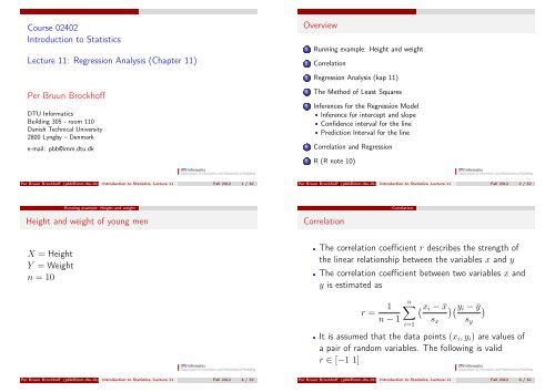
Course 02402<strong>Introduction</strong> <strong>to</strong> <strong>Statistics</strong><strong>Lecture</strong> <strong>11</strong>: <strong>Regression</strong> <strong>Analysis</strong> (<strong>Chapter</strong> <strong>11</strong>)Overview1 Running example: Height and weight2 Correlation3 <strong>Regression</strong> <strong>Analysis</strong> (kap <strong>11</strong>)Per Bruun BrockhoffDTU InformaticsBuilding 305 - room <strong>11</strong>0Danish Technical University2800 Lyngby – Denmarke-mail: pbb@imm.dtu.dk4 The Method of Least Squares5 Inferences for the <strong>Regression</strong> ModelInference for intercept and slopeConfidence interval for the linePrediction Interval for the line6 Correlation and <strong>Regression</strong>7 R (R note 10)Per Bruun Brockhoff (pbb@imm.dtu.dk) <strong>Introduction</strong> <strong>to</strong> <strong>Statistics</strong>, <strong>Lecture</strong> <strong>11</strong> Fall 2012 1 / 32Per Bruun Brockhoff (pbb@imm.dtu.dk) <strong>Introduction</strong> <strong>to</strong> <strong>Statistics</strong>, <strong>Lecture</strong> <strong>11</strong> Fall 2012 2 / 32Running example: Height and weightHeight and weight of young menCorrelationCorrelationX = HeightY = Weightn = 10The correlation coefficient r describes the strength ofthe linear relationship between the variables x and yThe correlation coefficient between two variables x andy is estimated asr = 1n − 1n∑ (x i − ¯x )(y i − ȳ)s yi=1It is assumed that the data points (x i , y i ) are values ofa pair of random variables. The following is validr ∈ [−1 1]s xPer Bruun Brockhoff (pbb@imm.dtu.dk) <strong>Introduction</strong> <strong>to</strong> <strong>Statistics</strong>, <strong>Lecture</strong> <strong>11</strong> Fall 2012 4 / 32Per Bruun Brockhoff (pbb@imm.dtu.dk) <strong>Introduction</strong> <strong>to</strong> <strong>Statistics</strong>, <strong>Lecture</strong> <strong>11</strong> Fall 2012 6 / 32
Correlations computationsCorrelation<strong>Regression</strong> <strong>Analysis</strong> (kap <strong>11</strong>)<strong>Regression</strong> <strong>Analysis</strong> (<strong>Chapter</strong> <strong>11</strong>)We assume that Y is a s<strong>to</strong>chastic variable. We areinterested in modelling Y ’s dependency on anexplana<strong>to</strong>ry variable xWe look at a linear relationship between Y and x, thatis a regression model on the formY = α + βx + εPer Bruun Brockhoff (pbb@imm.dtu.dk) <strong>Introduction</strong> <strong>to</strong> <strong>Statistics</strong>, <strong>Lecture</strong> <strong>11</strong> Fall 2012 7 / 32Per Bruun Brockhoff (pbb@imm.dtu.dk) <strong>Introduction</strong> <strong>to</strong> <strong>Statistics</strong>, <strong>Lecture</strong> <strong>11</strong> Fall 2012 9 / 32<strong>Regression</strong> <strong>Analysis</strong> (kap <strong>11</strong>)Simple Linear <strong>Regression</strong><strong>Regression</strong> <strong>Analysis</strong> (kap <strong>11</strong>)Simple Linear <strong>Regression</strong>Y = α + βx} {{ }model+ ε }{{}residual**Y dependent variable**x independent variableα intercept with Y-axisβ slope*** **ε residual (random error)Per Bruun Brockhoff (pbb@imm.dtu.dk) <strong>Introduction</strong> <strong>to</strong> <strong>Statistics</strong>, <strong>Lecture</strong> <strong>11</strong> Fall 2012 10 / 32Per Bruun Brockhoff (pbb@imm.dtu.dk) <strong>Introduction</strong> <strong>to</strong> <strong>Statistics</strong>, <strong>Lecture</strong> <strong>11</strong> Fall 2012 <strong>11</strong> / 32
The Method of Least SquaresThe Method of Least SquaresThe Method of Least SquaresThe Method of Least Squaresa and b are determined byb = S xyS xxa = ȳ − b · ¯xa and b are the values that give the regression line thatminimizes the squared distance between the points andthe linea is an estimate for α and b is an estimate for βPer Bruun Brockhoff (pbb@imm.dtu.dk) <strong>Introduction</strong> <strong>to</strong> <strong>Statistics</strong>, <strong>Lecture</strong> <strong>11</strong> Fall 2012 17 / 32In the example we getS xx =S yy =S xy =n∑(x i − ¯x) 2 = 143i=1n∑(y i − ȳ) 2 = 31533i=1n∑(x i − ¯x)(y i − ȳ) = 2<strong>11</strong>9i=1along with ¯x = 6.50 and ȳ = 100.67Per Bruun Brockhoff (pbb@imm.dtu.dk) <strong>Introduction</strong> <strong>to</strong> <strong>Statistics</strong>, <strong>Lecture</strong> <strong>11</strong> Fall 2012 18 / 32The Method of Least SquaresThe Method of Least SquaresInferences for the <strong>Regression</strong> ModelInferences for the <strong>Regression</strong> ModelEstimates for α and β:The model is:b = S xyS xx= 2<strong>11</strong>9143 = 14.82a = ȳ − b · ¯x = 100.67 − 14.82 · 6.50 = 4.34ŷ = 4.34 + 14.82 · xWe assume that the observed data (Y i , x i ) can bedescribed by the modelY i = α + βx i + ε iwhere it is assumed that ε i are independent normallydistributed s<strong>to</strong>chastic variables with mean 0 and constantvariance σ 2An estimate of σ 2 iss 2 e = S yy − (S xy ) 2 /S xxn − 2Per Bruun Brockhoff (pbb@imm.dtu.dk) <strong>Introduction</strong> <strong>to</strong> <strong>Statistics</strong>, <strong>Lecture</strong> <strong>11</strong> Fall 2012 19 / 32Per Bruun Brockhoff (pbb@imm.dtu.dk) <strong>Introduction</strong> <strong>to</strong> <strong>Statistics</strong>, <strong>Lecture</strong> <strong>11</strong> Fall 2012 21 / 32
Inferences for the <strong>Regression</strong> ModelInference for intercept and slopeInference for intercept and slopeInferences for the <strong>Regression</strong> ModelInferences for intercept and slopeInference for intercept and slopeWe want <strong>to</strong> test the hypotheses about the intercept withthe y-axisThe test statistic ist =H 0 :H 1 :α = aα ≠ a√(a − α) nS xxs e S xx + n(¯x) 2The critical value is found in the t-distribution, t α/2 (n − 2)We want <strong>to</strong> test a hypothesis about the slope βThe test statistic ist =H 0 :H 1 :β = bβ ≠ b(b − β) √Sxxs eThe critical value is found in the t-distribution, t α/2 (n − 2)Per Bruun Brockhoff (pbb@imm.dtu.dk) <strong>Introduction</strong> <strong>to</strong> <strong>Statistics</strong>, <strong>Lecture</strong> <strong>11</strong> Fall 2012 22 / 32Per Bruun Brockhoff (pbb@imm.dtu.dk) <strong>Introduction</strong> <strong>to</strong> <strong>Statistics</strong>, <strong>Lecture</strong> <strong>11</strong> Fall 2012 23 / 32Inferences for the <strong>Regression</strong> ModelConfidence Intervals for α and βInference for intercept and slopeInferences for the <strong>Regression</strong> ModelConfidence Interval for α + βx 0Confidence interval for the lineConfidence interval for αConfidence interval for βa ± t α/2 · s e√1n + (¯x)2S xxb ± t α/2 · s e1√SxxA confidence interval for α + βx 0 corresponds <strong>to</strong> aconfidence interval at the point x 0√1(a + bx 0 ) ± t α/2 · s en + (x 0 − ¯x) 2S xxPer Bruun Brockhoff (pbb@imm.dtu.dk) <strong>Introduction</strong> <strong>to</strong> <strong>Statistics</strong>, <strong>Lecture</strong> <strong>11</strong> Fall 2012 24 / 32Per Bruun Brockhoff (pbb@imm.dtu.dk) <strong>Introduction</strong> <strong>to</strong> <strong>Statistics</strong>, <strong>Lecture</strong> <strong>11</strong> Fall 2012 25 / 32
Inferences for the <strong>Regression</strong> ModelPrediction Interval for α + βx 0Prediction Interval for the lineCorrelation and <strong>Regression</strong>Correlation and <strong>Regression</strong>Correlation coefficient and slope:A prediction interval for α + βx 0 corresponds <strong>to</strong> aprediction interval for the model at the point x 0(a + bx 0 ) ± t α/2 · s e√1 + 1 n + (x 0 − ¯x) 2S xxThe prediction interval will be bigger than the confidenceinterval for fixed αPer Bruun Brockhoff (pbb@imm.dtu.dk) <strong>Introduction</strong> <strong>to</strong> <strong>Statistics</strong>, <strong>Lecture</strong> <strong>11</strong> Fall 2012 26 / 32r =√Sxx√Syyb,r 2 = S xxS yyb 2The correlation r describes the strength a of linearrelation.The correlation squared r 2 expresses the proportion ofthe y variability explained by the linear relation.S yy = Variation explained by line +Unexplained variation( )S yy = S2 xyS xx+ S yy − S2 xyS xxPer Bruun Brockhoff (pbb@imm.dtu.dk) <strong>Introduction</strong> <strong>to</strong> <strong>Statistics</strong>, <strong>Lecture</strong> <strong>11</strong> Fall 2012 28 / 32Correlation and <strong>Regression</strong>Inference for CorrelationR (R note 10)R (R note 10)Assumes that both y and x are s<strong>to</strong>chastic (NOT only y)r is an estimate for ρ - the true linear relationshipbetween y and x.Page 340-341 (7ed: 380-381): Formulae for hypothesistests and confidence intervals for the correlationcoefficient.ρ = 0 corresponds <strong>to</strong> β = 0r = 0 corresponds <strong>to</strong> b = 0Hypotheses test for ρ = 0 can be carried out by testingβ = 0> fit.evap summary(fit.evap)Call: lm(formula = evap ~ velocity)Residuals:Min 1Q Median 3Q Max-0.201 -0.1467 0.05261 0.1232 0.1747Coefficients:Value Std. Error t value Pr(>|t|)(Intercept) 0.0692 0.1010 0.6857 0.5123velocity 0.0038 0.0004 8.7460 0.0000Residual standard error: 0.1591 on 8 degrees of freedomMultiple R-Squared: 0.9053F-statistic: 76.49 on 1 and 8 degrees of freedom,the p-value is 2.286e-05Per Bruun Brockhoff (pbb@imm.dtu.dk) <strong>Introduction</strong> <strong>to</strong> <strong>Statistics</strong>, <strong>Lecture</strong> <strong>11</strong> Fall 2012 29 / 32Per Bruun Brockhoff (pbb@imm.dtu.dk) <strong>Introduction</strong> <strong>to</strong> <strong>Statistics</strong>, <strong>Lecture</strong> <strong>11</strong> Fall 2012 31 / 32
R (R note 10)Oversigt1 Running example: Height and weight2 Correlation3 <strong>Regression</strong> <strong>Analysis</strong> (kap <strong>11</strong>)4 The Method of Least Squares5 Inferences for the <strong>Regression</strong> ModelInference for intercept and slopeConfidence interval for the linePrediction Interval for the line6 Correlation and <strong>Regression</strong>7 R (R note 10)Per Bruun Brockhoff (pbb@imm.dtu.dk) <strong>Introduction</strong> <strong>to</strong> <strong>Statistics</strong>, <strong>Lecture</strong> <strong>11</strong> Fall 2012 32 / 32


