Russian Journal of Agricultural and Socio-Economic Sciences ...

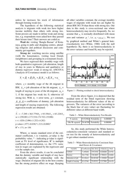
SULTANA NAYEEM, University of Dhakaunless he increases his stock of informationthrough forming weak ties.The hypothesis of the following statisticalanalysis is migrants with weak ties have higherincome mobility than others with strong ties.Some proxies are made to define weak and strongties, e.g. respondents were asked how they passedtheir leisure time? Their answers are coded as:Weak tie: visiting ‘Bangla Bazaar’ of Kotaraya,going to pubs and shopping centres, attendingreligious and political discussion and communityget togethers.Strong tie: watching movies using satellite(with the housemates), visiting local friends(neighbours) and gossiping in a restaurant (local).We have regressed their monthly wage withboth quantitative regressors: job alteration, lengthof stay in years in Malaysia and qualitative ordummy regressor: weak or strong tie. ANCOVA(Analysis of Covariance) model is as follows:Yi= β1 + β2D2i+ β3X2i+ β4X3i+ ui,where, Y = monthly wage of the ith migrant iniRM, X 2= job alteration of the ith migrant,iX 3=ilength of staying in years of the ith migrant, D 2=i1, if the migrant has weak tie; 0, otherwise (ifstrong tie). With ui= error term, β = constant,1β2, β3,β = coefficients of dummy, job alteration4and length of staying respectively. The followingregression results are obtained:∧Y i = −7 .295 + 363.779D2i+ 93.556X2i+ 83. 228X3ise = (250.001) (173.518) (74.742) (19.806)t = (-.029) (2.096) (1.252) (4.202)p-value= (.977) (0.038)* (.213) (0.000)*R 2 = .171, n= 150Where, se means standard error of the estimatedcoefficient, t is t-statistic, p-value is theprobability value, * - indicating p-value is significantat 5% level of significance, R 2 is multiplecoefficient of determination, i.e. the 17% variationin wages are explained by the regressors andn is the sample size.From the above results, it can be concludedthat the dummy variable and length of stay havestatistically significant relationship with thewage. Duration of migrant life in the host countryhas the strong positive effect on wage. Keepingall other variables constant, the average monthlywages of migrants with weak ties are higher byabout RM 363.78 than those with strong ties. Ourdata in this study is cross-sectional one whereheteroscedasticity may involve frequently. So, weassume that u is normally distributed with meani22zero and variance σ , i.e. u ~ii N(0,σi) . We testby graphical method and White’s general heteroscedasticitytest (White, 1980) with the nullhypothesis: H 0 : there is no heteroscedasticity inthe error variance and found H 0 may be rejected.4000300020001000-1000-2000020 40 60 80 100 120 140Residual Actual FittedFigure 1 – Plotting residual to check heteroscedasticyFrom the above figure, it is depicted that theresidual term of the fitted regression showingheteroscedasticity for different values of the regressors.The variances of the error (according tothe black line of zero value) are fluctuating fordifferent values at different band width.Table 2 – White Heteroskedasticity Test ResultsF-statistic 9.932964 Probability 0.000000Obs*R-squared 38.46709 Probability 0.0000008000600040002000So, this study performed the White heteroscedasticity-consistentvariances and standard errortest for the remedy of heteroscedasticity andto get robust standard errors.Table 3 – White Heteroskedasticity-Consistent StandardErrors & CovarianceVariable Coefficient Std. Error t-Statistic Prob.CONST -7.295058 279.9356 -0.026060 0.9792Dummy 363.7786 130.4603 2.788424 0.0060Alteration of job 93.55614 82.85140 1.129204 0.2607Length of staying 83.22766 33.05351 2.517968 0.0129011