A Mini-course on EllipticâHyperbolic Equations - ICMS
A Mini-course on EllipticâHyperbolic Equations - ICMS
A Mini-course on EllipticâHyperbolic Equations - ICMS

Create successful ePaper yourself
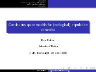
Turn your PDF publications into a flip-book with our unique Google optimized e-Paper software.
A <str<strong>on</strong>g>Mini</str<strong>on</strong>g>-<str<strong>on</strong>g>course</str<strong>on</strong>g> <strong>on</strong> Elliptic–Hyperbolic Equati<strong>on</strong>sThomas H. Otway<strong>ICMS</strong> Workshop in Differential Geometry & C<strong>on</strong>tinuumMechanics17–21 June 2013
Goal of the <str<strong>on</strong>g>course</str<strong>on</strong>g>: To illustrate the variety of c<strong>on</strong>texts in whichelliptic–hyperbolic equati<strong>on</strong>s arise, the variety of methods used toattack them, and the variety of ideas from analysis, geometry, andphysics that c<strong>on</strong>tribute to understanding them.
Part I. Orientati<strong>on</strong>◮ Why study this subject?◮ The analytic approach versus geometric approach◮ The linear theory versus the n<strong>on</strong>linear theory◮ The hodograph transformati<strong>on</strong>◮ The partial hodograph transformati<strong>on</strong>Part II. Elliptic–hyperbolic boundary value problems◮ Open versus closed boundary c<strong>on</strong>diti<strong>on</strong>s◮ What is the natural boundary geometry?◮ Weak soluti<strong>on</strong>s◮ “Almost-correct” boundary c<strong>on</strong>diti<strong>on</strong>s
Naive discussi<strong>on</strong> of equati<strong>on</strong> type:Physically, what do soluti<strong>on</strong>s of partial differential equati<strong>on</strong>s do?In general, they◮ propagate as waves◮ diffuse as heat◮ do nothing at all (e.g., “oscillate”)This leads to classificati<strong>on</strong> of the corresp<strong>on</strong>ding equati<strong>on</strong>s as,respectively◮ hyperbolic◮ parabolic◮ elliptic
But, for example:◮ Separating variables in Laplace’s equati<strong>on</strong> in toroidalcoordinates produces a partial differential equati<strong>on</strong> which iselliptic inside the unit circle and hyperbolic <strong>on</strong> theR 2 -complement of the unit circle;[B. Riemann, Partielle Differentialgleichungen, 1861; also C.Neumann, 1864; W. M Hicks, 1881; E. Heine, 1881; A. B.Basset, 1893]◮ the equati<strong>on</strong>s for a steady, irrotati<strong>on</strong>al, isentropic,compressible flow are elliptic for velocities below the speed ofsound in the medium, and hyperbolic at velocities above thespeed of sound;[H. Bateman, Proc. R. Soc. L<strong>on</strong>d<strong>on</strong> Ser. A 125 (1929)]
◮ The c<strong>on</strong>tinuity equati<strong>on</strong>s for shallow water are elliptic whenthe flow speed is below a certain value (the Froude number)and hyperbolic when the speed exceeds that value;[<strong>on</strong>e space dimensi<strong>on</strong>: D. Riabouchinsky, C. R. Acad, Sci.Paris 195 (1932); two space dimensi<strong>on</strong>s: J. J. Stoker,Commun. Pure Appl. Math. 1 (1948)]◮ the governing equati<strong>on</strong>s in a c<strong>on</strong>tinuum model for two-lanetraffic flow in opposing directi<strong>on</strong>s change from hyperbolic toelliptic type over a regi<strong>on</strong> of phase space, provided aparameter is introduced which represents a degree ofdependence between the flow density in each lane and theflow density in the opposing lane – the area of the ellipticregi<strong>on</strong> depends <strong>on</strong> the strength of the interacti<strong>on</strong> parameter;[J. H. Bick and G. F. Newell, Quart. Appl. Math. 18, (1960)]
◮ the governing equati<strong>on</strong>s for ideal magnetohydrodynamic flowin a nozzle change between elliptic and hyperbolic type threetimes: at the sound speed c, the Alfvén speed a, and thespeed: ca/ √ c 2 + a 2 ;[C. K. Chu, Phys. Fluids 5 (1962)]◮ the complex eik<strong>on</strong>al equati<strong>on</strong> is of hyperbolic type in theinterior of a circular caustic and of elliptic type <strong>on</strong> the exteriorof the caustic;[Yu. A. Kravtsov, Radiofizika 7 (1964); also D. Ludwig,Commun. Pure Appl. Math. 19 (1966); R. Magnanini and G.Talenti, C<strong>on</strong>temporary Math. 283, (1999)]
◮ the equati<strong>on</strong>s for a magnetic field applied to azero-temperature plasma are elliptic at certain frequencies ofthe applied field and hyperbolic at other frequencies;[for electrostatic waves: A. D. Piliya and V. I. Fedorov, Sov.Phys. JETP 33 (1971); for fully electromagnetic waves: H.Weitzner, Commun. Pure Appl. Math. 38 (1985)]◮ the governing equati<strong>on</strong>s of a simple model for l<strong>on</strong>gitudinal (orfor pure shearing) moti<strong>on</strong>s are strictly hyperbolic undertensi<strong>on</strong> and of mixed equati<strong>on</strong> type under compressi<strong>on</strong>;[J. L. Ericksen, J. Elasticity 5 (1975)]
◮ the Laplace–Beltrami equati<strong>on</strong> <strong>on</strong> the extended projective discP 2 is elliptic inside the Beltrami disc but hyperbolic outside ofit;[L-K. Hua, Proc. 1980 Beijing Symp. Diff. Geometry Diff.Equati<strong>on</strong>s 1 (1982); some hints in the work of G. G. Stokes,1854]◮ by a series of approximati<strong>on</strong>s, the partiti<strong>on</strong> functi<strong>on</strong> forquantum electrodynamics can be reduced to a relativisticmodel in which the quarks are coupled to a pair of classicalgauge fields. Additi<strong>on</strong>al choices reduce the analysis to aproblem in n<strong>on</strong>linear electrostatics which change from ellipticto hyperbolic type depending <strong>on</strong> the value of a (highlyn<strong>on</strong>linear) functi<strong>on</strong> of the flux, its gradient, and the radialcoordinate;[S. L. Adler and T. Piran, Phys. Lett. 113B (1982)]
◮ according to the Hartle–Hawking model, the Laplace–Beltramiequati<strong>on</strong> <strong>on</strong> a matter-free regi<strong>on</strong> of space-time would havebeen of elliptic type in the early universe and would havechanged to an equati<strong>on</strong> of hyperbolic type across ahypersurface which is space-like when viewed from the present;[J. B. Hartle and S. W. Hawking, Phys. Rev. D 28 (1983)]◮ some models for multiphase flow change from hyperbolic toelliptic type;[Review: B. L. Keyfitz, Change of type in simple models oftwo-phase flow, 1992.]
◮ In certain models for plasma flow in a tokamak, the governingequati<strong>on</strong> changes its type twice: from elliptic to hyperbolicand back again, with increasing flow velocity. However, thewidth of the hyperbolic regi<strong>on</strong> (whether negligible or not) inat least some of the models is a matter of c<strong>on</strong>troversy.[A. Lifschitz and J. P. Goedbloed, J. Plasma Phys. (1997);also E. Hamieri, L. Guazzotto, unpublished, 2012]◮ the wave equati<strong>on</strong> in Minkowski space-time, in a referenceframe rotating with c<strong>on</strong>stant angular velocity with respect toanother reference frame, is elliptic for certain values of theradial coordinate and hyperbolic for other values;[J. M. Stewart, Classical Quant. Grav. 18 (2001)]
◮ the helically reduced wave equati<strong>on</strong> <strong>on</strong> a torus (a qualitativelinear model for the reducti<strong>on</strong> of the Einstein equati<strong>on</strong>s by ahelical Killing vector field) is elliptic for certain values of theradial coordinate and hyperbolic for other values;[C. G. Torre, J. Math. Phys. 44 (2003); C. Klein, Phys. Rev.D 70 (2004)]◮ An equati<strong>on</strong> arising in the design of automobile windshieldschanges from elliptic to hyperbolic type as a certain shapeparameter of the windshield is varied;[N. Bîlă, SIAM J. Appl. Math. 65, (2004)]
◮ The relevant equati<strong>on</strong> for the existence of an isometricembedding of Riemannian surfaces in higher-dimensi<strong>on</strong>alEuclidean space is either hyperbolic or elliptic depending <strong>on</strong>the sign of the curvature (the same is true for the equati<strong>on</strong>governing the existence of a surface having prescribedGaussian curvature);[Review: Q.Han and J.-X.H<strong>on</strong>g, Isometric Embedding ofRiemannian Manifolds in Euclidean Spaces (2006) – theproblem goes back <strong>on</strong>e way or another to Schlaefli in 1873]etc., etc., etc.... It is quite comm<strong>on</strong> for soluti<strong>on</strong>s to change theirnature (oscillatory to propagating) across a smooth curve in theirdomain. The associated partial differential equati<strong>on</strong>s are calledelliptic–hyperbolic.
Two approaches to elliptic–hyperbolic equati<strong>on</strong>s◮ basically analytic (tends to arise in c<strong>on</strong>tinuum mechanics)◮ basically geometric (tends to arise in relativistic mechanics)Analytic approach − applies to a class of equati<strong>on</strong>s <strong>on</strong> a fixed,generic domain.C<strong>on</strong>sider a fixed domain Ω ⊂ R n (in this <str<strong>on</strong>g>course</str<strong>on</strong>g> we almost alwaystake n = 2) and the class of differential operators having thefollowing higher-order terms:Lu = αu xx + 2βu xy + γu yyα, β, and γ are given functi<strong>on</strong>s of the coordinates (x, y) ∈ Ω; u isan unknown functi<strong>on</strong> of x and y.If ∆ ≡ αγ − β 2 < 0, then the characteristic linesαdy 2 − 2βdxdy + γdx 2 = 0are real-valued and soluti<strong>on</strong>s propagate as waves.
Adopting the “differential polynomial” approach to classificati<strong>on</strong>,we replace the sec<strong>on</strong>d-order derivatives by quadratic algebraicterms and obtain a classificati<strong>on</strong> for differential operatorsanalogous to the classificati<strong>on</strong> of quadratic surfaces:∆ = αγ − β 2 ⎧⎨⎩corresp<strong>on</strong>ding to “elliptic,” “hyperbolic,” “parabolic” equati<strong>on</strong>s,respectively.If ∆ changes sign <strong>on</strong> a smooth “s<strong>on</strong>ic” (“parabolic”) curve <strong>on</strong> thedomain, then the equati<strong>on</strong> associated with L is said to be of mixedelliptic–hyperbolic type.>
A linear example [Lavrent’ev & Bitsadze, Dokl. Akad. Nauk 20(1950)]:Lu = sgn[y]u xx + u yy = 0,for which the s<strong>on</strong>ic curve is the x-axis.Laplace’s equati<strong>on</strong> <strong>on</strong> the upper half-planeWave equati<strong>on</strong> <strong>on</strong> the lower half plane.A quasilinear example [S-X. Chen, Acta Math. Sci. 31B (2011)]:sgn[u]u xx + u yy = 0,a model for the reflecti<strong>on</strong> of certain shock waves in compressiblegas dynamics.In the n<strong>on</strong>linear case the s<strong>on</strong>ic curve cannot be identified withoutsolving the equati<strong>on</strong>.
Example of a first-order elliptic–hyperbolic systemA scalar equati<strong>on</strong> arising in, e.g., n<strong>on</strong>linear elasticitywhere x ∈ R and t ∈ R + .u tt = σ (u x ) x, (1)Assumpti<strong>on</strong>s <strong>on</strong> the stress functi<strong>on</strong> σ that lead to a change inequati<strong>on</strong> type: ∃ α, β, γ, and δ such that, e.g.,
This is equivalent to the systemw t = v x , v t = σ(w) x .We can impose initial values w (x, 0) = w 0 (x) and v (x, 0) = v 0 (x).Equating mixed partial derivatives of v yieldsw tt = σ(w) xx ,and making the substituti<strong>on</strong>s w = u x and v = u t , yieldsu tt = σ (u x ) x,which is eq. (1) of the preceding frame.[Pego and Serre, SIAM J. Numer. Anal. 25 (1988); Bo<strong>on</strong>kasameand Milewski, Studies in Appl. Math. 128 (2011); Bialy andMir<strong>on</strong>ov, arXiv e-print, December 2012]
We obtain from the first-order system the matrix equati<strong>on</strong>( ) ( ) ( )w 0 1 w=v σ ′ .(w) 0 vtThis is of <str<strong>on</strong>g>course</str<strong>on</strong>g> a matrix equati<strong>on</strong> of the form X t = AX x . Nowadopting the “eigenvalue approach” to classificati<strong>on</strong>, we computethe eigenvalues of the matrix −A by solving the scalar equati<strong>on</strong>|A + λI | =∣Because the eigenvaluesλ 1σ ′ (w) λλ = ± √ σ ′ (w)∣ = λ2 − σ ′ (w) = 0.are real-valued and n<strong>on</strong>degenerate when σ ′ is positive, in that casethe characteristics are real and we take this to be the regi<strong>on</strong> ofhyperbolicity for the system.Remark: classical soluti<strong>on</strong>s of this equati<strong>on</strong> tend to havefinite-time singularities even in the strictly hyperbolic regime, so weusually look for weak soluti<strong>on</strong>s.x
Making the choice σ(t) = t 2 in the preceding discussi<strong>on</strong> leads toequati<strong>on</strong>s of Boussinesq type, which arise in hydrodynamics. Weview these as first-order systems u t + B(u)u x = 0, takingu = (h, w) T , whereB(u) =(−hw1−w 21−h222−hwThe sub-domain of hyperbolic soluti<strong>on</strong>s, that is, the domain ofwave moti<strong>on</strong>, coincides with that regi<strong>on</strong> of the domain <strong>on</strong> whichthe eigenvalues of B, that is, the numbers)√(1 − hλ ± B = −hw ± 2 ) (1 − w 2 ),2are real and the associated eigenvectors span R 2 . That corresp<strong>on</strong>dsto the regi<strong>on</strong> in which |h| and |w| are both less than 1. This is asquare, not in the xt-plane but in the “phase space” of thehw-plane – a square which cannot be determined without solvingthe system..
Geometric approach: replace the class of differential operators L<strong>on</strong> a fixed, generic domain with a fixed, generic differentialoperator L <strong>on</strong> a class of domains (M, g) .Laplace–Beltrami operator:L g u = 1 √|g|∂∂x i (g ij√ |g| ∂u∂x j ),<strong>on</strong> a class of manifolds for which the matrix g ij represents the localmetric tensor having determinant g.
Geometric interpretati<strong>on</strong> of the (linear) Lavrent’ev–Bitsadzeequati<strong>on</strong>Lu = sgn[y]u xx + u yy = 0,g is Euclidean above the x-axis:with signature (+, +)ds 2 = dx 2 + dy 2 ,and Minkowskian below the x-axis:with signature (+, −) .In general:ds 2 = dx 2 − dy 2 ,◮ elliptic operators ⇐⇒ Riemannian (“Euclidean”) metrics◮ hyperbolic operators ⇐⇒ semi-Riemannian (typically,Lorentzian) metrics.
Four features of the geometric approach:◮ The type of a linear sec<strong>on</strong>d-order equati<strong>on</strong> is not a functi<strong>on</strong> ofthe associated linear operator at all, as that operator is alwaysthe Laplace–Beltrami operator. Instead, the type of theequati<strong>on</strong> is a feature of the metric tensor <strong>on</strong> the underlyingpseudo-Riemannian manifold.◮ Any change in signature which results in a change in sign ofthe metric determinant g will change the Laplace–Beltramioperator <strong>on</strong> the metric from elliptic to hyperbolic type.◮ In order to decide which boundary value problems are naturalfor a sec<strong>on</strong>d-order linear elliptic–hyperbolic equati<strong>on</strong>, <strong>on</strong>eshould study the geometry of the underlying metric.◮ Any curve <strong>on</strong> which the change of type occurs will necessarilyrepresent a singularity of the metric tensor, as g will vanishal<strong>on</strong>g that curve. However, n<strong>on</strong>e of the terms in the equati<strong>on</strong>itself need blow up <strong>on</strong> this curve. (An example is the waveequati<strong>on</strong> <strong>on</strong> extended P 2 .)
The linear theoryWhy bother with the linear theory of elliptic–hyperbolic equati<strong>on</strong>s?Two arguments against emphasizing <strong>on</strong> the linear theory:“The linear theory of elliptic equati<strong>on</strong>s extends in a qualitativesense to much of the n<strong>on</strong>linear theory, but n<strong>on</strong>linear hyperbolicequati<strong>on</strong>s are much more singular than in the linear case, so thelinear elliptic–hyperbolic theory is not much of a guide to n<strong>on</strong>linearequati<strong>on</strong>s, which are the <strong>on</strong>es of real interest.”“In the important applicati<strong>on</strong>s, linear elliptic–hyperbolic equati<strong>on</strong>sare <strong>on</strong>ly associated with small initial data.”Five reas<strong>on</strong>s for developing a sound linear theory:
1. Elliptic–hyperbolic c<strong>on</strong>tinuity equati<strong>on</strong>s tend to arise in specialforms which allow linearizati<strong>on</strong> by the hodograph method. Theseequati<strong>on</strong>s are more ubiquitous than people think (see below), andthe hodograph method is more useful than people think (see, forexample, the work of Yuxi Zheng)2. In, e.g., plasma c<strong>on</strong>texts, linear elliptic–hyperbolic models arisepartly from certain physical hypotheses, for example:◮ magnetically dominated low-beta fields (“force-free models”)which arise in models of the solar cor<strong>on</strong>a, ball lightning, andintergalactic jets;◮ fields in which small-amplitude electromagnetic wavespropagate with a velocity much greater than the thermaloscillati<strong>on</strong>s of the particles (“cold plasma models”), whicharise in certain models of tokamak plasmas;◮ equilibrium models, in which a steady plasma is surrounded bya vacuum [R. Temam, Arch. Rat. Mech. Anal. 60, (1975)].
3. The presence of an elliptic regi<strong>on</strong> can exert a regularizing effect<strong>on</strong> the hyperbolic regi<strong>on</strong> (e.g., elliptic–hyperbolic models ofcaustics in which boundary data can be prescribed in the ellipticregi<strong>on</strong>, which surrounds the hyperbolic regi<strong>on</strong>), making theanalogy to n<strong>on</strong>linear hyperbolic pde less apt.4. Few experts in n<strong>on</strong>linear waves would prefer not to have a goodlinear theory of hyperbolic equati<strong>on</strong>s.5. An understanding of the linear theory is necessary in order tosolve n<strong>on</strong>linear partial differential equati<strong>on</strong>s locally byimplicit-functi<strong>on</strong> methods:
Denote by Ω a domain of R n and c<strong>on</strong>sider the solvability of an<strong>on</strong>linear partial differential equati<strong>on</strong> F (u) = f , where f lies in thefuncti<strong>on</strong> space H k (Ω). If D p is a fixed open set of H p , then wewant to solve this equati<strong>on</strong> for u ∈ D p . It is generally possible tofind an approximate soluti<strong>on</strong> u 0 such that F (u 0 ) is “close” to f insome useful sense. The goal is to use some versi<strong>on</strong> of the ImplicitFuncti<strong>on</strong> Theorem to perturb u 0 locally into a local soluti<strong>on</strong> to theequati<strong>on</strong> F (u) = f . The solvability of the n<strong>on</strong>linear equati<strong>on</strong>depends critically <strong>on</strong> the invertibility at u 0 of the linear operatorF ′ (u) v = d dt |t=0F (u + tv) .(There are technical problems c<strong>on</strong>nected with this method.) Twoimportant classes of n<strong>on</strong>linear elliptic–hyperbolic problems ingeometry have been attacked in this way.
The isometric embedding problem: When can a 2-dimensi<strong>on</strong>alRiemannian manifold be “seen” via a local realizati<strong>on</strong> in R 3 ? Thisproblem is associated with the existence of a local soluti<strong>on</strong> to thefully n<strong>on</strong>linear Darboux equati<strong>on</strong>. But that equati<strong>on</strong> has beensuccessfully approached via Nash–Moser methods involving thelinearizati<strong>on</strong>(aKu x ) x+ bu yy + cKu x + du y ,where a, b > 0 and K is the Gaussian curvature of the surface.[Han, Commun. Pure Appl. Math. 58 (2005); Han and Khuri,Commun. Anal. Geom. 18 (2010)]
Given a functi<strong>on</strong> K (x, y) defined in a neighborhood of the origin,does there exist a graph z (x, y) having Gaussian curvature K?Because every surface may be expressed locally as a graph, this isthe problem of locally prescribing the curvature of a surface. As inthe preceding geometric problem, this problem can be reduced tothe local solvability of a M<strong>on</strong>ge–Ampère equati<strong>on</strong>, and in this caseas well implicit-functi<strong>on</strong> methods lead <strong>on</strong>e to c<strong>on</strong>sider the linearequati<strong>on</strong>u yy + ( x 2 − y 2) u xx = f .[Q. Han and M. Khuri, Calc. Var. Partial Diff. Eqs. (2012)]
Local can<strong>on</strong>ical forms for linear equati<strong>on</strong>sThe two can<strong>on</strong>ical forms for linear, sec<strong>on</strong>d-order elliptic–hyperbolicequati<strong>on</strong>s were discovered by Francesco Tricomi (left) and MariaCinquini-Cibrario (right).
For most of the past century, the study of linear elliptic–hyperbolicequati<strong>on</strong>s was generally identified with the study of the Tricomiequati<strong>on</strong>yu xx + u yy = 0.Typical domain: Ω ⊂⊂ R 2 bounded by a smooth Jordan curve γin the upper half plane and the characteristic linesΓ 1 : x − 2 3 (−y)3/2 = −1, x < 0,in the lower half-plane.Γ 2 : x + 2 3 (−y)3/2 = 1, x > 0,
Tricomi [Rend. Accad. Naz. Lincei Ser. 5 14 (1923)]:◮ A unique soluti<strong>on</strong> exists <strong>on</strong> Ω provided the values of u (x, y)are smoothly prescribed <strong>on</strong> the elliptic arc γ and thecharacteristic line Γ 2 (True).◮ Any sufficiently smooth equati<strong>on</strong> having the formα (x, y) u xx + 2β (x, y) u xy +γ (x, y) u yy + lower order terms = 0,for which the discriminant β 2 − αγ changes sign al<strong>on</strong>g asmooth curve, is locally equivalent to the equati<strong>on</strong>yu xx + u yy + lower order terms = 0 (False).
Tricomi’s assistant Cinquini-Cibrario realized that there wereelliptic–hyperbolic equati<strong>on</strong>s which are not locally equivalent toTricomi’s equati<strong>on</strong>. Example:xu xx + u yy = 0.(Old “NYU” name for this equati<strong>on</strong>: anti-Tricomi.)Boundary value problems have soluti<strong>on</strong>s <strong>on</strong> a domain which lookslike a Tricomi domain rotated clockwise by 90 ◦ . Red and bluecurves: Characteristics y = ∓ √ −x ± 4. Cinquini-Cibrario showedthat there exist classical soluti<strong>on</strong>s with data prescribed <strong>on</strong> theelliptic boundary.
Cinquini-Cibrario’s local can<strong>on</strong>ical forms [Rend. R. Inst. Lomb.65 (1932)]:L T ≡ y 2m+1 u xx + u yy + lower-order termsorL K ≡ u xx + y 2m+1 u yy + lower-order terms.(Here m is a n<strong>on</strong>-negative integer.)A differential equati<strong>on</strong> for which the differential operator L can betransformed locally into an operator of the form L T is said to be ofTricomi type.A differential equati<strong>on</strong> for which the differential operator L can betransformed locally into an operator of the form L K is said to be ofKeldysh type.
M.V. Keldysh had nothing to do with the discovery of either of thecan<strong>on</strong>ical forms. Twenty years later he studied the degenerati<strong>on</strong> ofellipticity in the class of equati<strong>on</strong>s introduced and studied byCinquini-Cibrario.[M. V. Keldysh, On certain classes of elliptic equati<strong>on</strong>s withsingularity <strong>on</strong> the boundary of the domain, Dokl. Akad. NaukSSSR 77 (1951)]
Alternative definiti<strong>on</strong> of the can<strong>on</strong>ical forms:We can always write a sec<strong>on</strong>d-order linear equati<strong>on</strong> with smoothcoefficients defined in an open set of R 2 in the local formLu = K (x, y) u xx + u yy + lower-order terms.One can, by a further n<strong>on</strong>singular transformati<strong>on</strong>, arrive at acoordinate system in which the type-change functi<strong>on</strong> K (x, y) haseither of two forms:1. K(y), with K(0) = 0 and yK(y) > 0 for y ≠ 0, or2. K(x), with K(0) = 0 and xK(x) > 0 for x ≠ 0.The former characterizes equati<strong>on</strong>s of Tricomi type and the latter,equati<strong>on</strong>s of Keldysh type.Still more generally, <strong>on</strong>e notices that the distincti<strong>on</strong> is <strong>on</strong>lymeaningful in a neighborhood of the s<strong>on</strong>ic curve.
Equati<strong>on</strong>s of Keldysh type can be characterized by thedegenerati<strong>on</strong> of their characteristic lines, which intersect s<strong>on</strong>iccurve tangentially (leading to weaker regularity):
Example of the weaker regularity of equati<strong>on</strong>s of Keldyshtype:Fundamental soluti<strong>on</strong>s are the main ingredient for solving theDirichlet problem by the Green’s functi<strong>on</strong> method.A fundamental soluti<strong>on</strong> exists for the Tricomi equati<strong>on</strong>[Barros-Neto & Gelfand, Duke Math. J. 98(1999)].A fundamental soluti<strong>on</strong> exists for the Keldysh equati<strong>on</strong> <strong>on</strong>ly as thefinite part of a divergent improper integral [S-X. Chen, Sci. inChina, Ser. A: Math. 52 (2009)].
Why do equati<strong>on</strong>s of Keldysh type have weaker regularity?C<strong>on</strong>sider a differential operator of order m > 0 <strong>on</strong> an open setΩ ⊂ R n ,Pu(x) = ∑ ( ) ∂ αc α (x) u(x),∂x|α|≤mξ α = ξ α 11 · · · ξαn n , having C ∞ real (for simplicity) coefficients. Theprincipal symbol of P is the functi<strong>on</strong>σ P (x, ξ) = ∑c α (x)ξ α .|α|=mIf P is of real principal type then, roughly speaking, all itssignificant properties are determined by its principal symbol.
In general, the operator P is of real principal type if at every pointx ∈ Ω its real characteristic c<strong>on</strong>eC (P, x) = {ξ ∈ R n | ξ ≠ 0, σ P (x, ξ) = 0}has no singular points. (If P is elliptic, then C is empty.)There are many equivalent c<strong>on</strong>diti<strong>on</strong>s for an operator to be of realprincipal type. In the c<strong>on</strong>crete case of an operator having the formLu = K (x, y) u xx + u yy + lower-order ,the operator L is of real principal type if whenever K (x, y) = 0, wealso have K y (x, y) ≠ 0.
Let ξ = K (x, y) and η = λ (x, y) . This produces an operator ofthe formLu ≡ Ku ξξ + γu ηηwhere λ has been chosen so that the following identities aresatisfied:KK x λ x + K y λ y = 0; (2)Kλ 2 x + λ 2 y = γ. (3)If K and K y never vanish simultaneously at the s<strong>on</strong>ic transiti<strong>on</strong>K = ξ = 0, then λ y is forced by (2) to vanish whenever Kvanishes; that is, λ y vanishes at the s<strong>on</strong>ic transiti<strong>on</strong>. But in thatcase, c<strong>on</strong>diti<strong>on</strong> (3) forces γ to also vanish at the s<strong>on</strong>ic transiti<strong>on</strong>.
Writing the characteristic equati<strong>on</strong> for Lu = 0, we haveKdη 2 + γdξ 2 = 0. (4)If K and K y can vanish simultaneously, then it is possible to haveγ ≠ 0 <strong>on</strong> the s<strong>on</strong>ic curve, in which case eq. (4) assumes the formγdξ 2 = 0, γ ≠ 0. So in the case K = 0 = K y the characteristiclines satisfy ξ = dξ = 0. That is, they degenerate <strong>on</strong> the s<strong>on</strong>iccurve, and the case K = 0 = K y corresp<strong>on</strong>ds to equati<strong>on</strong>s ofKeldysh type.A tedious algebraic calculati<strong>on</strong> will show directly that if K and K ydo not vanish simultaneously, then the operator L is of Tricomitype.That is to say, the Tricomi operator (K (x, y) = y) is of realprincipal type but the Keldysh operator (K (x, y) = x) is not, anda lower-order perturbati<strong>on</strong> of a well-behaved operator of Keldyshtype can be badly behaved.
Moreover the Implicit Functi<strong>on</strong> Theorem requires that when thelinear operator P is inverted, all the p derivatives lost in theoriginal linearizati<strong>on</strong> map are regained. That c<strong>on</strong>diti<strong>on</strong> is <strong>on</strong>lystrictly satisfied by so-called hypoelliptic operators. However, if Pis of real principal type, then an inverse exists that loses <strong>on</strong>ly <strong>on</strong>ederivative. That case is amenable to treatment by the Nash–Moseriterati<strong>on</strong>. So the “right” class of operators to c<strong>on</strong>sider when usingimplicit-functi<strong>on</strong> methods – not as restrictive as hypoellipticity, butrestrictive enough to satisfy the requirements of the Nash–Moseriterati<strong>on</strong> – is the class of operators of real principal type. That is,Nash–Moser arguments are well-adapted to linearizati<strong>on</strong>s which areoperators of Tricomi type, because they are of real principal type,but are not well-adapted to operators of Keldysh type.
The hodograph linearizati<strong>on</strong>Most of the analytic techniques for elliptic–hyperbolic equati<strong>on</strong>srequire linearity. Most of the elliptic–hyperbolic models in physicsare n<strong>on</strong>linear. But many of these models are in the very specialform required for linearizati<strong>on</strong> by the hodograph method.In its full generality, the hodograph transformati<strong>on</strong> is ann-dimensi<strong>on</strong>al method in which a functi<strong>on</strong> u(x), x ∈ R n , havingn<strong>on</strong>zero Hessian, is transformed locally by a mapping of the regi<strong>on</strong>into a new regi<strong>on</strong> given by the coordinate transformati<strong>on</strong>x → y = ∇u. The derivatives of u can then be expressed in termsof the derivatives of y via the Legendre transformati<strong>on</strong> u → v,wherev = x i y i − u = x i u x i − u.(Here and below, repeated indices are summed from 1 to n.) Thuspartial differential equati<strong>on</strong>s for u become equati<strong>on</strong>s for v.
If a system of equati<strong>on</strong>s has the form[ ] ( ) [ ] (a11 a 12 p b11 b+12 pa 22 qb 22 qa 21xb 21)y( 0=0), (5)where the entries of the coefficient matrices depend <strong>on</strong>ly <strong>on</strong> p andq, then the coordinate transformati<strong>on</strong> (x, y) → (p, q) takes eq. (5)into a linear equati<strong>on</strong> having the form[ ] ( ) [ ] ( ) ( )b12 −a 12 x −b11 a+11 x 0= .−a 22 ya 21 y 0b 22p−b 21This transformati<strong>on</strong> is called a hodograph map. It fails at anypoint for which its Jacobian J = p x q y − p y q x vanishes.q
This map is easy to understand as an inversi<strong>on</strong> of the differentialformsdp = p x dx + p y dyanddq = q x dx + q y dy.Written in matrix form, this is the system( ) ( ) ( dp px p=y dxdq q x q y dy),which has the inverse( ) dx= 1 dy Jprovided J is n<strong>on</strong>vanishing.−q x p x dq(qy −p y) ( dp)
The coordinate systems (p, q) and (x, y) are related by theLengendre transformati<strong>on</strong>V (p, q) = xp + yq − v(x, y), (6)where in this caseand(x, y) =(p, q) =( ∂V∂p , ∂V )∂q( ∂v∂x , ∂v ).∂y
Example of the use of the hodograph method: [Magnanini &Talenti, in: Ill-posed and Inverse Problems, VSP, (2002)]( )( )|∇θ| 4 − θy2 θ xx + 2θ x θ y θ xy + |∇θ| 4 − θx2 θ yy = 0. (7)This quasilinear elliptic–hyperbolic equati<strong>on</strong> arises in the c<strong>on</strong>text ofc<strong>on</strong>structing uniform asymptotic expansi<strong>on</strong>s of the Helmholtzequati<strong>on</strong> near a smooth, c<strong>on</strong>vex caustic.We can write this equati<strong>on</strong> as a homogeneous first-order system inp (x, y) and q (x, y) , with quasilinear term depending <strong>on</strong>ly <strong>on</strong> pand q.
Making the substituti<strong>on</strong>s p = θ x , q = θ y in the original quasilinearsystem (7), we apply the hodograph transformati<strong>on</strong> and eventuallyobtain the (now linear) scalar equati<strong>on</strong>[ (p 2 + q 2) 2− p2 ] V pp− 2pqV pq +[ (p 2 + q 2) 2− q2 ] V qq = 0, (8)provided there is a c<strong>on</strong>tinuously differentiable scalar functi<strong>on</strong>V (x, y) for which V p = x and V q = y.
Three limitati<strong>on</strong>s of the hodograph linearizati<strong>on</strong>◮ It requires that the equati<strong>on</strong> be of a very special form and isnot robust to small changes in that form.◮ The hodograph transformati<strong>on</strong> may be singular. (Butgenerally, any singular set <strong>on</strong> the elliptic regi<strong>on</strong> of theequati<strong>on</strong>s must c<strong>on</strong>sist of isolated points.)◮ Whereas the hodograph mapping replaces a quasilinearequati<strong>on</strong> by a linear <strong>on</strong>e, it tends to replace linear boundaryc<strong>on</strong>diti<strong>on</strong>s by n<strong>on</strong>linear <strong>on</strong>es. In general this restricts theboundary c<strong>on</strong>diti<strong>on</strong>s that can be applied in this method torelatively simple examples.Example: The vanishing of a soluti<strong>on</strong> to the Magnanini–Talentiequati<strong>on</strong> (8) <strong>on</strong> a circle in the hodograph plane pulls back, under ahodograph transformati<strong>on</strong>, to a c<strong>on</strong>stant value of the soluti<strong>on</strong> <strong>on</strong>the corresp<strong>on</strong>ding circle in the physical plane.
The partial hodograph transformati<strong>on</strong>This is a(nother) very old method that has attracted new interestrecently. Instead of switching all the dependent variables in theequati<strong>on</strong> with all the independent variables as in the classicalhodograph method, In this variant we switch just <strong>on</strong>e. (In theory,switching any number of dependent variables that is fewer than allof them will result in a partial hodograph transformati<strong>on</strong>.)This is not a linearizati<strong>on</strong> method. The original idea, due toFriedrichs [Math. Ann. 109 (1934)], was to use this method totransform a hypersurface <strong>on</strong> which a soluti<strong>on</strong> vanishes into a flatsurface in new coordinates. More generally, this idea can be usedto change a free boundary problem into <strong>on</strong>e with a fixed boundary.That use of the method was apparently introduced, in the c<strong>on</strong>textof elliptic theory, by Kinderlehrer and Nirenberg [Annali Sc. Norm.Sup. Pisa 4 (1977)].
Free boundary problems:It is sometimes the case that a boundary c<strong>on</strong>diti<strong>on</strong> is not givenexplicitly but must be determined as part of the soluti<strong>on</strong> to theproblem. Examples of such free boundary c<strong>on</strong>diti<strong>on</strong>s include:◮ the elevati<strong>on</strong> of the ocean surface in certain hydrodynamicmodels;◮ the boundary of a plasma, held in equilibrium by an externallyapplied magnetic field, and the surrounding vacuum;◮ the upper boundary, c<strong>on</strong>tiguous to the ceiling, of a drop ofwater suspended from the ceiling, in which the angle betweenthe lower surface of the drop and the ceiling is given.
Example for an elliptic–hyperbolic pde [S-X. Chen and D. Li[Methods & Applic. Anal. 8(2001)]Show ∃ u satisfying the n<strong>on</strong>linear Lavrent’ev–Bitsadze equati<strong>on</strong>u xx + sgn[u]u yy = 0 <strong>on</strong> the domain Ω bounded by the smoothcurve y = γ 0 (x) <strong>on</strong> the upper half plane and the lines L 1 and L 2given by the equati<strong>on</strong>s y = −x and y = x − 1, respectively. ∃ βand φ for which:u = β(x) for (x, y) ∈ γ 0 , 0 ≤ x ≤ 1, (9)u = φ(x) for (x, y) ∈ L 1 , 0 ≤ x ≤ 1/2. (10)
Idea of the method: Solve the boundary value problem in thehyperbolic regi<strong>on</strong> Ω − for a soluti<strong>on</strong> u − , and then paste thissoluti<strong>on</strong> <strong>on</strong>to a soluti<strong>on</strong> u + of the problem restricted to the ellipticregi<strong>on</strong> Ω + , where Ω − denotes the regi<strong>on</strong> <strong>on</strong> which the n<strong>on</strong>linearLavrent’ev–Bitsadze equati<strong>on</strong> is hyperbolic, and Ω + denotes theregi<strong>on</strong> <strong>on</strong> which the equati<strong>on</strong> is elliptic. In doing so, we requirethat the soluti<strong>on</strong> u − ∪ u + be c<strong>on</strong>tinuous across the s<strong>on</strong>ic curve Γ 1 .But Γ 1 cannot be found explicitly without solving the boundaryvalue problem, and thus will eventually become our free boundary.Because the existence of a C 1 curve Γ 1 such that u > 0 above Γ 1and u < 0 below Γ 1 is guaranteed by the Implicit Functi<strong>on</strong>Theorem <strong>on</strong>ly near u = y, the method shows the existence of aunique C 1+α soluti<strong>on</strong> <strong>on</strong>ly near u = y, where α depends <strong>on</strong> thedata.
Because the n<strong>on</strong>linear Lavrent’ev–Bitsadze equati<strong>on</strong> reduces to thewave equati<strong>on</strong> below Γ 1 , <strong>on</strong> this sub-domain Ω − the equati<strong>on</strong>possesses the D’Alembert soluti<strong>on</strong>u (x, y) = F (x − y) + G (x + y) . (11)Recall the boundary c<strong>on</strong>diti<strong>on</strong> (10):u = φ(x) for (x, y) ∈ L 1 , 0 ≤ x ≤ 1/2.On the line L 1 we have, by substituting y = −x into (11) andusing the boundary c<strong>on</strong>diti<strong>on</strong>,φ(x) = F (2x) + G(0). (12)Solving for F in (11) and substituting the result into (12) yields( ) x − yu (x, y) = φ + G (x + y) − G(0),2and thus, by direct calculati<strong>on</strong>:
( ) x − yu x − u y = φ ′ . (13)2We satisfy the c<strong>on</strong>diti<strong>on</strong> that u − transforms c<strong>on</strong>tinuously into u +across the s<strong>on</strong>ic curve by declaring that c<strong>on</strong>diti<strong>on</strong> (13) also holds<strong>on</strong> the s<strong>on</strong>ic curve Γ 1 . Now it remains <strong>on</strong>ly to solve the boundaryvalue problem <strong>on</strong> the subdomain Ω + . But that Tricomi problemhas become the free boundary problemu xx + u yy = 0 in Ω + ,u = β(x) > 0 <strong>on</strong> γ 0 ,u = 0 and u x − u y = φ ′ ( x − y2)<strong>on</strong> Γ 1 ,where the unknown s<strong>on</strong>ic curve Γ 1 of the elliptic-hyperbolicboundary value problem has become the free boundary of anelliptic boundary value problem.
In order to fix the boundary, we now apply the partial hodographtransformati<strong>on</strong> (x, y) → (ξ, z) , where ξ = x, z = u (x, y) . Interms of the inverse transformati<strong>on</strong> x = ξ, y = h (ξ, z) , theoriginal equati<strong>on</strong> assumes the formh 2 zh ξξ + ( 1 + h 2 ξ)hzz − 2h ξ h z h ξz = 0,with the fixed boundary c<strong>on</strong>diti<strong>on</strong>sh = γ 0 (ξ) <strong>on</strong> z = β(ξ), 0 ≤ ξ ≤ 1,( ) ξ − hh ξ + φ ′ h z = −1 <strong>on</strong> z = 0.2This is now an oblique derivative problem <strong>on</strong> the image of Ω +under the partial hodograph transformati<strong>on</strong>. The new domain isbounded in the half-plane z > 0 by the line z = 0 and the curvez = β(ξ). The transformed boundary value problem is stilln<strong>on</strong>linear; but it can now be attacked by the methods of elliptictheory.
Part II: What are the right boundary c<strong>on</strong>diti<strong>on</strong>s forelliptic–hyperbolic equati<strong>on</strong>s?To begin with, what is the right number of boundary c<strong>on</strong>diti<strong>on</strong>s?Example 1: Find an L 2 soluti<strong>on</strong> to the ODEx dudx + u = 0,u = u(x), <strong>on</strong> the interval −1 ≤ x ≤ 1. Writingd(xu) = 0,dxwe find that xu = c, or u(x) = c/x, where c is the c<strong>on</strong>stant ofintegrati<strong>on</strong>.The soluti<strong>on</strong> is in L 2 [−1, 1] <strong>on</strong>ly if c 2 /x 2 is integrable, and thatwill be the case <strong>on</strong>ly if c = 0; so this c<strong>on</strong>stant of integrati<strong>on</strong> canbe evaluated without placing any c<strong>on</strong>diti<strong>on</strong>s at all at either of theboundary points x = ±1.
Example 2: Find an L 2 soluti<strong>on</strong> to the ODE<strong>on</strong> [−1, 1] . The soluti<strong>on</strong>−x dudx + 1 = 0u(x) = log |x| + c,has a singularity at x = 0. But it is in L 2 [−1, 1] :∫ 1limɛ↓0 ɛlog 2 (x)dx + limɛ↑0∫ −ɛ−1log 2 |x|dx < ∞.Because u(0) is undefined, there are actually two soluti<strong>on</strong>s: u + (x),which is log(x) <strong>on</strong> (0, 1] and identically zero <strong>on</strong> [−1, 0], and u − (x)which is log(−x) <strong>on</strong> [−1, 0) and identically zero <strong>on</strong> [0, 1].C<strong>on</strong>diti<strong>on</strong>s can thus be prescribed at both x = −1 and x = 1.
Friedrichs’ interpretati<strong>on</strong> of examples like these:A boundary c<strong>on</strong>diti<strong>on</strong> is lost in the first equati<strong>on</strong> because weimpose extra smoothness.An extra boundary c<strong>on</strong>diti<strong>on</strong> arises in the sec<strong>on</strong>d equati<strong>on</strong> becausewe allow a singularity in the domain.For elliptic–hyperbolic boundary value problems:1. Requiring the soluti<strong>on</strong> to extend smoothly across the s<strong>on</strong>ic curvemay allow us to remove c<strong>on</strong>diti<strong>on</strong>s <strong>on</strong> some of the boundary arcs.2. If we place c<strong>on</strong>diti<strong>on</strong>s <strong>on</strong> the entire boundary we may stillobtain a well-posed problem if we permit the soluti<strong>on</strong> to besufficiently singular.
Open boundary c<strong>on</strong>diti<strong>on</strong>s: Data are prescribed <strong>on</strong> a proper subsetof the boundary.Examples:1. Tricomi problem: soluti<strong>on</strong>s are prescribed <strong>on</strong> the elliptic part ofthe boundary and <strong>on</strong> a characteristic arc.2. Guderley–Morawetz problem: Soluti<strong>on</strong>s are prescribed <strong>on</strong> theelliptic boundary and the n<strong>on</strong>-characteristic hyperbolic boundary.
Closed boundary c<strong>on</strong>diti<strong>on</strong>s: Data are prescribed <strong>on</strong> the entireboundary.Examples: The classical Dirichlet, Neumann, and mixedDirichlet–Neumann problems. (Open versi<strong>on</strong>s of these mayprescribe the data <strong>on</strong> some given proper subset of the boundary.)Problem: The “ice-cream-c<strong>on</strong>e-shaped” domains of Tricomi andCinquini-Cibrario are natural for open Dirichlet problems but notfor closed Dirichlet problems.Open Dirichlet problems arise naturally in gas dynamics (nozzles)but may not be natural in other applicati<strong>on</strong>s.Closed Dirichlet problems also arise naturally in gas dynamics (flowaround an airfoil) as well as in applicati<strong>on</strong>s to plasma dynamicsand the theory of caustics.
Geometries of can<strong>on</strong>ical domains:Geometry for boundary value problems associated with the fourmain types of partial differential equati<strong>on</strong>s in two space dimensi<strong>on</strong>s.
D-star-shaped domains [Lupo & Payne, Comm. Pure Appl.Math. 56 (2003)]If a domain is star-shaped with respect to a vector field D, then itis possible to “float” from any point of the domain to the original<strong>on</strong>g the flow lines of the vector field.
Ingredients:1. A <strong>on</strong>e-parameter family ψ λ (x, y) of inhomogeneous dilati<strong>on</strong>s()ψ λ (x, y) = λ −α x, λ −β yfor α, β, λ ∈ R + ,2. an associated family of operatorsΨ λ u = u ◦ ψ λ ≡ u λ .3. a vector field D such that[ ] dDu =dλ u λ|λ=1= −αx∂ x − βy∂ y .
An open set Ω ⊆ R 2 is said to be star-shaped with respect to theflow of D if ∀ (x 0 , y 0 ) ∈ Ω and each t ∈ [0, ∞] we haveF t (x 0 , y 0 ) ⊂ Ω, where(F t (x 0 , y 0 ) = (x(t), y(t)) = x 0 e −αt , y 0 e −βt) .If these flow lines are straight lines through the origin (α = β) ,then we recover the c<strong>on</strong>venti<strong>on</strong>al noti<strong>on</strong> of a star-shaped domain.
Moreover, whenever a domain is star-shaped with respect to theflow of a vector field satisfyingDu = −αx∂ x − βy∂ y ,the domain boundary will be starlike in the sense that(αx, βy) · ˆn (x, y) ≥ 0,where ˆn is the outward-pointing normal vector <strong>on</strong> ∂Ω. Given avector field V = − (b, c) and a boundary arc Γ which is starlikewith respect to V , the inequalityis satisfied <strong>on</strong> Γ.bn 1 + cn 2 ≥ 0
It frequently happens that weak soluti<strong>on</strong>s to elliptic–hyperbolicboundary value problems may exist <strong>on</strong>ly in weighted spaces:and(∫ ∫1/2||u|| L 2 (Ω;K) = |K|u dxdy) 2 ;Ω[∫ ∫]||u|| H 10 (Ω;K) = (|K|u2x + uy2 ) 1/2dxdy ;||u|| H −1 (Ω;K) =Ω|〈u, ξ〉|sup,0≠ξ∈C0 ∞(Ω) ||ξ|| H 10 (Ω;K)where 〈 , 〉 is the duality bracket of distributi<strong>on</strong> theory.These weights vanish <strong>on</strong> the curve K = 0 al<strong>on</strong>g which the equati<strong>on</strong>changes type, and <strong>on</strong> which even weak soluti<strong>on</strong>s may be singular.
Example: the cold plasma model(x − y2 ) u xx + u yy = 0.Characteristic lines satisfy(x − y2 ) dy 2 + dx 2 = 0.
Following Lupo, Morawetz, and Payne, we define a weak soluti<strong>on</strong>of an elliptic–hyperbolic equati<strong>on</strong>Lu ≡ (K (x, y) u x ) x+ u yy = f ,<strong>on</strong> a Lipschitz domain Ω, with boundary c<strong>on</strong>diti<strong>on</strong>u(x, y) = 0∀ (x, y) ∈ ∂Ω,to be a functi<strong>on</strong> u ∈ H0 1(Ω; K) such that ∀ξ ∈ H1 0 (Ω; K) we have∫ ∫〈Lu, ξ〉 ≡ − (Ku x ξ x + u y ξ y ) dxdy = 〈f , ξ〉,Ωwhere 〈 , 〉 is the duality pairing between H0 1 (Ω, K) andH −1 (Ω, K) . In this case the existence of a weak soluti<strong>on</strong> isequivalent to the existence of a sequence u n ∈ C0∞ (Ω) such that‖u n − u‖ H 10 (Ω;K) → 0 and ‖Lu n − f ‖ H −1 (Ω;K) → 0as n tends to infinity.
TheoremLet Ω be star-shaped with respect to the flow of the vector fieldV = − (mx, µy) , where µ is a positive c<strong>on</strong>stant and m exceeds3µ. Suppose that x is n<strong>on</strong>negative <strong>on</strong> Ω and that the origin ofcoordinates lies <strong>on</strong> ∂Ω. Then for every f ∈ L 2 ( Ω; |K| −1) there is aunique weak soluti<strong>on</strong> u ∈ H0 1 (Ω; K) to the Dirichlet problemwhere K = x − y 2 .[K (x, y) u x ] x+ u yy = f (x, y) ∀ (x, y) ∈ Ω, (14)[SIAM J. Math. Anal. 42(2010)]u (x, y) = 0 ∀ (x, y) ∈ ∂ΩIf K = y, then this result is due to Lupo–Morawetz–Payne [CPAM60 (2007)] and in that case the soluti<strong>on</strong> exists in H 1 (Ω).
Physical interpretati<strong>on</strong>: The Dirichlet problem is weakly well-posedfor the applicati<strong>on</strong> of Maxwell’s equati<strong>on</strong>s to a zero-temperatureplanar plasma to which a l<strong>on</strong>gitudinal magnetic field has beenapplied. The mathematical model suggests a singularity at pointsat which a flux line is tangent to a res<strong>on</strong>ance frequency of thefield. This singularity supports the physical c<strong>on</strong>jecture of a heatingz<strong>on</strong>e at such points. The technical hypotheses of the theorem aresuggested by the physical model.
Idea of the proof: Integral variant of the abc method.Original method due to Friedrichs, first published by Protter in1953. The integral variant is due to Didenko, based <strong>on</strong> theapproach of Berezanskii and the “Soviet School” of linear pde.The method was greatly extended by Lupo and Payne in a series ofpapers, eventually in collaborati<strong>on</strong> with Morawetz.Suppose that we want to establish the existence of a generalizedsoluti<strong>on</strong> to the boundary value problemLu = f in Ω ⊂⊂ R 2 ;u = 0 <strong>on</strong> ∂Ω,where u is an unknown functi<strong>on</strong> of (x, y) , f is a known functi<strong>on</strong> of(x, y) , and L is a linear, sec<strong>on</strong>d-order differential operator.
The method is based <strong>on</strong> establishing a fundamental inequality forsoluti<strong>on</strong>s u of Lu = f having the general form‖u‖ U ≤ C‖L ∗ u‖ Vfor a suitable choice of functi<strong>on</strong> spaces U and V , and allu ∈ C0∞(Ω).In the c<strong>on</strong>venti<strong>on</strong>al abc-method, we then seek functi<strong>on</strong>s a, b, andc such that, for some δ > 0,∫ ∫(au + bu x + cu y ) L ∗ u dxdy ≥Ω∫ ∫δ |K|ux 2 + uy 2 dxdy.Ω
If we find such a, b, and c, then we reas<strong>on</strong> that∫ ∫∫ ∫δ |K|ux 2 + uy 2 dxdy ≤ (au + bu x + cu y ) L ∗ u dxdyΩ≤ ‖au + bu x + cu y ‖ L 2 (Ω)‖L ∗ u‖ L 2 (Ω)≤ C ′ K‖u‖ H 10 (Ω;K) ‖L∗ u‖ L 2 (Ω),where C ′ K depends <strong>on</strong> sup (|K/K′ |) . Thus we have‖u‖ H 10 (Ω;K) ≤ C ′ K‖L ∗ u‖ L 2 (Ω),and are forced to choose U = H 1 0 (Ω; K) and V = L2 (Ω) in thefundamental inequalityΩ‖u‖ U ≤ C‖L ∗ u‖ V(which will force our eventual soluti<strong>on</strong> to be <strong>on</strong>ly in L 2 ).
Now we defineJ f (L ∗ ξ) ≡ 〈f , ξ〉 ≤ ‖f ‖ H −1 (Ω;K)‖ξ‖ H 10 (Ω;K)≤ C‖f ‖ H −1 (Ω;K)‖L ∗ ξ‖ L 2 (Ω). (15)We find that if f ∈ H −1 (Ω; K) , then J f is a bounded functi<strong>on</strong>al <strong>on</strong>the subspace of L 2 c<strong>on</strong>sisting of elements ξ ∈ C0∞(Ω) for which L∗ ξis bounded in L 2 . Hahn–Banach arguments extend inequality (15)to the L 2 -closure and we apply the Riesz Representati<strong>on</strong> Theoremin the inner product space L 2 . This allows us to show the existenceof a distributi<strong>on</strong> soluti<strong>on</strong> in L 2 , that is, a square-integrable functi<strong>on</strong>u such that ∀ξ ∈ H0 1 (Ω; K) for which L∗ ξ ∈ L 2 (Ω) ,(u, L ∗ ξ) = 〈f , ξ〉 ,where ( , ) is the L 2 inner product and 〈 , 〉 is the Lax dualitybracket.
Suppose instead that we prove the fundamental inequality usingthe integral variant of the abc method, under the hypothesis thatΩ is star-shaped with respect to the vector field − (b, c) . It can beshown that∫ ∫δΩ(|K|v2x + vy2 )dxdy ≤(v, L ∗ u) ≤ ‖v‖ H 10 (Ω;K) ‖L∗ u‖ H −1 (Ω;K) .Applying the integral abc-method as before, we eventually find thatJ f (L ∗ ξ) ≤ C||f || L 2 (Ω;|K| −1 )||L ∗ ξ|| H −1 (Ω;K).Now applying Hahn–Banach arguments as in the preceding case,we find that we are led by duality to apply the RieszRepresentati<strong>on</strong> Theorem in the inner product space H0 1 (Ω; K)rather than the inner product space L 2 . This leads to the existenceof a unique, weak soluti<strong>on</strong>.
That is, we find that there is a u ∈ H0 1 (Ω; K) such that〈u, L ∗ ξ〉 = (f , ξ) L 2 (Ω)(16)∀ξ ∈ H 1 0 (Ω; K) where L∗ : H 1 0 (Ω; K) → H−1 (Ω; K) is a unique,c<strong>on</strong>tinuous extensi<strong>on</strong> of the original operator. Note that the spaceweighted-H −1 for L ∗ ξ is appropriate for obtaining u inweighted-H 1 , as indicated by the duality bracket <strong>on</strong> the left-handside of (16). However, due to the restrictive way in which a weaksoluti<strong>on</strong> has been defined, we cannot actually apply this method inan obvious way unless L = L ∗ .
Instead of the L 2 soluti<strong>on</strong> which resulted from applying the RieszRepresentati<strong>on</strong> Theorem to the abc-method in the previous case,in the present case the Riesz Representati<strong>on</strong> Theorem has given usa soluti<strong>on</strong> in weighted-H 1 . For that reas<strong>on</strong>, and because we canderive derive uniqueness, it is appropriate to call the soluti<strong>on</strong> weak.So the advantage of the integral variant of the abc method overthe c<strong>on</strong>venti<strong>on</strong>al abc-method is that the former involves estimatesthat are <strong>on</strong>e derivative higher than those of the latter method,leading to the applicati<strong>on</strong> of the Riesz Representati<strong>on</strong> theorem in ahigher (although weighted) Sobolev space. Because when applyingthe Riesz Representati<strong>on</strong> Theorem, L ∗ ξ is dual to the soluti<strong>on</strong> u inthe Lax duality bracket, L ∗ ξ ∈ L 2 (Ω) implies u ∈ L 2 (Ω), whereasL ∗ ξ ∈ H −1 (Ω; K) implies u ∈ H0 1 (Ω; K) .