Section 12: Laplace Transforms 12. 1. Laplace Transform as relative ...

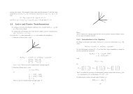
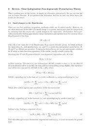
Section 12: Laplace Transforms12. 1. Laplace Transform as relative of Fourier TransformFor some simple functions the F.T. does not exist e.g. f(x) = x 2 since the integral diverges.The divergence at x = +∞ can be remedied by introducing a factor e −xγ , where R[γ]is sufficiently large and positive, into the integrand. However we then cause problems atx = −∞. But, for many dynamical problems (where we use t rather than x for the argument)we are only interested in the behaviour for t > 0 subject to some initial conditions at t = 0.We can thus consider f(t)e −γt θ(t) whose F.T. and inverse becomesg(ω) =∫ ∞f(t)e −γt θ(t) = 12π−∞∫ ∞dt f(t)e −γt θ(t)e −iωt =−∞g(ω)e iωt dω∫ ∞0dt f(t)e −(γ+iω)tNow let s = γ + iω, and rename g(ω) as F (s), then dropping the theta function (with theunderstanding that we consider t ≥ 0) we findF (s) =∫ ∞0f(t) = 12πidt f(t)e −st (1)∫ γ+i∞γ−i∞ds F (s)e st (2)(1) is the definition of the Laplace transform often denoted L[f(t)] and (2) is the inversionformula (sometimes known as the Bromwich inversion formula).In practice (1) will only converge for R[s] sufficently large. Consequently, the constant γ inthe inversion contour in (2) must be chosen to be to the right of any singularity of F (s) inthe complex s plane. For t > 0 the contour can be closed as a large semicircle to the left(which vanishes by a Jordan’s lemma argument)—see figure. One can then use the residuetheorem to obtain f(t) from F (s)52

12. 2. Simple examplesf(t) =t ν F (s) =∫ ∞f(t) =e ωt F (s) = 1s − ω0t ν e −st dt = 1 ∫ ∞u ν e −u du =s ν+1(s > ω)f(t) =e iωt F (s) = 1s − iω = s + iωs 2 + ω 2 (s > 0)f(t) = cos ωt F (s) =f(t) = sin ωt F (s) =0Γ(ν + 1)s ν+1 (s > 0)12(s 2 + ω 2 ) [s + iω + s − iω] = s(s > 0)s 2 + ω 2ws 2 + ω 2 (s > 0)f(t) =δ(t − a) F (s) = e −as (s > 0)f(t) =θ(t − a)F (s) = e−ass(s > 0)Denoting L[f(t)] = F (s) we also haveL[f ′ (t)] =∫ ∞0f ′ (t)e −st dt = [ f(t)e −st] ∫ ∞∞+ s f(t)e −st dt = sF (s) − f(0)0L[f ′′ (t)] =s 2 F (s) − sf(0) − f ′ (0)L[tf(t)] =∫ ∞0tf(t)e −st dt = − d ds L[f(t)]012. 3. Inversion of Laplace Transform1. ‘Engineering approach’ — just look up tables of known Laplace transforms, to workout what is the inverse of a given Laplace Transform2. Evaluate the inversion integral (2). This has the advantage of our really understandingwhere the result comes from plus it allows an easy evaluation of the large t behaviour(see later).Example: F (s) = 1/sWe have a simple pole at s = 0 thusso f(t) = θ(t)Example: F (s) = 1/s m+1 m integerWe have pole of order m + 1 at s = 0 thusfor t > 0 f(t) = Residue of e st /s = 1for t > 0 f(t) = Residue of e st /s m+1 = tm m!53

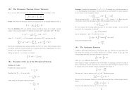
Figure 1: Bromwich Inversion integral; γ is to right of any singularity of F (s); for t > 0 weclose contour to the left(where to obtain the residue we Taylor expand the exponential) and so f(t) = tm m! θ(t)12. 4. Solution of ODEs with initial conditionsAs our canonical example we considerü(t) + 2κ ˙u + ω 2 0 = 0 u(0) = u 0 ˙u(0) = v 0Take the Laplace transform and use results of 14.2s 2 F (s) − su(0) − ˙u(0) + 2κ[sF (s) − u(0)] + ω 2 0F (s) = 0Now we have to invert F (s).⇒ F (s) = (s + 2κ)u 0 + v 0(s + κ) 2 + ω 2 where ω 2 ≡ ω 2 0 − κ 2We can use (i) the engineering approach and look up tables e.g. standard Laplace transforms—which you should check—areL[e −κt cos ωt] =s + κ(s + κ) 2 + ω 2 L[e −κt sin ωt] =ω(s + κ) 2 + ω 2Or (ii) we can use the inversion integral (2), which we choose to do here.u(t) = 12πi∫ γ+i∞γ−i∞ds [(s + 2κ)u 0 + v 0 ](s − s + )(s − s − ) est s ± = −κ ± iωThus we have two simple poles at s = s ± within the contour (for t > 0 closed by largesemicircle to left) and we can evaluate the sum of the residuesu(t) = [(s + + 2κ)u 0 + v 0 ](s + − s − )= e−κtωe s +t + [(s − + 2κ)u 0 + v 0 ]e s −t(s − − s + )[(κu o + v 0 ) sin ωt + ωu 0 cos ωt]54

12. 5. ConvolutionIn the context of Laplace transforms we define the convolution asf(t) ◦ g(t) =∫ t0f(t − z)g(z)dzi.e. the limits come from the restriction that the arguments of the two functions be positive.L[f(t) ◦ g(t)] =One can also show==∫ ∞0∫ ∞0∫ ∞0∫ tdte −st dz f(t − z)g(z)dzdz= L[f]L[g]0∫ ∞z∫ ∞0L[f 1 f 2 ] = 12πidt e −st f(t − z)g(z)du e −s(u+z) f(u)g(z) where u = t − z∫ γ+i∞γ−i∞F 1 (z)F 2 (s − z)dzwhere F 1 , F 2 are Laplace transforms of f 1 , f 2 respectively. If F 1 (s), F 2 (s) exist for R[s] > α 1 ,R[s] > α 2 respectively, we need R[s] − α 2 > γ > α 1 .Example: Forced, damped, harmonic motionẍ + 2κẋ + ω 2 0x = f(t) x(0) = 0 ẋ(0) = 0Then denote L.T. of x(t), f(t) by ˜x(s), ˜f(s). We find (see 14.4)˜x(s) =⇒ x =where G(u) = 12πi1(s + κ) 2 + ω ˜f(s) 2∫ ∞0∫ γ+i∞γ−i∞G(t − t ′ )f(t ′ )dt ′e suds(s + κ) 2 + ω = 1 2 ω e−κu sin ωu Θ(u)55

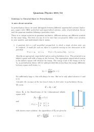
Section 12cont: More on Laplace Transforms12. 6. Integral representationsThe inversion integral can often be used to develop integral representations of special functions.For example in 14.2 we saw L[t ν Γ(ν + 1)] = . Thuss ν+1L −1 [ 1s ν+1 ]=Then using the inversion integral this becomest νΓ(ν + 1) = 12πit νΓ(ν + 1) .∫ γ+i∞γ−i∞ds ests ν+1where γ > 0 so that we are to the right of the singularity at s = 0 which is a branch point forν noninteger. We take the branch cut along the negative real axis. Then (see figure) whenwe close the contour to the left we have to avoid the branch cut. Thus a closed contour thatencircles no singularities is C I + C II + C III + C where C I is the Bromwich contour (parallelto the imaginary axis); C II , C III are quarter circles going from γ + i∞ to −∞ and from−∞ to γ − i∞; C is a ‘loop’ or ‘Hankel type’ contour that comes in from −∞ just abovethe branch cut, encircles the origin and goes out to −∞ just below the branch cut (similarto the contour we have used for Bessel functions of noninteger order). We may show thatthe integrals along C II and C III tend to zero —let s = γ + iz then the integrals wrt z vanishby a Jordan’s Lemma argument. Since the closed contour gives 0 our Bromwich integral isequal to the integral along the contour −C.Figure 2: Closing the inversion contour, and the Hankel type contour C for F (s) = 1/s ν+11Γ(ν + 1)= t −ν 1 ∫2πi Cdss ν+1 est = 1 ∫dz e z z −ν−1 (z = st) .2πi CThus we have found an integral representation of Γ −1 (ν + 1). This integral representationcan be verified by setting z = e iπ u above and z = e −iπ u below the branch cut. One thenidentifies the u integral as Γ(−ν) and invokes Euler’s reflection formula to get the result(exercise).56

12. 7. Coupled equationsTo illustrate the power of Laplace transforms let us consider a set of coupled first-order ODEdN 1dtwith initial condition= −λ 1 N 1dN 2dt= λ 1 N 1 − λ 2 N 2dN 3dt= λ 2 N 2 − λ 3 N 3 (3)N 1 (0) = N N 2 (0) = 0 N 3 (0) = n .This system of equation describes a chain of radioactive decay: species 1 decays to species2 which decays to species 3 which then decays to an inert product. N i is the number ofeach species. λ i are decay rates and are positive. Thus for example the equation for dN 2 /dtrepresents the increase in N 2 due to species 1 decaying and the decrease due to species 2decaying.We wish to find N i (t), in particular the long time behaviour of N 3 (t) for example.To begin we take Laplace transforms of (3) defining F 1 (s) as the L.T. of N 1 (t) etc:sF 1 (s) − N 1 (0) = −λ 1 F 1 (s)sF 2 (s) − N 2 (0) = λ 1 F 1 (s) − λ 2 F 2 (s)sF 3 (s) − N 3 (0) = λ 2 F 2 (s) − λ 3 F 3 (s)which imposing the initial conditions givesF 1 (s) =Ns + λ 1F 2 (s) = λ 1F 1 (s)s + λ 2=λ 1 N(s + λ 2 )(s + λ 1 )F 3 (s) =n F 2 (s)+ λ 2 = nλ 1 λ 2 N+s + λ 3 s + λ 3 s + λ 3 (s + λ 3 )(s + λ 2 )(s + λ 1 )To find N 3 (t) we could in this case invert the expression for F 3 (s) by using partial fractionsand the inverse transform L −1 [1/(s + λ i )] = e −λ it . However, to get a better understandingof what’s going on we use the inversion integralN 3 (t) = 12πi∫ γ+i∞γ−i∞ds F 3 (s)e stWe note that F 3 (s) has simple poles at s = −λ 1 , −λ 2 , −λ 3 thusN 3 = sum of residues=λ 1 λ 2 N(λ 3 − λ 1 )(λ 2 − λ 1 ) e−λ 1t +λ 1 λ 2 N(λ 3 − λ 2 )(λ 1 − λ 2 ) e−λ 2t +λ 1 λ 2 N(λ 2 − λ 3 )(λ 1 − λ 3 ) e−λ 3t + ne −λ 3tSince λ i > 0 the long time behaviour is clearly given by λ i with the smallest real part e.g. ifλ 1 < λ 2 , λ 3λ 1 λ 2 Nfor large t N 3 (t) ∼(λ 3 − λ 1 )(λ 2 − λ 1 ) e−λ 1t .Thus the long time behaviour is given by the pole of F (s) that is furthest to the right in thecomplex s plane.57

In the present example the intuitive explanation is that the chain of decays is limited by thestep with the slowest rate.Now let us try to generalise (3) by writing it as a matrix equation⎛⎞−λdN1 0 0dt = ⎝ λ 1 −λ 2 0 ⎠ N = MN (4)0 +λ 2 −λ 3Take the Laplace transform[sF (s) − N(0)] = MF (s) ⇒ F (s) = (s 1 − M) −1 N(0)where (s 1 − M) −1 is the inverse matrix of (s 1 − M). We can then invert the L.T. byN(t) =∫ γ+i∞γ−i∞ds (s 1 − M) −1 N(0)e stSo in principle we have to find the inverse of (s 1 − M).Now(s 1 − M) −1 =Matrix of cofactorsdet(s 1 − M)=Matrix of cofactors∏µ i(s − µ i )The last equality comes from the fact that the determinant of a matrix equals the productof its eigenvalues and the eigenvalues of s 1 − M are s − µ i where µ i are the eigenvalues ofM.Thus the singularities of F (s) are poles located at s = µ i the eigenvalues of the matrix M.Asymptotically (t large) the eigenvalue furthest to the right i.e. with the largest real partwill dominate. This is a very general result for equations of the from (4).N.B. we have assumed the matrix is diagonalisable and we have ignored any degeneracies.To check the general result we can return to our example (3) where indeed detM = −λ 1 λ 2 λ 3and the eigenvalues are −λ 1 , −λ 2 , −λ 3 .12. 8. Asymptotic behaviour t → ∞We have seen that if the singularities of F (s) are isolated poles or branch points then theinversion integral reduces to a sum of residues (from the poles) and ‘loop integrals’ aroundthe branch points (see example of 15.1).The contribution from a singularity at s 0 comes with a factor e s0t . Thus for large t thesingularity furthest to the right in the complex s plane (largest R[s 0 ]) dominatesFor poles it is straightforward to determine the residue (see e.g. 15.2).For branch points one has to do a little more work:The idea is to expand F (s) around the branch point at s 0 :F (s 0 ) ∼ ∑ νa ν (s − s 0 ) λνwhere this is generally an asymptotic expansion (for s − s 0 → 0) and λ ν may be non-integer58

Then a loop integral around the branch point at s 0 will usually result in an asymptotic seriesthat can be obtained integrating term by term∫1ds F (s)e st ∼ 1 ∫ds ∑ a ν (s − s 0 ) λν e st = e ∑ s a0t ν2πi C s02πi C s0Γ(−λνν ν )t λν+1Where we have used from 15.1.L −1 [s −ν ] =1Γ(−λ ν )t λν+1An interesting point is that we generate a power series that multiplies the exponential behaviourand when s 0 = 0 (which is often the case) the asymptotic behaviour is a power lawdecay.ExampleF (s) =1√s(s + a)a > 0This has branch points at s = 0, −a of which s = 0 is furthest to the right. Now expandF (s) about s = 0:F (s) = √ 1 1sa (1 + s/a) = 1 [√ 1 − s]1/2 sa 2a + 3s28a + · · · 2In this case the expansion is convergent i.e. it is s −1/2 A(s) where A(s) is a Taylor seriesconvergent for |s| < 1.We now inverse transform term by term:f(t) = √ 1 []1a Γ(1/2)t − 11/2 2aΓ(−1/2)t + 33/2 8a 2 Γ(−3/2)t + · · · 5/2Recalling Γ(z + 1) = zΓ(z) and Γ(1/2) = √ π we deduce Γ(−1/2) = −2 √ π, Γ(−3/2) =4 √ π/3. Thus we obtain an asymptotic expansion for large t as[1f(t) = √ 1 + 1πa t1/24at + 9 ]32a 2 t + · · · 212. 9. Other transform pairsFourier Transform g(k) =Laplace Transform F (s) =Mellin Transform φ(z) =Hilbert Transform∫ ∞−∞∫ ∞0∫ ∞0g(y) = 1 π P ∫ ∞dx f(x)e −ikx f(x) = 1 ∫ ∞dkg(k)e ikx2π −∞dt f(t)e −st f(t) = 12πidt f(t)t z−1 f(t) = 12πi−∞dx f(x)x − y∫ γ+i∞γ−i∞∫ c+i∞c−i∞f(x) = 1 π P ∫ ∞−∞ds F (s)e stdz φ(z)t −zdy g(y)y − xWhere P indicates the Cauchy principal value of the integral. The Mellin transform isparticularly useful for asymptotic expansions and is basically a Laplace transform with e −treplaced by t. It generally only exists in a strip e.g. α < R[z] < β.59