info document - Paris School of Economics

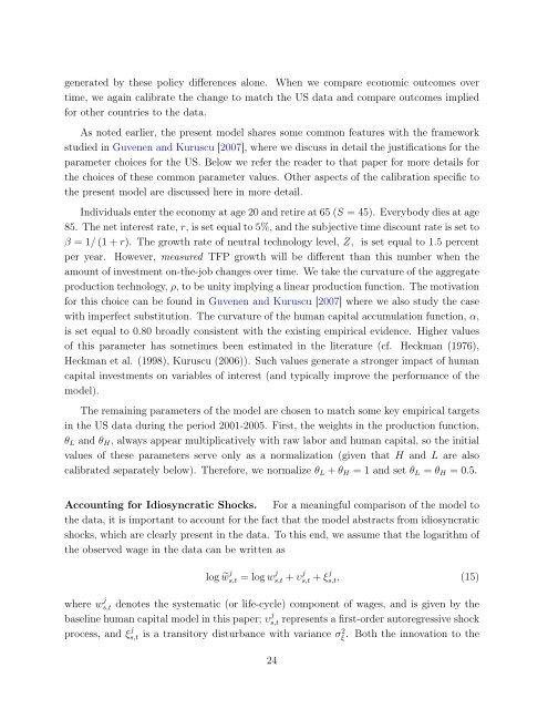
generated by these policy differences alone. When we compare economic outcomes overtime, we again calibrate the change to match the US data and compare outcomes impliedfor other countries to the data.As noted earlier, the present model shares some common features with the frameworkstudied in Guvenen and Kuruscu [2007], where we discuss in detail the justifications for theparameter choices for the US. Below we refer the reader to that paper for more details forthe choices of these common parameter values. Other aspects of the calibration specific tothe present model are discussed here in more detail.Individuals enter the economy at age 20 and retire at 65 (S = 45). Everybody dies at age85. The net interest rate, r, is set equal to 5%, and the subjective time discount rate is set toβ = 1/ (1 + r). The growth rate of neutral technology level, Z, is set equal to 1.5 percentper year. However, measured TFP growth will be different than this number when theamount of investment on-the-job changes over time. We take the curvature of the aggregateproduction technology, ρ, to be unity implying a linear production function. The motivationfor this choice can be found in Guvenen and Kuruscu [2007] where we also study the casewith imperfect substitution. The curvature of the human capital accumulation function, α,is set equal to 0.80 broadly consistent with the existing empirical evidence. Higher valuesof this parameter has sometimes been estimated in the literature (cf. Heckman (1976),Heckman et al. (1998), Kuruscu (2006)). Such values generate a stronger impact of humancapital investments on variables of interest (and typically improve the performance of themodel).The remaining parameters of the model are chosen to match some key empirical targetsin the US data during the period 2001-2005. First, the weights in the production function,θ L and θ H , always appear multiplicatively with raw labor and human capital, so the initialvalues of these parameters serve only as a normalization (given that H and L are alsocalibrated separately below). Therefore, we normalize θ L + θ H = 1 and set θ L = θ H = 0.5.Accounting for Idiosyncratic Shocks. For a meaningful comparison of the model tothe data, it is important to account for the fact that the model abstracts from idiosyncraticshocks, which are clearly present in the data. To this end, we assume that the logarithm ofthe observed wage in the data can be written aslog ˜w j s,t = log w j s,t + υ j s,t + ξ j s,t, (15)where w j s,t denotes the systematic (or life-cycle) component of wages, and is given by thebaseline human capital model in this paper; υ j s,t represents a first-order autoregressive shockprocess, and ξ j s,t is a transitory disturbance with variance σξ 2 . Both the innovation to the24