info document - Paris School of Economics

More documents

Recommendations

Info

for all cohorts. Each distribution is fully characterized by two parameters, giving us fourparameters to be calibrated. 12 The mean value of raw labor, E [l j ] , is a scaling parameterand is normalized to one, leaving three parameters: (i) the cross-sectional standard deviationof raw labor, σ (l j ) , (ii) the mean learning ability, E [A j ], and (iii) the dispersion inthe ability to learn, σ (A j ) . These are chosen to match the following three moments:1. the average cross-sectional variance of log wages between 1965 and 1969,2. the average level of the log college premium between 1965 and 1969,3. the mean log wage growth over the life cycle.As discussed above, we need an estimate of the variances συ 2 and σξ2 to obtain the targetvalue for the cross-sectional wage inequality. Note that, for consistency, these estimatesmust be obtained from empirical studies that allow for heterogeneity in wage growth ratesas implied by the human capital model in this paper. 13 Guvenen (2005) estimates such aspecification and reports σξ 2 to be 0.047. Similarly, σ2 υ can be calculated to be 0.088 usingthe estimates in that paper (Table 1, row 2). The average cross-sectional variance of logwages in the U.S. data between 1965 and 1969 is 0.239, implying a target value for the firstmoment in the model (var ( ws,t) j ) of 0.104. Second, the log college premium in the U.S.data averaged 0.381 between 1965 and 1969 (and does not require any adjustments), whichis the second empirical target we choose. Third, and finally, our target for mean log wagegrowth between ages 20 and 55 is 50 percent for a cohort of individuals who retire before1970. This number is roughly the middle point of the figures found in studies that estimatelife-cycle wage and income profiles from panel data sets such as the Panel Study of IncomeDynamics (which typically report estimates between 40 and 65 percent; see, for example,Gourinchas and Parker (2002), Davis, Kubler and Willen (2002), Guvenen (2005)). 1412 Notice that we also need to calibrate the cross-sectional correlation of l and A. Since we interpretthe heterogeneity in l as arising from investments made prior to college and high-ability individuals arelikely to have invested more even before college, it seems reasonable to conjecture that A and l will bepositively correlated. Indeed, Huggett et al (2006b) estimate the parameters of the standard Ben-Porathmodel from individual wage data allowing for heterogeneity in A and l, and provide evidence that the twoare strongly positively correlated (corr: 0.792). For simplicity we assume perfect correlation between thetwo. Furthermore, it will become clear later that the heterogeneity in l does not play a significant role inthis model, implying that the choice of perfect correlation is not likely to be critical.13 This requirement eliminates several well-known empirical papers, such as MaCurdy (1982), Abowd andCard (1989), and Meghir and Pistaferri (2004), among others, which restrict wage growth rates to be thesame across the population.14 Ideally, we would like to use an estimate of average life-cycle wage growth during the period before1970 (before SBTC), whereas PSID is only available starting 1968 on. However, we are not aware of anystudy that estimates the life-cycle (not cross-sectional) wage profiles using data from earlier periods. Ourcalibration implies a mean log wage growth of 62 percent for the cohort that enters the economy in 1968,consistent with the numbers found by these studies during the same period.26
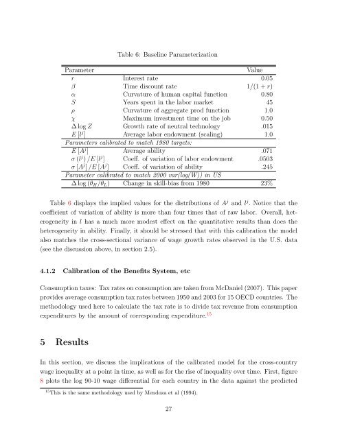
Table 6: Baseline ParameterizationParameterValuer Interest rate 0.05β Time discount rate 1/(1 + r)α Curvature of human capital function 0.80S Years spent in the labor market 45ρ Curvature of aggregate prod function 1.0χ Maximum investment time on the job 0.50∆ log Z Growth rate of neutral technology .015E [l j ] Average labor endowment (scaling) 1.0Parameters calibrated to match 1980 targets:E [A j ] Average ability .071σ (l j ) /E [l j ] Coeff. of variation of labor endowment .0503σ [A j ] /E [A j ] Coeff. of variation of ability .245Parameter calibrated to match 2000 var(log(W)) in US∆ log (θ H /θ L ) Change in skill-bias from 1980 23%Table 6 displays the implied values for the distributions of A j and l j . Notice that thecoefficient of variation of ability is more than four times that of raw labor. Overall, heterogeneityin l has a much more modest effect on the quantitative results than does theheterogeneity in ability. Finally, it should be stressed that with this calibration the modelalso matches the cross-sectional variance of wage growth rates observed in the U.S. data(see the discussion above, in section 2.5).4.1.2 Calibration of the Benefits System, etcConsumption taxes: Tax rates on consumption are taken from McDaniel (2007). This paperprovides average consumption tax rates between 1950 and 2003 for 15 OECD countries. Themethodology used here to calculate the tax rate is to divide tax revenue from consumptionexpenditures by the amount of corresponding expenditure. 155 ResultsIn this section, we discuss the implications of the calibrated model for the cross-countrywage inequality at a point in time, as well as for the rise of inequality over time. First, figure8 plots the log 90-10 wage differential for each country in the data against the predicted15 This is the same methodology used by Mendoza et al (1994).27
Page 3 and 4: Table 1: Log Wage Differential Betw
Page 5 and 6: of policies for wage inequality.The
Page 8 and 9: Table 3: Tax Function Parameter Est
Page 10 and 11: Figure 1: Estimated Average Tax Rat
Page 12 and 13: Table 4: Progressivity and Wage Ine
Page 14 and 15: Figure 4: Progressivity Wedge* and
Page 16 and 17: Figure 7: Change in Hours/Person an
Page 18 and 19: which is simply the forgone earning
Page 20 and 21: system, (ii) finance government exp
Page 22 and 23: 4. The government budget balances:
Page 24 and 25: generated by these policy differenc
Page 28 and 29: 1.61.51.4Figure 8: Wage Dispersion:
Page 30 and 31: Table 8: Contribution of Taxes to t
Page 32 and 33: ReferencesFatih Guvenen. An empiric

info document - Paris School of Economics

You also want an ePaper? Increase the reach of your titles

Delete template?

Save as template?