1 2D Continuous wavelet transform

2Dcwttools.tex Last compiled: Monday 22 nd January, 2007 15:331 2D Continuous wavelet transformWe extend the continuous wavelet transform (CWT) to two-dimensions.A 1D CWT is performed by convolving a wavelet function ψ(x) and signal f(x)˜f(a, b) = 1 √ a∫f(x)ψ( x − a )dx (1)bRotations are also included in the extension to higher dimensions. This can give thewavelet a sensitivity to direction.ψ l,x ′ ,θ(x) = l n/2 ψ[Ω −1 (θ) x − x′] (2)lwhere n = 2 is the number of dimensions of our physical space, l is the scale of thewavelet, x ′ is the position, and θ is the angle of the wavelet (like a polarization) and Ω(θthe rotation matrix operator. The CWT becomes∫f(l, x ′ , θ) =< ψ l,x ′ ,θ|f >= ψl,x ∗ ,θ(x)d n x (3)′R nA wavelet in higher dimensions must still satisfy the admissibility conditionwhere n = 2 in the 2D case.C ψ = (2π) 2 ∫ | ˆψ(k)|21.1 Complex Morlet wavelet|k| n dn k < ∞ (4)Here we take the 2D complex Morlet wavelet as a plane wave modulated by a Gaussianenvelope.ψ(x) = e ik ψ·x e − 1 2 |x|2 (5)where the parameter k ψ is the wavenumber associated with the Morlet wavelet.To take the 2D Fourier transform∫ˆf(k) = f(x)e ik·x dx (6)∫ ∫ˆf(k x , k y ) =f(x, y)e ikxx e ikyy dxdy (7)where k x and k y are the components of the wave vector.The Fourier transform of the 2D complex Morlet wavelet (uncorrected) isequivalent toˆψ(k) = 2πe −(kx−k ψ) 2 /2 e −k2 y /2 (8)ˆψ(k) = 2πe k ψ·k e −|k|2 /2 e −|k ψ| 2 (9)1

2Dcwttools.tex Last compiled: Monday 22 nd January, 2007 15:33As one can see, this is not zero at k = 0. Strictly speaking, this formula does notsatisfy the admissibility condition for a wavelet (roughly speaking it does not have a zeromean). We can either enforce the admissibility by setting ˆψ(k = 0) = 0 1 or by makinga correction to the formula to satisfy the admissibility condition. We use the analyticcorrection so that the resulting zero mean formula for the complex Morlet wavelet becomesψ(x, y) = (e ik ψx − e − 1 2 k2 ψ )e− 1 2 (x2 +y 2 )(10)The correction factor e − 1 2 k2 ψ is small, but not always negligible (depending on the valueof k ψ ). I prefer to use the correction, as it is not ad hoc and does not complicate thingstoo much. The Fourier transform of the corrected complex Morlet wavelet isso thatˆψ(k) = √ 2π[e − 1 2 (2πk−k ψ) 2 − e − 1 2 k ψ 2 e − 1 2 (2πk)2 ] (11)ψ(k x , k y ) = √ 2π[e − 1 2 (2πkx−k ψ) 2 +(2πk y) 2 − e − 1 2 k2 ψ e− 1 2 (2πk2 x+2πk 2 y] (12)Note that in Fourier space the correction rapidly decreases away from the |k| = 0origin. For the wavelet at a given dilation a, its frequency centered at k = k ψ /2πa where∫ ∞k| ˆψ(k)|dk0k ψ = ∫ ∞| ˆψ(k)|dk(13)0Is the barycenter of the wavelet in Fourier space.It is important to find the correspondence between the dilation parameter a and thescale of the wavelet. We first find the relation between the central frequency of the waveletand the dilation parameter a.The calculus involved in calculating k ψ for the complex Morlet wavelet is a bit messy,but the result is clean and should be obvious. For the complex Morlet waveletk ψ = k ψ (14)A result we should recognize as obvious, since this is what we put into the wavelet.We empirically set the length scale of the complex Morlet l = 1 at value of dilationparameter a = 0.1329. Therefore to convert between the scale of the Morlet l, basedupon the domain size, and the dilation parameter, a = 0.1329l. Therefore to convert towavenumberk ψk =(15)(2π(0.1329)l).We also include rotations. Rotations can be included in the extension to higherdimensions. This can give the wavelet a sensitivity to direction.ψ l,x ′ ,θ(x) = l n/2 ψ[Ω −1 (θ) x − x′] (16)l1 Note that in Matlab the DC mode is stored at the first index of the matrix resulting from the fft2function. I.e. if Y = fft2(X); then Y(1,1) = sum(sum(X)); is the DC mode.2

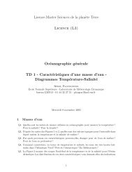
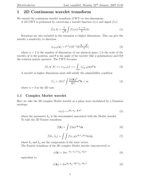
2Dcwttools.tex Last compiled: Monday 22 nd January, 2007 15:33where n = 2 is the number of dimensions of our physical space, l is the scale of thewavelet, x ′ is the position, and θ is the angle of the wavelet (like a polarization) and Ω(θ)the rotation matrix operator.Note that rotations have the same effect whether in physical or in spectral space. Werotate the domain of the computation to rotate the wavelet, so thatin physical space, and equivalentlyx ↦→ x cos(θ) + y sin(θ) (17)y ↦→ y cos(θ) − x sin(θ) (18)k x ↦→ k x cos(θ) + k y sin(θ) (19)k y ↦→ k y cos(θ) − k x sin(θ) (20)in spectral space.Examples of the 2D complex Morlet for different scales, fixed at k ψ = 6 are shownin figures 1,2, 3, and 4, for scales l = 1.0, 0.5, 0.2, and 0.1, respectively. Included inthe figures are representations of the wavelets at several different angles. The Fourierspacerepresentations are calculated from the physical space formula using Matlab’s FFTalgorithm and are displayed with the zero-frequency in the center by using Matlab’sfftshift function.1.2 Calculation of the phaseHere we describe the calculation of the phase of wavelet coefficients and problems withthe calculation.For continuous wavelet transformations with complex wavelets we can calculate thephase from the real and imaginary parts of the wavelet coefficients.Θ = arctan ( I ˜f ) (21)R ˜fWe want to define the phase as varying from [0, 2π] where Θ = 0 and Θ = 2πcorresponds to the semi-axis where I = 0 and R > 0. Therefore there is a discontinuityin the phase. This creates a problem where the imaginary component of the waveletcoefficients are very small (i.e. order of the computer roundoff).An example of the problem encountered by taking the CWT of a dirac function isshown in figure ??. A cut through the phase and coefficients where the discontinuities inthe phase occurs is show in figure ??.The solution to this is perhaps to define the phase to vary from 0

2Dcwttools.tex Last compiled: Monday 22 nd January, 2007 15:33scale = 1; ! = 0scale = 1; ! = 00.40.30.20.1642100500.80.70.60.5y0!0.1!0.2!0.3!0.4!0.5!0.4 !0.2 0 0.2 0.4x0!2!4!6k y0!50!100!100 !50 0 50 100k x0.40.30.20.1scale = 1; ! = pi3scale = 1; ! = pi30.40.30.20.1642100500.70.60.5y0!0.1!0.2!0.3!0.4!0.5!0.4 !0.2 0 0.2 0.4x0!2!4!6k y0!50!100!100 !50 0 50 100k x0.40.30.20.1scale = 1; ! = 3pi2scale = 1; ! = 3pi20.40.30.20.1642100500.80.70.60.5y0!0.1!0.2!0.3!0.4!0.5!0.4 !0.2 0 0.2 0.4x0!2!4!6k y0!50!100!100 !50 0 50 100k x0.40.30.20.1Figure 1: Complex Morlet wavelet at scale = 1.0. The left column is the real part ofthe wavelet in physical space, the right column is the modulus of the wavelet in spectralspace. The rows from top down correspond to rotations of θ = 0, π/3, and 3π/2. Thearrow indicates the direction of the wavelet.4

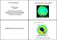
2Dcwttools.tex Last compiled: Monday 22 nd January, 2007 15:33scale = 0.5; ! = 0scale = 0.5; ! = 00.40.3101000.40.350.20.15500.30.25y0!0.1!0.2!0.3!0.40!5!10k y0!50!1000.20.150.10.05!0.5!0.4 !0.2 0 0.2 0.4x!100 !50 0 50 100k x0.40.3scale = 0.5; ! = pi310100scale = 0.5; ! = pi30.40.350.20.15500.30.25y0!0.1!0.2!0.3!0.40!5!10k y0!50!1000.20.150.10.05!0.5!0.4 !0.2 0 0.2 0.4x!100 !50 0 50 100k xscale = 0.5; ! = 3pi2scale = 0.5; ! = 3pi20.40.3101000.40.350.20.15500.30.25y0!0.1!0.2!0.3!0.40!5!10k y0!50!1000.20.150.10.05!0.5!0.4 !0.2 0 0.2 0.4x!100 !50 0 50 100k xFigure 2: Complex Morlet wavelet at scale = 0.5. The left column is the real part ofthe wavelet in physical space, the right column is the modulus of the wavelet in spectralspace. The rows from top down correspond to rotations of θ = 0, π/3, and 3π/2. Thearrow indicates the direction of the wavelet.5

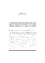
2Dcwttools.tex Last compiled: Monday 22 nd January, 2007 15:33scale = 0.2; ! = 0scale = 0.2; ! = 00.40.30.23020100500.160.140.120.1100.1y0!0.1!0.2!0.3!0.40!10!20k y0!50!1000.080.060.040.02!0.5!0.4 !0.2 0 0.2 0.4x!100 !50 0 50 100k xscale = 0.2; ! = pi3scale = 0.2; ! = pi30.40.30.20.1302010100500.160.140.120.1y0!0.1!0.2!0.3!0.4!0.5!0.4 !0.2 0 0.2 0.4x0!10!20!30k y0!50!100!100 !50 0 50 100k x0.080.060.040.02scale = 0.2; ! = 3pi2scale = 0.2; ! = 3pi20.40.30.23020100500.160.140.120.1100.1y0!0.1!0.2!0.3!0.40!10!20k y0!50!1000.080.060.040.02!0.5!0.4 !0.2 0 0.2 0.4x!100 !50 0 50 100k xFigure 3: Complex Morlet wavelet at scale = 0.2. The left column is the real part ofthe wavelet in physical space, the right column is the modulus of the wavelet in spectralspace. The rows from top down correspond to rotations of θ = 0, π/3, and 3π/2. Thearrow indicates the direction of the wavelet.6

2Dcwttools.tex Last compiled: Monday 22 nd January, 2007 15:33Matlab’s atan function returns an angle that is defined from [−π/2, π/2]. Becausethe argument is the ratio of the imaginary and real components, the function can notdistinguish between phase angles where the sign of the real and imaginary components areswapped. Matlab’s atan2 function accepts as inputs the imaginary and real componentsand can distinguish the full 2π angle of phase. However the result from atan2 is definedon the [−π, π] interval. We must therefore adjust the result to fit onto the [0, 2π] interval.1.3 Analysis and diagnosticsHere we list some diagnostic tools that we can calculate from the coefficients of the wavelettransform [?] (repeat of annual review).1.3.1 Energy diagnosticsThe first is the space-scale energy density (proposed by Moret-Bailly et al 1991)E(l, x) = | ˜f(l, x)| 2(22)l nwhich can be integrated over scale to obtain the local energy density∫ ∞E(x) = C −1ψE(l, x) dl(23)0 l+Instead of integrating over scale, we can integrate over space to obtain the globalwavelet energy spectrum (a function of scale)∫E(l) = E(l, x)d n x (24)R nwhich is related to the Fourier energy spectrum∫E(l) = E(k)| ˆψ(lk)| 2 d n k (25)R nwhich is equivalent to the Fourier energy spectrum of the signal smoothed by thewavelet Fourier energy spectrum (E(k) = | ˆf(k| 2 ).We can recover the total energy of the signal by integrating over scaleE = C −1ψ∫ ∞E(l) dl0 l+(26)1.3.2 Local intermittency factorThe local intermittency factor measures the spatially local deviation from the Fourierenergy spectrum (or the global energy spectrum?? wavelet energy spectrum averagedover position) at a given scale.I(l, x) =| ˜f(l, x)| 2< | ˜f(l, x)| 2 > x(27)8

2Dcwttools.tex Last compiled: Monday 22 nd January, 2007 15:33Signals where I(l, x) = 1 have energy distributed evenly in space. Regions of signalswhere the intermittency factor is much greater than 1 correspond to intermittent features.(presumably these intermittent features will correspond to the coherent structures!)1.3.3 Local Reynolds numberFor a signal that corresponds to a turbulent flow we can construct the Reynolds numberRe as the non-dimensional ratio of the nonlinear advection terms to the linear viscousterms in the Navier-Stokes equations. This gives the level of nonlinearity of the flowand is a measure of the intensity of turbulence (i.e. Re ≫ 1 is generally turbulent,though depending upon the specifics flow, and is indicative of the range of scales ofmotion excited). A global Reynolds number, based upon characteristics of the flow, canbe estimated asRe = UL(28)νwhere U is a characteristic velocity scale (i.e the RMS turbulent velocity), L a characteristiclength scale, and ν the kinematic viscosity of the flow. We can construct theequivalent from the wavelet coefficients. A space-scale Reynolds number (Farge et al1990)ṽ(l, x)lRe(l, x) = (29)νwhere ṽ(l, x) is the characteristic RMS velocity that can be calculated by summingover the CWT of the various components of the velocity. i.e. in 3Dṽ(l, x) = [(3C ψ ) −13∑|ṽ n (l, x)| 2 ] −1/2 (30)n=1One can recover a local (in scale) Reynolds number by integrating over space∫Re(l) = Re(l, x)d n x (31)R n...global flow intermittency1.3.4 Local Rossby numbersHere I propose a measure of the local Rossby number for a rotating turbulent flow. TheRossby number Ro is a non-dimensional parameter based upon the ratio of the nonlinearterms to the Coriolis term in the Navier-Stokes equations with rotation. There are twoglobal Rossby numbers that one can construct. One is based upon the advection termRo =U(32)2ΩLwhere U is a characteristic velocity scale, 2Ω is the background vorticity (the rotationof the system), and L is a characteristic length scale of the flow. Another Rossby numbercan be constructed from the nonlinear term containing the time derivative of the velocity.9

2Dcwttools.tex Last compiled: Monday 22 nd January, 2007 15:33Ro = ω(33)2Ωis the Rossby number based upon the flow vorticity, and gives a ratio of the timescalesof structures in the flow to the background rotation rate. It can either be calculated fromthe global rms value (averaged over space) or the local rms value. We can constructtwo space-scale Rossby numbers from the wavelet coefficients in the same way that weconstructed the space-scale Reynolds number. The first based upon the CWT of thevelocityṽ(l, x)Ro u (l, x) = (34)2Ωlwhere ṽ(l, x) is the same RMS velocity used as in the local space-scale Reynoldsnumber calculation. The second Rossby number based upon the CWT of the vorticitywhere in 3DRo ω (l, x) =˜ω(l, x)2Ω(35)˜ω(l, x) = [(3C ψ ) −11.3.5 Space-scale contrastA contrast measure3∑|˜ω n (l, x)| 2 ] −1/2 (36)n=1where ¯f is defined asC(l, x) = | ˜f(l, x)| 2| ¯f| 2 (37)∫ l ′ =l¯f(l, x) = C −1ψ l−(n+1) ˜f(l ′ , x)dl ′ (38)l ′ =0 +is like the scaling function of the discrete wavelet transform.10