Variational Wavefunction for the Helium Atom

Technische Universität GrazInstitut für FestkörperphysikStudent projectVariational Wavefunctionfor the Helium AtomMolecular and Solid State Physics 513.001submitted on: 30. November 2009by:Markus Krammer

Contents1 Problem 32 Optimization of a given wavefunction 33 Calculating the energy E (α) 33.1 〈x|Ĥ|ψ〉 . . . . . . . . . . . . . . . . . . . . . . . . . . . . . . . . . . . . . . . . . . . . . . . . . . 33.2 〈ψ|Ĥ|ψ〉 . . . . . . . . . . . . . . . . . . . . . . . . . . . . . . . . . . . . . . . . . . . . . . . . . . 43.3 〈ψ|Ĥ1|ψ〉 . . . . . . . . . . . . . . . . . . . . . . . . . . . . . . . . . . . . . . . . . . . . . . . . . 43.4 〈ψ|ψ〉 . . . . . . . . . . . . . . . . . . . . . . . . . . . . . . . . . . . . . . . . . . . . . . . . . . . 53.5 〈ψ|Ĥ2|ψ〉 . . . . . . . . . . . . . . . . . . . . . . . . . . . . . . . . . . . . . . . . . . . . . . . . . 53.5.1 Transforming to spherical coordinates . . . . . . . . . . . . . . . . . . . . . . . . . . . . . 53.5.2 Determinant of the Jacobi matrix . . . . . . . . . . . . . . . . . . . . . . . . . . . . . . . . 73.5.3 One more transformation . . . . . . . . . . . . . . . . . . . . . . . . . . . . . . . . . . . . 93.5.4 Solving the integral . . . . . . . . . . . . . . . . . . . . . . . . . . . . . . . . . . . . . . . 94 Optimizing the Energy 102

1 ProblemThe Hamitonian for the helium atom isĤ = − 2 (∇22m 1 + ∇ 2 2e2) 2− −4πɛ 0 r 12e24πɛ 0 r 2+e24πɛ 0 r 12(1)where r 12 is the distance between the two electrons.There is no analytical solution for the Schrödinger equation for this problem. So in a first step we neglect theelectron electron interaction (term 5 in equation 1) to get an idea of how the real wavefunction could look like.Solving the Schrödinger equation for this simplified problem leads to the following wavefunction for the groundstate:ψ (r 1 , r 2 ) = 1 (a 3 exp −2 r )1 + r 2(2)0a 0This approximation is, of course, not very good. But it gives us an idea of how a better approximation couldlook like. So we try a variational wavefunction:ψ (r 1 , r 2 , α) = 1 (a 3 exp −α r )1 + r 2(3)0a 0Now, as we have made a decision of how our approximate wavefunction for the ground state should look like,we can optimize it.2 Optimization of a given wavefunctionTo optimize a wavefunction, we have to calculate the energyE (α) = 〈ψ|Ĥ|ψ〉〈ψ|ψ〉(4)and find the lowest energy depending on our parameter. If we would have more than one Parameter (e.g.coefficients of a polynomial that we multiply with our wavefunction) we would have to find the global minimumof our energy. But since we have just one parameter, finding the minimum energy is pretty easy.dE (α)dα = 0 (5)Equation 5 gives us the optimized parameter α (Energy must be the global minimum for the best α, so we haveto check whether this energy is the global minimum or not).3 Calculating the energy E (α)3.1 〈x|Ĥ|ψ〉The Laplace operator in spherical coordinates looks like this:∇ 2 i = 1 ( )∂ri2 ri2 ∂ 1 ∂ ∂ 1 ∂ 2+∂r i ∂r i ri 2 sin θ sin θ i +i ∂θ i ∂θ i ri 2 sin2 θ i ∂ϕ 2 i(6)Now we let the Laplace operator sink on the wavefunction:∇ 2 i ψ = 1 (∂ri2 r 2 ∂ 1i∂r i ∂r i a 3 exp −α r )1 + r 20a 0∇ 2 i ψ = − α a 4 01r 2 i(∂ri 2 exp −α r )1 + r 2∂r i a 0∇ 2 i ψ = − α a 4 01r 2 i( (2r i exp −α r )1 + r 2− α (ri 2 exp −α r ))1 + r 2a 0 a 0 a 03

∇ 2 i ψ = α a 4 0( α− 2 ) (exp −α r )1 + r 2a 0 r i a 0(7)Putting this into 〈x|Ĥ|ψ〉 returns:with〈x|Ĥ|ψ〉 = ( 2∑i=1(− 2(α α− 2 ) ) )−2e2 + e22m a 0 a 0 r i 4πɛ 0 r i 4πɛ 0 r 121a 3 0(exp −α r )1 + r 2a 0 2=e2(8)ma 0 4πɛ 0this leads to〈x|Ĥ|ψ〉 =2ma 4 0( 2∑ (− α2− 2 − α ) )+ 1 (exp −α r )1 + r 22ai=1 0 r i r 12 a 0(9)3.2 〈ψ|Ĥ|ψ〉With equation 9 it is not difficult to write down 〈ψ|Ĥ|ψ〉:〈ψ|Ĥ|ψ〉 =∫( 2∑· · · dx 1 dy 1 dz 1 dx 2 dy 2 dz 2∫R 2 (− α2− 2 − α ) )+ 1ma 6 0 2ai=1 0 r i r 121a 6 0(exp −2α r )1 + r 2a 0The first four terms in this integral are no problem to solve. Only the last term with the r 12 is a bit harder toevaluate. So we split it up into two parts:∫( 2∑〈ψ|Ĥ1|ψ〉 = · · · dx 1 dy 1 dz 1 dx 2 dy 2 dz 2∫R 2 (ma 7 − α2− 2 − α ) ) (exp −2α r )1 + r 2(11)6 0 2ai=1 0 r ia 0(10)and∫〈ψ|Ĥ2|ψ〉 =· · · dx 1 dy 1 dz 1 dx 2 dy 2 dz 2∫R 2 (1ma 7 exp −2α r )1 + r 26 0 r 12 a 0(12)3.3 〈ψ|Ĥ1|ψ〉The integrals∫· · · dx 1 dy 1 dz 1 dx 2 dy 2 dz 2∫R 2ma 7 6 0(− α2− 2 − α ) (exp −2α r )1 + r 22a 0 r 1 a 0and∫· · · dx 1 dy 1 dz 1 dx 2 dy 2 dz 2∫R 2 (− α2ma 7 − 2 − α ) (exp −2α r )1 + r 26 0 2a 0 r 2 a 0are exactly the same, so we can write∫〈ψ|Ĥ1|ψ〉 =· · · dx 1 dy 1 dz 1 dx 2 dy 2 dz 2∫R 2ma 7 6 0(− α2− 2 2 − α ) (exp −2α r )1 + r 2a 0 r 1 a 0(13)Now we tansform it into spherical coordinates and with the Jacobi determinant of the transformation we get:dx 1 dy 1 dz 1 dx 2 dy 2 dz 2 = r1 2 sin θ 1 r2 2 sin θ 2 dr 1 dϕ 1 dθ 1 dr 2 dϕ 2 dθ 2 (14)Our integral does not depend on ϕ i and θ i , so we can integrate these 4 variables seperately:∫ 2π∫ π ∫ 2π ∫ πdϕ 1 dθ 1 dϕ 2 dθ 2 sin θ 1 sin θ 2 = (4π) 2 (15)0 0 0 04

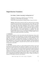
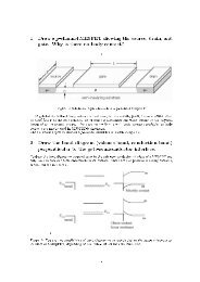
Figure 1: Transformation, the ˜z axis has the same direction as ⃗r 1and ˜z 2 as we are used to.˜x 2 = r 2 cos ϕ 12 sin θ 12 (24)ỹ 2 = r 2 sin ϕ 12 sin θ 12 (25)˜z 2 = r 2 cos θ 12 (26)So now we need to know the relation between x 2 , y 2 , z 2 and ˜x 2 , ỹ 2 , ˜z 2 . For this we write down the basis vectors:ê˜z = ⃗r 1r 1ê˜z =⎛⎝ cos ϕ 1 sin θ 1sin ϕ 1 sin θ 1cos θ 1⎞⎠ (27)êỹ = ê˜z × ê z|ê˜z × ê z |êỹ =⎛1⎝|ê˜z × ê z |cos ϕ 1 sin θ 1sin ϕ 1 sin θ 1cos θ 1⎞⎛⎠ × ⎝001⎞⎠êỹ =⎛1⎝|ê˜z × ê z |sin ϕ 1 sin θ 1− cos ϕ 1 sin θ 10⎞⎠6

where ˜M 1 , ˜M2 , ˜M3 and M are the more complicate parts of the Jacobi matrix with the transformation to r 2 ,ϕ 12 and θ 12 .∣ ∣∣∣∣∣∣∣∣∣ r 1 cos ϕ 1 sin θ 1 r 1 sin ϕ 1 cos θ 1˜M20 −r 1 sin θ 1˜M3|J| = cos ϕ 1 sin θ 1 0 00 0 M0 0∣∣ ∣∣∣∣∣∣∣∣∣ −r 1 sin ϕ 1 sin θ 1 r 1 cos ϕ 1 cos θ 1˜M10 −r 1 sin θ 1˜M3− sin ϕ 1 sin θ 1 0 00 0 M0 0∣∣ ∣∣∣∣∣∣∣∣∣ −r 1 sin ϕ 1 sin θ 1 r 1 cos ϕ 1 cos θ 1˜M1r 1 cos ϕ 1 sin θ 1 r 1 sin ϕ 1 cos θ 1˜M2+ cos θ 1 0 00 0 M0 0∣∣ ∣∣∣∣∣∣∣ −r 1 sin θ 1˜M3|J| = r 1 cos 2 ϕ 1 sin 2 0θ 10 M0∣ ∣∣∣∣∣∣∣ −r 1 sin θ 1˜M3r 1 sin 2 ϕ 1 sin 2 0θ 10 M0∣ ∣∣∣∣∣∣∣ r 1 sin ϕ 1 cos θ 1˜M20−r 1 sin ϕ 1 sin θ 1 cos θ 10 M0∣ ∣∣∣∣∣∣∣ r 1 cos ϕ 1 cos θ 1˜M10−r 1 cos ϕ 1 sin θ 1 cos θ 10 M0∣∣∣∣|J| = −r 2 1 sin 3 θ 1 |M| − r 2 1 sin 2 ϕ 1 sin θ 1 cos 2 θ 1 |M| − r 2 1 cos 2 ϕ 1 sin θ 1 cos 2 θ 1 |M|For the integral transformation we need the absolute value of the determinant of the Jacobi matrix.||J|| = r 2 1 sin θ 1 ||M|| (32)So now we just need to calculate the absolute value of the determinant of M:⎛ ⎞x 2 ( )M = ⎝ y 2⎠ · ∂ ∂ ∂∂r 2 ∂ϕ 12 ∂θ 12z 2M =⎛⎝ − cos ϕ ⎞ ⎛1 cos θ 1 sin ϕ 1 cos ϕ 1 sin θ 1− sin ϕ 1 cos θ 1 − cos ϕ 1 sin ϕ 1 sin θ 1⎠ ⎝ ˜x 2ỹ 2sin θ 1 0 cos θ 1 ˜z 2⎞⎠ ·(∂∂r 2∂∂ϕ 12)∂∂θ 12As the transformation matrix has no dependence on r 2 , ϕ 12 and θ 12 we can easily get the determinante:⎛⎞ ⎛ ⎞− cos ϕ 1 cos θ 1 sin ϕ 1 cos ϕ 1 sin θ 1 ˜x 2 ( ) ∣ |M| =⎝− sin ϕ 1 cos θ 1 − cos ϕ 1 sin ϕ 1 sin θ 1⎠ ⎝ ỹ 2⎠ · ∂ ∂ ∂ ∣∣∣∣∂r 2 ∂ϕ 12 ∂θ 12∣ sin θ 1 0 cos θ 1 ˜z 28

|M| =∣∣ ∣⎛− cos ϕ 1 cos θ 1 sin ϕ 1 cos ϕ 1 sin θ 1 ∣∣∣∣∣ ∣∣∣∣∣− sin ϕ 1 cos θ 1 − cos ϕ 1 sin ϕ 1 sin θ 1⎝sin θ 1 0 cos θ 1˜x 2ỹ 2˜z 2⎞⎠ ·(∂∂r 2∂∂ϕ 12∂∂θ 12) ∣ ∣ ∣∣∣∣The determinante of the second part is the same as we were calculating many times bevor:⎛⎝ ˜x ⎞2 ( ) ∣ ỹ 2⎠ · ∂ ∂ ∂ ∣∣∣∣∂r 2 ∂ϕ 12 ∂θ 12= −r2 2 sin θ 12∣ ˜z 2And the first part is also not really difficult:∣ − cos ϕ 1 cos θ 1 sin ϕ 1 cos ϕ 1 sin θ 1 ∣∣∣∣∣ − sin ϕ 1 cos θ 1 − cos ϕ 1 sin ϕ 1 sin θ 1 = cos 2 ϕ 1 cos 2 θ 1 +sin 2 ϕ 1 sin 2 θ 1 +cos 2 ϕ 1 sin 2 θ 1 +sin 2 ϕ 1 cos 2 θ 1 = 1∣ sin θ 1 0 cos θ 1So the absolute value of the determinante of the Jacobi matrix is:||J|| = r 2 1r 2 2 sin θ 1 sin θ 12 (33)3.5.3 One more transformationWith the transformation done before the integral is still not easy to solve. So we need one more transformation.We transform θ 12 to r 12 :r 2 12 = r 2 1 + r 2 2 − 2r 1 r 2 cos θ 12The Jacobi matrix for this transformation is:1 0 0 0 0 00 1 0 0 0 0|J| =0 0 1 0 0 00 0 0 1 0 00 0 0 0 1 0∣ r 12rr 1−r 2 cos θ 120 012r 2−r 1 cos θ 120r 12r 1r 2 sin θ 12∣ ∣∣∣∣∣∣∣∣∣∣∣||J|| =r 12r 1 r 2 sin θ 12(34)We need to take a look at the integration limits. In spherical coordinates they were the same as we are usedto. But now we have to get the correct limits for r 12 . The limits for θ 12 were 0 and π, so r 12 now needs to gofrom |r 1 − r 2 | to r 1 + r 2 .3.5.4 Solving the integralWith all these transformations (equations 33 and 34) the integral finally has a form that is easy to solve:〈ψ|Ĥ2|ψ〉 =∫ ∞0∫ ∞ ∫ r1+r 2∫ 2π ∫ 2π ∫ πdr 1 dr 2 dr 12 dϕ 1 dϕ 120|r 1−r 2| 2(1 1ma 0 r 12 a 6 exp −2α r )1 + r 20a 0∫ ∞ ∫ ∞ ∫ r1+r= 2ma 7 2 (2π) 2 2dr 1 dr 200 0∫ ∞= 2ma 7 2 (2π) 200∫ ∞= 2ma 7 2 (2π) 2000|r 1−r 2|(∫ r1∫ r1+r 2dr 1 dr 20(∫ r1dr 1 dr 2 2r 2 +000(dr 12 r 1 r 2 exp −2α r 1 + r 2r 1−r 2dr 12 +∫ ∞∫ ∞dθ 1 r 2 1r 2 2 sin θ 1 sin θ 12r 12r 1 r 2 sin θ 12a 0)r 1dr 2∫ r1+r 2r 2−r 1dr 12))dr 2 2r 1 r 1 r 2 expr 1(−2α r )1 + r 2a 0(r 1 r 2 exp −2α r )1 + r 2a 09

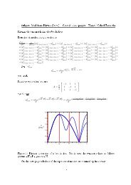
∫ r10dr 2 r 2 2 exp (−λr 2 ) = ∂2∂λ 2 ∫ r10(dr 2 exp (−λr 2 ) = ∂2∂λ 2 − exp (−λr 1)+ 1 )= ∂(λ λ ∂λ exp (−λr r11)λ + 1 )+ 2 λ 2 λ 3( (r1= exp (−λr 1 ) −r 1λ + 1 )λ 2 − r 1λ 2 − 2 )λ 3 + 2 λ 3 = − exp (−λr 1) r2 1λ 2 + 2r 1 λ + 2λ 3 + 2 λ 3∫ ∞r 1dr 2 r 2 exp (−λr 2 ) = − ∂∂λ∫ ∞r 1dr 2 exp (−λr 2 ) = − ∂∂λ( )exp (−λr1 )λ(r1= exp (−λr 1 )λ + 1 )λ 2〈ψ|Ĥ2|ψ〉 = 2ma 7 0+ 2ma 7 0= 2ma 7 0(4π) 2 ∫ ∞0(4π) 2 ∫ ∞0(4π) 2 ∫ ∞0⎛((⎜dr 1 ⎝− exp − 2α ) r2 2α1r 1a 0⎛(⎜dr 1 ⎝r 1 exp − 2α⎛⎜dr 1 ⎝− r 1 2α(= 2 a0) 3∫ ∞2 (4π)ma 7 0 2α0a 0+ 2() 32αa 0dr 1(−With equations 16 and 17 this leads to:⎛ ⎛(〈ψ|Ĥ2|ψ〉 = 2 a0) 32 ⎜ ⎜(4π)ma 7 ⎝− ⎝ 2 2α( )0 2α3+ 24α a 0a 0(= 2 a0) 52 (4π)(− 2 ma 7 0 2α8 − 2 )4 + 2So finally we solved the integral:) 2⎞a 0+2α 2r1a 0+ 2( ) 3+ (2) 32α2αa 0 a 0) ⎛ ⎞⎞⎜ r 1r 1 ⎝a2α+ 1 ⎟⎟( ) 2 ⎠⎠ r 1 exp0 a 02αa 0(exp − 4α )r 1a 0+ (2() 3exp2αa 0(⎟⎠ r 1 exp −2α r 1(−2α r 1a 0)−2α r 1a 0) ⎞ ⎟ ⎠ r1( ) (r12 2α+ 2r 1 exp − 4α )r 1 + 2r 1 expa 0 a 0⎞1 ⎟) 2 ⎠ + 2a 0(4α⎞1 ⎟) 2 ⎠a 0(2α(− 2αa 0r 1))a 0)〈ψ|Ĥ2|ψ〉 =2ma 2 0π 2 5α 5 8(35)4 Optimizing the EnergyNow we calculated all terms to get the energy (see equation 4):E (α) = 〈ψ|Ĥ|ψ〉〈ψ|ψ〉= 〈ψ|Ĥ1|ψ〉 + 〈ψ|Ĥ2|ψ〉〈ψ|ψ〉With equation 18, 20 and 35 we get the result:E (α) = − 2 π 2 (4−α)ma 2 0 α 5π 2α 6+ 2 π 2 5ma 2 0 α 5 8( )E (α) = − 2 27ma 2 0 8 α − α2(36)10

As already explained in equation 5 the first derivative of the energy must be zerodE (α)dα = 0 = d ( ))(− 2 27dα8 α − α20 = − 2ma 2 00 = 27 8 − 2αSo the optimized value for α is:ma 2 0( 278 − 2α )α = 2716(37)As we can easily see from the energy E (α) this is the global minimum. The corresponding energy is (withequation 36):( ) 27E opt = E16( ( ) ) 2= − 2 27 27 27ma 2 0 8 16 − 16(= − 2 729ma 2 0 128 − 729 )256E opt = − 2 729ma 2 0 256(38)(39)The hartree E h is the atomic unit of energy (see also equation 8):E h =2ma 2 0= e24πɛ 0 a 0(40)So in hartree the energy would beE opt = − 729 hartree256(41)= −2.8477hartree (42)Putting the values = 1.054571628 · 10 −34 Js (43)m = 9.10938215 · 10 −31 kg (44)a 0 = 5.291772186 · 10 −11 m (45)e = −1.602176487 · 10 −19 C (46)into equation 39 results in:E opt = −1.24151 · 10 −17 J (47)= −77.4887eV (48)11