Analysing genome-wide SNP data using adegenet 1.3-5

Analysing genome-wide SNP data using adegenet
1.3-5
Thibaut Jombart
November 1, 2012
Abstract
Genome-wide SNP data can quickly be challenging to analyse using
standard computer. The package adegenet [1] for the R software [2]
implements representation of these data with unprecedented efficiency
using the classes SNPbin and genlight, which can require up to 60 times
less RAM than usual representation using allele frequencies. This vignette
introduces these classes and illustrates how these objects can be handled
and analyzed in R.
1

Contents
1 Introduction 3
2 Classes of objects 3
2.1 SNPbin: storage of single genomes . . . . . . . . . . . . . . . . . 3
2.2 genlight: storage of multiple genomes . . . . . . . . . . . . . . . 6
3 Data handling using genlight objects 8
3.1 Using accessors . . . . . . . . . . . . . . . . . . . . . . . . . . . . 8
3.2 Subsetting the data . . . . . . . . . . . . . . . . . . . . . . . . . . 11
3.3 Data conversions . . . . . . . . . . . . . . . . . . . . . . . . . . . 13
3.3.1 The .snp format . . . . . . . . . . . . . . . . . . . . . . . 13
3.3.2 Importing data from PLINK . . . . . . . . . . . . . . . . 16
3.3.3 Extracting SNPs from alignments . . . . . . . . . . . . . . 16
4 Data analysis using genlight objects 19
4.1 Basic analyses . . . . . . . . . . . . . . . . . . . . . . . . . . . . . 20
4.1.1 Plotting genlight objects . . . . . . . . . . . . . . . . . . 20
4.1.2 genlight-optimized routines . . . . . . . . . . . . . . . . 22
4.1.3 Analysing data per block . . . . . . . . . . . . . . . . . . 25
4.1.4 What is the unit of observation? . . . . . . . . . . . . . . 27
4.2 Principal Component Analysis (PCA) . . . . . . . . . . . . . . . 29
4.3 Discriminant Analysis of Principal Components (DAPC) . . . . . 33
2

1 Introduction
Modern sequencing technologies now make complete genomes more widely
accessible. The subsequent amounts of genetic data pose challenges in terms
of storing and handling the data, making former tools developed for classical
genetic markers such as microsatellite impracticable using standard computers.
Adegenet has developed new object classes dedicated to handling genomewide
polymorphism (SNPs) with minimum random access memory (RAM)
requirements.
Two new formal classes have been implemented: SNPbin, used to store
genome-wide SNPs for one individual, and genlight, which stored the same
informationformultipleindividuals. Informationrepresentedthiswayisbinary:
only biallelic SNPs can be stored and analyzed using these classes. However,
these objects are otherwise very flexible, and can incorporate different levels of
ploidy across individuals within a single dataset. In this vignette, we present
these object classes and show how their content can be further handled and
content analyzed.
2 Classes of objects
2.1 SNPbin: storage of single genomes
The class SNPbin is the core representation of biallelic SNPs which allows to
represent data with unprecedented efficiency. The essential idea is to code
binary SNPs not as integers, but as bits. This operation is tricky in R as there
is no handling of bits, only bytes – series of 8 bits. However, the class SNPbin
handles this transparently using sub-rountines in C language. Considerable
efforts have been made so that the user does not have to dig into the complex
internal structure of the objects, and can handle SNPbin objects as easily as
possible.
Likegenindandgenpopobjects,SNPbinisaformal”S4”class. Thestructure
of these objects is detailed in the dedicated manpage (?SNPbin). As all S4
objects, instances of the class SNPbin are composed of slots accessible using the
@ operator. This content is generic (it is the same for all instances of the class),
and returned by:
> library(adegenet)
> getClassDef("SNPbin")
Class "SNPbin" [package "adegenet"]
Slots:
Name: snp n.loc NA.posi label ploidy
Class: list integer integer charOrNULL integer
The slots respectively contain:
3

• snp: SNP data with specific internal coding.
• n.loc: the number of SNPs stored in the object.
• NA.posi: position of the missing data (NAs).
• label: an optional label for the individual.
• ploidy: the ploidy level of the genome.
New objects are created using new, with these slots as arguments. If no
argument is provided, an empty object is created:
> new("SNPbin")
=== S4 class SNPbin ===
0 SNPs coded as bits
Ploidy: 1
0 (NaN %) missing data
In practice, only thesnp information and possibly the ploidy has to be provided;
various formats are accepted for the snp component, but the simplest is a vector
of integers (or numeric) indicating the number of second allele at each locus.
The argument snp, if provided alone, does not have to be named:
> x x
=== S4 class SNPbin ===
7 SNPs coded as bits
Ploidy: 2
0 (0 %) missing data
If not provided, the ploidy is detected from the data and determined as the
largest number in the input vector. Obviously, in many cases this will not be
adequate, but ploidy can always be rectified afterwards; for instance:
> x
=== S4 class SNPbin ===
7 SNPs coded as bits
Ploidy: 2
0 (0 %) missing data
> ploidy(x) x
=== S4 class SNPbin ===
7 SNPs coded as bits
Ploidy: 3
0 (0 %) missing data
The internal coding of the objects is cryptic, and not meant to be accessed
directly:
> x@snp
4

[[1]]
[1] 08
[[2]]
[1] 4e
Fortunately, data are easily converted back into integers:
> as.integer(x)
[1] 0 1 1 2 0 0 1
˜
The main interest of this representation is its efficiency in terms of storage.
For instance:
> dat print(object.size(dat),unit="auto")
[1] 4000040
> x print(object.size(x),unit="auto")
[1] 126320
here, we converted a million SNPs into a SNPbin object, which turns out to be
32 smaller than the original data. However, the information in dat and x is
strictly identical:
> identical(as.integer(x),dat)
[1] FALSE
The advantage of this storage is therefore being extremely compact, and
allowing to analyse big datasets using standard computers.
While SNPbin objects are the very mean by which we store data efficiently,
in practice we need to analyze several genomes at a time. This is made possible
by the class genlight, which relies on SNPbin but allows for storing data from
several genomes at a time.
5

2.2 genlight: storage of multiple genomes
Like SNPbin, genlight is a formal S4 class. The slots of instances of this class
are described by:
> getClassDef("genlight")
Class "genlight" [package "adegenet"]
Slots:
Name: gen n.loc ind.names loc.names loc.all
Class: list integer charOrNULL charOrNULL charOrNULL
Name: chromosome position ploidy pop other
Class: factorOrNULL intOrNULL intOrNULL factorOrNULL list
As it can be seen, these objects allow for storing more information in addition
to vectors of SNP frequencies. More precisely, their content is (see ?genlight
for more details):
• gen: SNP data for different individuals, each stored as a SNPbin; loci have
to be identical across all individuals.
• n.loc: the number of SNPs stored in the object.
• ind.names: (optional) labels for the individuals.
• loc.names: (optional) labels for the loci.
• loc.all: (optional) alleles of the loci separated by ’/’ (e.g. ’a/t’, ’g/c’,
etc.).
• chromosome: (optional) a factor indicating the chromosome to which the
SNPs belong.
• position: (optional) the position of each SNPs in their chromosome.
• ploidy: (optional) the ploidy of each individual.
• pop: (optional) a factor grouping individuals into ’populations’.
• other: (optional) a list containing any supplementary information to be
stored with the data.
Like SNPbin object, genlight object are created using the constructor new,
providing content for the slots above as arguments. When none is provided, an
empty object is created:
> new("genlight")
=== S4 class genlight ===
0 genotypes, 0 binary SNPs
The most important information to provide is obviously the genotypes
(argument gen); these can be provided as:
6

• a list of integer vectors representing the number of second allele at each
locus.
• a matrix / data.frame of integers, with individuals in rows and SNPs in
columns.
• a list of SNPbin objects.
Ploidy has to be consistent across loci for a given individual, but individuals
donothavetohavethesameploidy, sothatitispossibletohavehapoid, diploid,
and tetraploid individuals in the same dataset; for instance:
> x x
=== S4 class genlight ===
3 genotypes, 6 binary SNPs
Ploidy statistics (min/median/max): 1 / 2 / 4
0 (0 %) missing data
> ploidy(x)
indiv1 indiv2 toto
1 2 4
As for SNPbin, genlight objects can be converted back to integers vectors,
stored as matrices or lists:
> as.list(x)
$indiv1
[1] 1 1 0 1 1 0
$indiv2
[1] 2 1 1 0 0 0
$toto
[1] 2 2 0 0 4 4
> as.matrix(x)
[,1] [,2] [,3] [,4] [,5] [,6]
indiv1 1 1 0 1 1 0
indiv2 2 1 1 0 0 0
toto 2 2 0 0 4 4
In practice, genlight objects can be handled as if they were matrices of integers
as the one above returned by as.matrix. However, they offer the advantage of
efficient storage of the information; for instance, we can simulate 50 individuals
typed for 100,000 SNPs each (including occasional NAs):
> dat names(dat) print(object.size(dat),unit="auto")
7

[1] 40005720
> x print(object.size(x),unit="auto")
[1] 716528
> object.size(dat)/object.size(x)
55.8327378692808 bytes
here again, the storage if the data is much more efficient in genlight than
using integers: converted data occupy 56 times less memory than the original
data.
The advantage of this storage is therefore being extremely compact, and
allowing to analyse very large datasets using standard computers. Obviously,
usual computations demand data to be at one moment coded as numeric values
(as opposed to bits). However, most usual computations can be achieved
by only converting one or two genomes back to numeric values at a time,
therefore keeping RAM requirements low, albeit at a possible cost of increased
computational time. This however is minimized by three ways:
1. conversion routines are optimized for speed using C code.
2. using parallel computation where multicore architectures are available.
3. handling smaller objects, thereby decreasing the possibly high
computational time taken by memory allocation.
While this makes implementing methods more complicated. In practice,
routines are implemented so as to minimize the amount of data converted
back to integers, use C code where possible, and use multiple cores if the
package multicore is installed an multiple cores are available. Fortunately, these
underlying technical issues are oblivious to the user, and one merely needs to
know how to manipulate genlight objects using a few key functions to be able
to analyze data.
3 Data handling using genlight objects
3.1 Using accessors
In the following, we demonstrate how to manipulate and analyse genlight
objects. The phylosophy underlying formal (S4) classes in general, and
genlightobjectsinparticular, isthatinternalrepresentationoftheinformation
8

can be complex as long as accessing this information is simple. This is made
possible by decoupling storage and accession: the user is not meant to access
the content of the object directly, but has to use accessors to retrieve or
modify information.
Available accessors are documented in ?genlight. Most of them are
identical to accessors for genind and genpop objects, such as:
• nInd: returns the number of individuals in the object.
• nLoc: returns the number of loci (SNPs).
• indNames † : returns/sets labels for individuals.
• locNames † : returns/sets labels for loci (SNPs).
• alleles † : returns/sets alleles.
• ploidy † : returns/sets ploidy of the individuals.
• pop † : returns/sets a factor grouping individuals.
• other † : returns/sets misc information stored as a list.
where † indicates that a replacement method is available using dat dat
[[1]]
[1] 1 1 0 2 0 0 1 0 2 2
[[2]]
[1] 1 0 1 0 0 2 1 0 0 0
[[3]]
[1] 1 1 1 0 1 2 2 2 0 1
> x x
=== S4 class genlight ===
3 genotypes, 10 binary SNPs
Ploidy: 2
0 (0 %) missing data
> indNames(x)
NULL
> indNames(x) indNames(x)
[1] "individual 1" "individual 2" "individual 3"
9

locNames(x)
> locNames(x) as.matrix(x)
SNP.1 SNP.2 SNP.3 SNP.4 SNP.5 SNP.6 SNP.7 SNP.8 SNP.9 SNP.10
individual 1 1 1 0 2 0 0 1 0 2 2
individual 2 1 0 1 0 0 2 1 0 0 0
individual 3 1 1 1 0 1 2 2 2 0 1
In addition, some specific accessors are available for genlight objects:
• NA.posi: returns the position of missing values in each individual.
• chromosome † : returns/sets the chromosome of each SNP.
• chr † : same as chromosome — used as a shortcut.
• position † : returns/sets the position of each SNP.
Accessors are meant to be clever about replacement, meaning that they try
hard to prevent replacement with inconsistent values. For instance, in object x:
> x
=== S4 class genlight ===
3 genotypes, 10 binary SNPs
Ploidy: 2
0 (0 %) missing data
@loc.names: labels of the SNPs
if we try to set information about the chromosomes of the SNPs, the instruction:
> chr(x) chr(x) x
=== S4 class genlight ===
3 genotypes, 10 binary SNPs
Ploidy: 2
0 (0 %) missing data
@chromosome: chromosome of the SNPs
@loc.names: labels of the SNPs
> chr(x)
[1] chr-1 chr-1 chr-1 chr-1 chr-1 chr-1 chr-1 chr-1 chr-1 chr-1
Levels: chr-1
is a valid replacement.
10

3.2 Subsetting the data
genlight objects are meant to be handled as if they were matrices of allele
numbers, as returned by as.matrix. Therefore, subsetting can be achieved
using [ idx.row , idx.col ] where idx.row and idx.col are indices for rows
(individuals) and columns (SNPs). For instance, using the previous toy dataset,
we try a few classical subsetting of rows and columns:
> x
=== S4 class genlight ===
3 genotypes, 10 binary SNPs
Ploidy: 2
0 (0 %) missing data
@chromosome: chromosome of the SNPs
@loc.names: labels of the SNPs
> as.matrix(x)
SNP.1 SNP.2 SNP.3 SNP.4 SNP.5 SNP.6 SNP.7 SNP.8 SNP.9 SNP.10
individual 1 1 1 0 2 0 0 1 0 2 2
individual 2 1 0 1 0 0 2 1 0 0 0
individual 3 1 1 1 0 1 2 2 2 0 1
> as.matrix(x[c(1,3),])
SNP.1 SNP.2 SNP.3 SNP.4 SNP.5 SNP.6 SNP.7 SNP.8 SNP.9 SNP.10
individual 1 1 1 0 2 0 0 1 0 2 2
individual 3 1 1 1 0 1 2 2 2 0 1
> as.matrix(x[, c(TRUE,FALSE)])
SNP.1 SNP.3 SNP.5 SNP.7 SNP.9
individual 1 1 0 0 1 2
individual 2 1 1 0 1 0
individual 3 1 1 1 2 0
> as.matrix(x[1:2, c(1,1,1,2,2,2,3,3,3)])
SNP.1 SNP.1 SNP.1 SNP.2 SNP.2 SNP.2 SNP.3 SNP.3 SNP.3
individual 1 1 1 1 1 1 1 0 0 0
individual 2 1 1 1 0 0 0 1 1 1
Moreover, one can split data into blocks of SNPs using seploc. This can be
achieved by specifying either a number of blocks (argument n.block) or the size
of the blocks (argument block.size). The function also allows for randomizing
the distribution of the SNPs in the blocks (argument random=TRUE), which
is especially useful to replace computations that cannot be achieved on the
whole dataset with parallelized computations performed on random blocks (for
parallelization, remove the argument multicore=FALSE). For instance:
> x
11

=== S4 class genlight ===
3 genotypes, 10 binary SNPs
Ploidy: 2
0 (0 %) missing data
@chromosome: chromosome of the SNPs
@loc.names: labels of the SNPs
> as.matrix(x)
SNP.1 SNP.2 SNP.3 SNP.4 SNP.5 SNP.6 SNP.7 SNP.8 SNP.9 SNP.10
individual 1 1 1 0 2 0 0 1 0 2 2
individual 2 1 0 1 0 0 2 1 0 0 0
individual 3 1 1 1 0 1 2 2 2 0 1
> seploc(x, n.block=2, multicore=FALSE)
$block.1
=== S4 class genlight ===
3 genotypes, 5 binary SNPs
Ploidy: 2
0 (0 %) missing data
@chromosome: chromosome of the SNPs
@loc.names: labels of the SNPs
$block.2
=== S4 class genlight ===
3 genotypes, 5 binary SNPs
Ploidy: 2
0 (0 %) missing data
@chromosome: chromosome of the SNPs
@loc.names: labels of the SNPs
> lapply(seploc(x, n.block=2, multicore=FALSE),as.matrix)
$block.1
SNP.1 SNP.2 SNP.3 SNP.4 SNP.5
individual 1 1 1 0 2 0
individual 2 1 0 1 0 0
individual 3 1 1 1 0 1
$block.2
SNP.6 SNP.7 SNP.8 SNP.9 SNP.10
individual 1 0 1 0 2 2
individual 2 2 1 0 0 0
individual 3 2 2 2 0 1
splits the data into two blocks of contiguous SNPs, while:
> lapply(seploc(x, n.block=2, random=TRUE, multicore=FALSE),as.matrix)
$block.1
SNP.1 SNP.3 SNP.7 SNP.2 SNP.10
individual 1 1 0 1 1 2
individual 2 1 1 1 0 0
individual 3 1 1 2 1 1
$block.2
SNP.9 SNP.4 SNP.6 SNP.8 SNP.5
individual 1 2 2 0 0 0
individual 2 0 0 2 0 0
individual 3 0 0 2 2 1
generates blocks of randomly selected SNPs.
12

3.3 Data conversions
3.3.1 The .snp format
adegenet has defined its own format for storing biallelic SNP data in text files
with extension .snp. This format has several advantages: it is fairly compact
(more so than usual non-compressed formats), allows for any information about
individuals or loci to be stored, allows for comments, and is easily parsed — in
particular, not all information has to be read at a time, again minimizing RAM
requirements for import procedures.
Anexamplefileofthisformatisdistributedwithadegenet. Oncethepackage
has been installed, the file can be accessed by typing:
> file.show(system.file("files/exampleSnpDat.snp",package="adegenet"))
Otherwise, this file is also accessible from the adegenet website (section
’Documents’). A complete description of the .snp format is provided in the
comment section of the file.
The structure of a .snp file can be summarized as follows:
• a (possibly empty) comment section
• meta-information, i.e. information about loci or individuals, stored as
named vectors
• genotypes, stored as named vectors
The comment section can starts with the line:
>>>> begin comments - do not remove this line > end comments - do not remove this line

• population: character strings indicating a group memberships of the
individuals
• ploidy: integers indicating the ploidy of each individual; alternatively,
one single integer if all individuals have the same ploidy
• chromosome: character strings indicating the chromosome on which the
SNP are located
Each genotype is stored using two lines, the first being:
> label-of-the-individual
and the second being integers corresponding to the number of second allele for
each loci, without separators; missing data are coded as ’-’.
.snp files can be read in R using read.snp, which converts data into
genlight objects. The function reads data by chunks of a several individuals
(minimum 1, no maximum besides RAM constraints) at a time, which allows
one to read massive datasets with negligible RAM requirements (albeit at a
cost of computational time). The argument chunkSize indicates the number of
genomes read at a time; larger values mean reading data faster but require more
RAM. We can illustrate read.snp using the example file mentioned above. The
non-comment part of the file reads:
[...]
>> position
1 8 11 43
>> allele
a/t g/c a/c t/a
>> population
Brit Brit Fren monster NA
>> ploidy
2
> foo
1020
> bar
0012
> toto
10-0
> Nyarlathotep
0120
> an even longer label but OK since on a single line
1100
We read the file in using:
> obj

Reading biallelic SNP data file into a genlight object...
Reading comments...
Reading general information...
Reading 5 genotypes...
...
Checking consistency...
Building final object...
...done.
> obj
=== S4 class genlight ===
5 genotypes, 4 binary SNPs
Ploidy: 2
1 (0.05 %) missing data
@pop: individual membership for 4 populations
@position: position of the SNPs
@alleles: alleles of the SNPs
> as.matrix(obj, multicore=FALSE)
1.a/t 8.g/c 11.a/c 43.t/a
foo 1 0 2 0
bar 0 0 1 2
toto 1 0 NA 0
Nyarlathotep 0 1 2 0
an even longer label but OK since on a single line 1 1 0 0
> alleles(obj)
[1] "a/t" "g/c" "a/c" "t/a"
> pop(obj)
[1] Brit Brit Fren monster NA
Levels: Brit Fren NA monster
> indNames(obj)
[1] "foo"
[2] "bar"
[3] "toto"
[4] "Nyarlathotep"
[5] "an even longer label but OK since on a single line"
Note that system.file is generally useless: it is only used in this example
to access a file installed alongside the package. Usual calls to read.snp will
ressemble:
> obj

3.3.2 Importing data from PLINK
Genome-wide SNP data of diploid organisms are frequently analyzed
using PLINK, whose format is therefore becoming a standard. Data
with PLINK format (.raw) can be imported into genlight objects
using read.PLINK. This function requires the data to be saved in
PLINK using the ‘-recodeA‘ option (see details section in ?read.PLINK).
More information on exporting from PLINK can be found at http:
//pngu.mgh.harvard.edu/~purcell/plink/dataman.shtml#recode.
Like read.snp, read.PLINK has the advantage of reading data by chunks
of a few individuals (down to a single one at a time, no upper limits),
which minimizes the amount of memory needed to read information before
its conversion to genlight; however, using more chunks also means more
computational time, since the procedure has to re-read the same file several
time. Note that meta information about the loci also known as .map can also
be read alongside a .raw file using the argument map.file. Alternatively,
such information can be added to a genlight object afterwards using
extract.PLINKmap.
3.3.3 Extracting SNPs from alignments
In many cases, raw genomic data are available as aligned sequences, in which
case extracting polymorphic sites can be non-trivial. The biggest issue is again
memory: most software extracting SNPs from aligned sequences require all
the sequences to be stored in memory at a time, a duty that most common
computers cannot undertake. adegenet implements a more parsimonious
alternative which allows for extracting SNPs from alignment while processing
a reduced number of sequences (down to a single) at a time.
The function fasta2genlight extracts SNPs from alignments with fasta
format (file extensions ’.fasta’, ’.fas’, or ’.fa’). Like read.snp and
read.PLINK, fasta2genlight processes data by chunks of individuals so as
to save memory requirements. It first scans the whole file for polymorphic
positions, and then extracts all biallelic SNPs from the alignment.
fasta2genlight is illustrated like read.snp using a toy dataset distributed
alongside the package. The file is first located using system.file, and then
processed using fasta2genlight:
> myPath flu

Building final object...
...done.
> flu
=== S4 class genlight ===
80 genotypes, 274 binary SNPs
Ploidy: 1
26 (0 %) missing data
@position: position of the SNPs
@alleles: alleles of the SNPs
flu is a genlight object containing SNPs of 80 isolates of seasonal influenza
(H3N2) sampled within the US over the last two decades; sequences correspond
to the hemagglutinin (HA) segment. Besides genotypes, flu contains the
positions of the SNPs and the alleles at each retained loci. Names of the loci
are constructed as the combination of both:
> head(position(flu), 20)
[1] 7 12 31 32 36 37 44 45 52 60 62 72 73 78 96 99 105 108 121
[20] 128
> head(alleles(flu), 20)
[1] "a/g" "c/t" "t/c" "t/c" "t/c" "c/a" "t/c" "c/t" "a/g" "c/t" "g/t" "c/a"
[13] "a/g" "a/g" "a/g" "c/t" "a/g" "g/a" "c/a" "a/g"
> head(locNames(flu), 20)
[1] "7.a/g" "12.c/t" "31.t/c" "32.t/c" "36.t/c" "37.c/a" "44.t/c"
[8] "45.c/t" "52.a/g" "60.c/t" "62.g/t" "72.c/a" "73.a/g" "78.a/g"
[15] "96.a/g" "99.c/t" "105.a/g" "108.g/a" "121.c/a" "128.a/g"
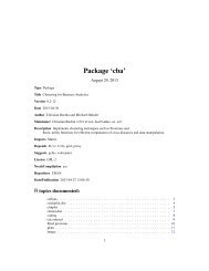
It is usually informative to assess the position of the polymorphic sites within
the genome; this is very easily done in R, using density with an appropriate
bandewidth:
> temp plot(temp, type="n", xlab="Position in the alignment", main="Location of the SNPs",
+ xlim=c(0,1701))
> polygon(c(temp$x,rev(temp$x)), c(temp$y, rep(0,length(temp$x))), col=transp("blue",.3))
> points(position(flu), rep(0, nLoc(flu)), pch="|", col="blue")
17

Density
0.0000 0.0005 0.0010 0.0015
Location of the SNPs
| ||||| ||||| |||||||| | || | || |||||| || ||| | |||| |||||||||| || ||||| | ||||||| ||| |||||||| |||| |||| ||
0 500 1000 1500
Position in the alignment
In this case, SNPs are distributed fairly homogeneously across the HA segment,
with a few possible hotspots of polymorphism within positions 400—700.
Note that retaining only biallelic sites may cause minor loss of information,
as sites with more than 2 alleles are discarded from the data. It is however
possible to ask fasta2genlight to keep track of the number of alleles for each
site of the original alignment, by specifying:
> flu flu
=== S4 class genlight ===
80 genotypes, 274 binary SNPs
Ploidy: 1
26 (0 %) missing data
@position: position of the SNPs
@alleles: alleles of the SNPs
@other: a list containing: nb.all.per.loc
The output object flu now contains the number of alleles of each position,
stored in the other slot:
> head(other(flu)$nb.all.per.loc, 20)
[1] 1 1 1 1 1 1 2 1 1 1 1 2 1 1 1 1 1 1 1 1
> 100*mean(unlist(other(flu))>1)
18

[1] 17.81305
About 18% of the sites are polymorphic, which is fairly high. This is not entirely
surprising, giventhattheHAsegmentofinfluenzaisknownforitshighmutation
rate. What is the nature of this polymorphism?
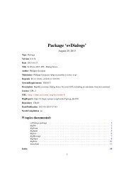
> temp barplot(temp, main="Distribution of the number \nof alleles per loci",
+ xlab="Number of alleles", ylab="Number of sites", col=heat.colors(4))
Number of sites
0 200 400 600 800 1000 1200
Distribution of the number
of alleles per loci
1 2 3 4
Number of alleles
Most polymorphic loci are biallelic, but a few loci with 3 or 4 alleles were lost.
We can estimate the loss of information very simply:
> temp temp round(temp,1)
2 3 4
90.4 8.3 1.3
In this case, 90.4% of the polymorphic sites were biallelic, the others being
essentially triallelic. This is probably a fairly exceptional situation due to the
high mutation rate of the HA segment.
4 Data analysis using genlight objects
In the following, we illustrate some methods for the analysis of genlight
objects, ranging from simple tools for diagnosing allele frequencies or missing
19

data to recently developed multivariate approaches. Some examples below
are illustrated using toy datasets generated using the function glSim. This
simple simulation tool allows for simulating large SNPs data with possibly
contrasted structures between two groups of individuals or patterns of linkage
disequilibrium (LD). See ?glSim for more details on this tool.
4.1 Basic analyses
4.1.1 Plotting genlight objects
Basic features of the data may also be inferred by simply looking at the data.
genlight objects can be plotted using glPlot, or simply plot (both names
actually correspond to the same function). This function displays the data as
images, representing numbers of second alleles using colours. For instance, we
can have a feel for the amount and location of missing data in the influenza
dataset (see previous section) fairly easily:
> glPlot(flu, posi="topleft")
The white streches in the first 30 SNPs observed around individual 70 indicate
missing data. There are only a few missing data, and they only concern a
couple of individuals.
In some simple cases, some biological structures might also be apparent
in such plot. For instance, we can generate data with independent SNPs
distributions for two groups:
> x plot(x)
20

Strong patterns of LD between contiguous sites are also very easy to spot:
> x plot(x)
21

Of course, this is merely a very preliminary approach to the data. More
detailed analysis can be achieved using both standard and ad hoc procedures as
detailed below.
4.1.2 genlight-optimized routines
Some simple operations such as computing allele frequencies or diagnosing
missing values can be problematic when the data matrix cannot be represented
in memory. adegenet implements a few basic procedures which perform such
basic tasks on genlight objects processing one individual at a time, thereby
minimizing memory requirements. The most computer-intensive of these
procedures can also use compiled C code and/or multicore capabilities (when
available) to speed up computations.
All these procedures are named using the prefix gl (for genlight), and can
therefore be listed by typing gl and pressing the TAB key twice. They are (see
?glMean):
• glSum: computes the sum of second alleles for each SNP.
• glNA: computes the number of missing values in each locus.
• glMean: computes the mean of second alleles, i.e. second allele frequencies
for each SNP.
22

• glVar: computes the variance of the second allele frequency for each SNP.
• glDotProd: computes the dot products between all pairs of individuals,
with possible centring and scaling.
For instance, one can easily derive the distributiong of allele frequencies using:
> myFreq hist(myFreq, proba=TRUE, col="gold", xlab="Allele frequencies",
+ main="Distribution of (second) allele frequencies")
> temp lines(temp$x, temp$y*1.8,lwd=3)
Density
0 1 2 3 4 5 6
Distribution of (second) allele frequencies
0.0 0.2 0.4 0.6 0.8 1.0
Allele frequencies
In biallelic loci, one allele is always entirely redundant with the other, so it is
generally sufficient to analyse a single allele per loci. However, the distribution
of allele frequencies may be more interpretable by restoring its native symmetry:
> myFreq myFreq hist(myFreq, proba=TRUE, col="darkseagreen3", xlab="Allele frequencies",
+ main="Distribution of allele frequencies", nclass=20)
> temp lines(temp$x, temp$y*2,lwd=3)
23

Density
0 1 2 3 4 5
Distribution of allele frequencies
0.0 0.2 0.4 0.6 0.8 1.0
Allele frequencies
While a large number of loci are nearly fixed (frequencies close to 0 or 1),
there is an appreciable number of alleles with intermediate frequencies and
therefore susceptible to contain interesting biological signal. More generally
and perhaps more importantly, this figure may also cast light on a well-known
social phenomenon occuring mainly in young people attending noisy kinds of
conferences:
We can indeed wonder whether the gesture usually referred to as the ’devil sign’
is not actually a reference to the usual shape of SNPs frequency distributions.
24

It is still unclear, however, how many geneticists do attend metal gigs, although
recent observations suggest they would be more frequent in grindcore events
than in classical heavy metal shows.
Besides these considerations, we can also map missing data across loci as we
have done for SNP positions in the US influenza dataset (see previous section)
using glNA and density:
> head(glNA(flu),20)
7.a/g 12.c/t 31.t/c 32.t/c 36.t/c 37.c/a 44.t/c 45.c/t 52.a/g 60.c/t
2 2 2 2 2 2 2 2 1 1
62.g/t 72.c/a 73.a/g 78.a/g 96.a/g 99.c/t 105.a/g 108.g/a 121.c/a 128.a/g
1 1 1 1 1 1 0 0 0 0
> temp plot(temp, type="n", xlab="Position in the alignment", main="Location of the missing values (NAs)",
+ xlim=c(0,1701))
> polygon(c(temp$x,rev(temp$x)), c(temp$y, rep(0,length(temp$x))), col=transp("blue",.3))
> points(glNA(flu), rep(0, nLoc(flu)), pch="|", col="blue")
Here, the few missing values are all located at the beginning at the alignment,
probably reflecting heterogeneity in DNA amplification during the sequencing
process. In larger datasets, such simple investigation can give crucial insights
about the quality of the data and the existence of possible sequencing biases.
4.1.3 Analysing data per block
Some operations such as computations of distances between individuals can
also be useful, and have yet to be implemented for genlight objects. These
operations are easy to carry out by converting data to alleles counts (using
as.matrix), but this conversion itself can be problematic because of memory
limitations. One easy workaround consists in parallelizing computations across
blocks of loci. seploc is first used to create a list of smaller genlight objects,
each of which can individually be converted to absolute allele frequencies using
as.matrix. Then, computations are carried on the list of object, without ever
having to convert the entire dataset, and results are finally reunited.
Let us illustrate this procedure using 40 simulated individuals with 10,000
SNPs each:
> x x
=== S4 class genlight ===
40 genotypes, 10000 binary SNPs
Ploidy: 1
0 (0 %) missing data
@pop: individual membership for 2 populations
seploc is used to create a list of smaller objects (here, 10 blocks of 10,000
SNPs):
25

x class(x)
[1] "list"
> names(x)
[1] "block.1" "block.2" "block.3" "block.4" "block.5" "block.6"
[7] "block.7" "block.8" "block.9" "block.10"
> x[1:2]
$block.1
=== S4 class genlight ===
40 genotypes, 1000 binary SNPs
Ploidy: 1
0 (0 %) missing data
@pop: individual membership for 2 populations
$block.2
=== S4 class genlight ===
40 genotypes, 1000 binary SNPs
Ploidy: 1
0 (0 %) missing data
@pop: individual membership for 2 populations
dist is used within a lapply loop to compute pairwise distances between
individuals for each block:
> lD class(lD)
[1] "list"
> names(lD)
[1] "block.1" "block.2" "block.3" "block.4" "block.5" "block.6"
[7] "block.7" "block.8" "block.9" "block.10"
> class(lD[[1]])
[1] "dist"
lD is a list of distances matrices (dist objects) between pairs of individuals.
The general distance matrix is obtained by summing these:
> D library(ape)
> plot(nj(D), type="fan")
> title("A simple NJ tree of simulated genlight data")
26

A simple NJ tree of simulated genlight data
ind 14
ind 34
ind 11
ind 24
ind 22
ind 6
ind 31
ind 5
ind 25
ind 17
ind 32
ind 12
ind 16
ind 1
ind 36
ind 20
ind 4
ind 3
ind 40
ind 10
ind 28
ind 30
ind 35
ind 8
ind 13
ind 21
ind 23
ind 18
ind 19
ind 26
ind 15
ind 38 ind 39
4.1.4 What is the unit of observation?
ind 29
ind 9
ind 2
ind 33
ind 27
ind 37
Whenever ploidy varies across individuals, an issue arises as to what is defined
as the unit of observation. Technically speaking, the unit of observation is the
entity on which the observation is made. When working with allelic data, it is
not always clear what the unit of observation is. The unit of observation may
be:
• individuals: in this case each individual is represented by a vector of allele
frequencies
• alleles: in this case we consider that each individual represents a sample
of alleles, with a sample size equalling the ploidy for each locus
This distinction is most of the time overlooked when analysing genetic data.
Asamatteroffact, itdoesnotmatterwhenallindividualshavethesameploidy.
For instance, if we take the following data:
> x locNames(x) x
=== S4 class genlight ===
3 genotypes, 4 binary SNPs
Ploidy: 1
0 (0 %) missing data
@loc.names: labels of the SNPs
27
ind 7

as.matrix(x)
1 2 3 4
a 0 0 1 1
b 1 1 0 0
c 1 1 1 1
and assume that all individuals are haploid, then computing e.g. the allele
frequencies is straightforward (they all equal 2/3):
> glMean(x)
1 2 3 4
0.6666667 0.6666667 0.6666667 0.6666667
Let us no consider a sightly different case:
> x locNames(x) x
=== S4 class genlight ===
3 genotypes, 4 binary SNPs
Ploidy statistics (min/median/max): 1 / 1 / 2
0 (0 %) missing data
@loc.names: labels of the SNPs
> as.matrix(x)
1 2 3 4
a 0 0 2 2
b 1 1 0 0
c 1 1 1 1
> ploidy(x)
a b c
2 1 1
What are the allele frequencies in this case? Well, it depends on what we mean
by ’allele frequency’.
Is it the frequency of the alleles in the population? In this case, the unit of
observation is the allele. We have a total of 4 samples for each loci, (since ’a’
is diploid, it represents actually two samples) and the frequencies are 1/2, 1/2,
3/4, 3/4. Note, however, that this assumes that alleles are randomly associated
within individuals (pangamy).
Or is it the frequency of the alleles within the individuals? In this case,
the unit of observation is the individual, and the vector of allele frequencies
represents the ’average individual’. We first need to convert each individual
vector into relative frequencies (i.e., divide by their respective ploidy), and then
compute the average frequency across individuals, which ends up with 2/3 for
each locus:
28

M apply(M,2,mean)
1 2 3 4
0.6666667 0.6666667 0.6666667 0.6666667
The procedures designed for genlight objects seen above (glMean, glNA,
etc.) allow for this distinction to be made. The option alleleAsUnit is a
logical indicating whether the observation unit is the allele (TRUE, default) or
the individual (FALSE). For instance:
> as.matrix(x)
1 2 3 4
a 0 0 2 2
b 1 1 0 0
c 1 1 1 1
> glMean(x, alleleAsUnit=TRUE)
1 2 3 4
0.50 0.50 0.75 0.75
> glMean(x, alleleAsUnit=FALSE)
1 2 3 4
0.6666667 0.6666667 0.6666667 0.6666667
4.2 Principal Component Analysis (PCA)
Principal Component Analysis (PCA) is implemented for genlight objects by
the function glPca. This function can accommodate any level of ploidy in
the data (including varying ploidy across individuals). More importantly, it
performs computations without ever processing more than a couple of genomes
at a time, thereby minimizing memory requirements. It also uses compiled C
code and possibly multicore ressources if available to speed up computations.
We illustrate the method on the previously introduced influenza dataset (object
flu):
> pca1

0 2 4 6 8 10
Eigenvalues
When nf (number of retained factors) is not specified, the function displays the
barplot of eigenvalues of the analysis and asks the user for a number of retained
principal components. glPca returns a list with the class glPca containing the
eigenvalues, principal components and loadings of the analysis:
> pca1
=== PCA of genlight object ===
Class: list of type glPca
Call ($call):glPca(x = flu)
Eigenvalues ($eig):
11.385 4.019 1.391 1.275 0.636 0.569 ...
Principal components ($scores):
matrix with 80 rows (individuals) and 4 columns (axes)
Principal axes ($loadings):
matrix with 274 rows (SNPs) and 4 columns (axes)
In addition to usual graphics, glPca object can displayed using scatter
(produces a scatterplot of the principal components (PCs)) and loadingplot
(plotstheallelecontributions,i.e. squaredloadings). Thescatterplotisobtained
by:
> scatter(pca1, posi="bottomright")
> title("PCA of the US influenza data\n axes 1-2")
30

CY010036 CY009476 CY011128
CY010748 CY012504
CY012568 CY012288 CY012272 CY011528 CY017291 CY012480 CY013781 CY013200 CY013613 CY012160 CY010988 CY013016 CY012128
CY001616
CY008964 CY006627 CY006787 CY006243 CY006259 CY006267 CY006595 CY006235 CY006563 CY001413
CY010028 CY011424
PCA of the US influenza data
axes 1−2
CY001152 CY000584 CY000185 CY000545 CY003096 CY002328 CY001720 CY000297
CY000289 CY001552
CY002816
CY003785 CY000737 CY003272 CY001453 CY000657 CY001365 CY000705 CY002384 CY001704
CY000105
CY002104
CY000353
CY001648
d = 2
CY002432 CY019301 CY019285 CY019245 CY021989 CY003664 CY006155 CY003336
CY003640
CY034116 CY019843 EF554795
EU100713
CY019859 CY014159
EU199369
EU199254 EU779500 EU516036 CY031555 EU779498 EU516212 EU852005 CY035190 FJ549055
Eigenvalues
The first PC suggests the existence of two clades in the data, while the second
one shows groups of closely related isolates arranged along a cline of genetic
differentiation. This structure is confirmed by a simple neighbour-joining (NJ)
tree:
> library(ape)
> tre tre
Phylogenetic tree with 80 tips and 78 internal nodes.
Tip labels:
CY013200, CY013781, CY012128, CY013613, CY012160, CY012272, ...
Unrooted; includes branch lengths.
> plot(tre, typ="fan", cex=0.7)
> title("NJ tree of the US influenza data")
The correspondance between both analyses can be better assessed using
colors based on PCs; this is achieved by colorplot:
> myCol abline(h=0,v=0, col="grey")
> add.scatter.eig(pca1$eig[1:40],2,1,2, posi="topright", inset=.05, ratio=.3)
31

PC2
−3 −2 −1 0 1 2 3
−4 −2 0 2 4
PC1
> plot(tre, typ="fan", show.tip=FALSE)
> tiplabels(pch=20, col=myCol, cex=4)
> title("NJ tree of the US influenza data")
32
Eigenvalues

NJ tree of the US influenza data
As expected, both approaches give congruent results, but both are
complementary: NJ is better at showing bunches of related isolates, but the
cline of genetic differentiation is much clearer in PCA.
4.3 Discriminant Analysis of Principal Components
(DAPC)
Discriminant analysis of Principal Components (DAPC) is implemented for
genlight objects by an appropriate method for the find.clusters and dapc
generics. To put it simply, you can run find.clusters and dapc on genlight
objects and the appropriate functions will be used. As in glPca, these methods
never require more than a couple of genomes to be translated into allele
frequencies at a time, thereby minimizing RAM requirements.
Below, we illustrate DAPC on a genlight with 100 individuals, including
only 50 structured SNPs out of 10,000 non-structured SNPs:
> x dapc1

scatter(dapc1,scree.da=FALSE, bg="white", posi.pca="topright", legend=TRUE,
+ txt.leg=paste("group", 1:2), col=c("red","blue"))
Density
0.0 0.1 0.2 0.3 0.4 0.5
| | | | | | |
| | | | | | | | | | | |
|
| | | | | |
| | | | | |
| | | | | | | | | | |
| || | | | | |
| | | |
−4 −2 0 2 4
Discriminant function 1
group 1
group 2
While the composition plot confirms that groups are not entirely disentangled...
> compoplot(dapc1, col=c("red","blue"),lab="", txt.leg=paste("group", 1:2), ncol=2)
34

membership probability
0.0 0.2 0.4 0.6 0.8 1.0
group 1 group 2
... the loading plot identifies pretty well the most discriminating alleles:
> loadingplot(dapc1$var.contr, thres=1e-3)
35

And we can zoom in to the contributions of the last 100 SNPs to make sure that
the tail indeed corresponds to the 50 last structured loci:
> loadingplot(tail(dapc1$var.contr[,1],100), thres=1e-3)
36

Here, we indeed identified the structured region of the genome fairly well.
References
[1] Jombart, T. (2008) adegenet: a R package for the multivariate analysis of
genetic markers. Bioinformatics 24: 1403-1405.
[2] R Development Core Team (2011). R: A language and environment for
statistical computing. R Foundation for Statistical Computing, Vienna,
Austria. ISBN 3-900051-07-0.
37