MATLAB Function Reference (Volume 2: Graphics)

MATLAB®The Language of Technical ComputingComputationVisualizationProgrammingMATLAB Function Reference(Volume 2: Graphics)Version 5

How to Contact The MathWorks:☎PHONEFAX✉MAIL508-647-7000 Phone508-647-7001 FaxThe MathWorks, Inc.24 Prime Park WayNatick, MA 01760-1500MailINTERNET@E-MAILhttp://www.mathworks.comftp.mathworks.comcomp.soft-sys.matlabsupport@mathworks.comsuggest@mathworks.combugs@mathworks.comdoc@mathworks.comsubscribe@mathworks.comservice@mathworks.cominfo@mathworks.comWebAnonymous FTP serverNewsgroupTechnical supportProduct enhancement suggestionsBug reportsDocumentation error reportsSubscribing user registrationOrder status, license renewals, passcodesSales, pricing, and general informationMATLAB Function Reference© COPYRIGHT 1984 - 1999 by The MathWorks, Inc.The software described in this document is furnished under a license agreement. The software may be usedor copied only under the terms of the license agreement. No part of this manual may be photocopied or reproducedin any form without prior written consent from The MathWorks, Inc.U.S. GOVERNMENT: If Licensee is acquiring the Programs on behalf of any unit or agency of the U.S.Government, the following shall apply: (a) For units of the Department of Defense: the Government shallhave only the rights specified in the license under which the commercial computer software or commercialsoftware documentation was obtained, as set forth in subparagraph (a) of the Rights in CommercialComputer Software or Commercial Software Documentation Clause at DFARS 227.7202-3, therefore therights set forth herein shall apply; and (b) For any other unit or agency: NOTICE: Notwithstanding anyother lease or license agreement that may pertain to, or accompany the delivery of, the computer softwareand accompanying documentation, the rights of the Government regarding its use, reproduction, and disclosureare as set forth in Clause 52.227-19 (c)(2) of the FAR.MATLAB, Simulink, Stateflow, Handle Graphics, and Real-Time Workshop are registered trademarks, andTarget Language Compiler is a trademark of The MathWorks, Inc.Other product or brand names are trademarks or registered trademarks of their respective holders.Printing History: December 1996 First printing (for MATLAB 5)June 1997 Revised for 5.1 (online version)October 1997 Revised for 5.2 (online version)January 1999 Revised for Release 11 (online version)

Contents1Command SummaryGeneral Purpose Commands . . . . . . . . . . . . . . . . . . . . . . . . . . . . . . . . 1-2Operators and Special Characters . . . . . . . . . . . . . . . . . . . . . . . . . . 1-3Logical Functions . . . . . . . . . . . . . . . . . . . . . . . . . . . . . . . . . . . . . . . . . . . . 1-4Language Constructs and Debugging . . . . . . . . . . . . . . . . . . . . . . . 1-4Elementary Matrices and Matrix Manipulation . . . . . . . . . . . . 1-6Specialized Matrices . . . . . . . . . . . . . . . . . . . . . . . . . . . . . . . . . . . . . . . . . 1-8Elementary Math Functions . . . . . . . . . . . . . . . . . . . . . . . . . . . . . . . . . 1-8Specialized Math Functions . . . . . . . . . . . . . . . . . . . . . . . . . . . . . . . . . 1-9Coordinate System Conversion . . . . . . . . . . . . . . . . . . . . . . . . . . . . . 1-9Matrix Functions - Numerical Linear Algebra . . . . . . . . . . . . . 1-10Data Analysis and Fourier Transform Functions . . . . . . . . . . 1-11Polynomial and Interpolation Functions . . . . . . . . . . . . . . . . . . 1-13Function Functions – Nonlinear Numerical Methods . . . . . 1-13Sparse Matrix Functions . . . . . . . . . . . . . . . . . . . . . . . . . . . . . . . . . . . 1-14Sound Processing Functions . . . . . . . . . . . . . . . . . . . . . . . . . . . . . . . 1-15Character String Functions . . . . . . . . . . . . . . . . . . . . . . . . . . . . . . . . 1-16Low-Level File I/O Functions . . . . . . . . . . . . . . . . . . . . . . . . . . . . . . . 1-17i

Bitwise Functions . . . . . . . . . . . . . . . . . . . . . . . . . . . . . . . . . . . . . . . . . . 1-18Structure Functions . . . . . . . . . . . . . . . . . . . . . . . . . . . . . . . . . . . . . . . . 1-18Object Functions . . . . . . . . . . . . . . . . . . . . . . . . . . . . . . . . . . . . . . . . . . . 1-18Cell Array Functions . . . . . . . . . . . . . . . . . . . . . . . . . . . . . . . . . . . . . . . 1-18Multidimensional Array Functions . . . . . . . . . . . . . . . . . . . . . . . . 1-19Plotting and Data Visualization . . . . . . . . . . . . . . . . . . . . . . . . . . . 1-19Graphical User Interface Creation . . . . . . . . . . . . . . . . . . . . . . . . 1-252ReferenceAList of CommandsFunction Names . . . . . . . . . . . . . . . . . . . . . . . . . . . . . . . . . . . . . . . . . . . . . A–2iiContents

1Command SummaryThis chapter lists MATLAB commands by functional area.

General Purpose CommandsManaging Commands and Functionsaddpath Add directories to MATLAB’s search pathdocDisplay HTML documentation in Web browserdocopt Display location of help file directory for UNIX platformshelpOnline help for MATLAB functions and M-fileshelpdesk Display Help Desk page in Web browser, giving access to extensive helphelpwin Display Help Window, providing access to help for all commandslasterr Last error messagelastwarn Last warning messagelookfor Keyword search through all help entriespartialpath Partial pathnamepathControl MATLAB’s directory search pathpathtool Start Path Browser, a GUI for viewing and modifying MATLAB’s pathprofile Start the M-file profiler, a utility for debugging and optimizing codeprofreport Generate a profile reportrmpath Remove directories from MATLAB’s search pathtypeList fileverDisplay version information for MATLAB, Simulink, and toolboxesversion MATLAB version numberwebPoint Web browser at file or Web sitewhatDirectory listing of M-files, MAT-files, and MEX-fileswhatsnew Display README files for MATLAB and toolboxeswhich Locate functions and filesManaging Variables and the Workspaceclear Remove items from memorydispDisplay text or arraylength Length of vectorloadRetrieve variables from diskmlock Prevent M-file clearingmunlock Allow M-file clearingopenvar Open workspace variable in Array Editor, for graphical editingpackConsolidate workspace memorysaveSave workspace variables on disksaveas Save figure or model using specified formatsizeArray dimensionswho, whos List directory of variables in memoryworkspace Display the Workspace Browser, a GUI for managing the workspace1-2

Controlling the Command WindowclcechoformathomemoreClear command windowEcho M-files during executionControl the output display formatSend the cursor homeControl paged output for the command windowWorking with Files and the Operating EnvironmentcdChange working directorycopyfile Copy filedelete Delete files and graphics objectsdiary Save session in a disk filedirDirectory listingeditEdit an M-filefileparts Filename partsfullfile Build full filename from partsinmem Functions in memorylsList directory on UNIXmatlabroot Root directory of MATLAB installationmkdir Make directoryopenOpen files based on extensionpwdDisplay current directorytempdir Return the name of the system’s temporary directorytempname Unique name for temporary file! Execute operating system commandStarting and Quitting MATLABmatlabrcquitstartupMATLAB startup M-fileTerminate MATLABMATLAB startup M-fileOperators and Special Characters+ Plus- Minus* Matrix multiplication.* Array multiplication^Matrix power.^ Array powerkronKronecker tensor product1-3

Logical Functions\ Backslash or left division/ Slash or right division./ and .\ Array division, right and left: Colon( ) Parentheses[ ] Brackets{} Curly braces. Decimal point... Continuation, Comma; Semicolon% Comment! Exclamation point'Transpose and quote.'Nonconjugated transpose= Assignment== Equality< > Relational operators&Logical AND| Logical OR~ Logical NOTxorLogical EXCLUSIVE ORallanyexistfindis*isalogicalmislockedTest to determine if all elements are nonzeroTest for any nonzerosCheck if a variable or file existsFind indices and values of nonzero elementsDetect stateDetect an object of a given classConvert numeric values to logicalTrue if M-file cannot be clearedLanguage Constructs and DebuggingMATLAB as a Programming Languagebuiltin Execute builtin function from overloaded methodevalInterpret strings containing MATLAB expressionsevalc Evaluate MATLAB expression with capture1-4

evalinfevalfunctionglobalnargchkpersistentscriptEvaluate expression in workspaceFunction evaluationFunction M-filesDefine global variablesCheck number of input argumentsDefine persistent variableScript M-filesControl Flowbreak Terminate execution of for loop or while loopcaseCase switchcatch Begin catch blockelseConditionally execute statementselseif Conditionally execute statementsendTerminate for, while, switch, try, and if statements or indicate lastindexerror Display error messagesforRepeat statements a specific number of timesifConditionally execute statementsotherwise Default part of switch statementreturn Return to the invoking functionswitch Switch among several cases based on expressiontryBegin try blockwarning Display warning messagewhile Repeat statements an indefinite number of timesInteractive Inputinput Request user inputkeyboard Invoke the keyboard in an M-filemenuGenerate a menu of choices for user inputpause Halt execution temporarilyObject-Oriented Programmingclass Create object or return class of objectdouble Convert to double precisioninferiorto Inferior class relationshipinline Construct an inline objectint8, int16, int32Convert to signed integerisaDetect an object of a given class1-5

loadobj Extends the load function for user objectssaveobj Save filter for objectssingle Convert to single precisionsuperiorto Superior class relationshipuint8, uint16, uint32Convert to unsigned integerDebuggingdbcleardbcontdbdowndbmexdbquitdbstackdbstatusdbstepdbstopdbtypedbupClear breakpointsResume executionChange local workspace contextEnable MEX-file debuggingQuit debug modeDisplay function call stackList all breakpointsExecute one or more lines from a breakpointSet breakpoints in an M-file functionList M-file with line numbersChange local workspace contextElementary Matrices and Matrix ManipulationElementary Matrices and Arraysblkdiag Construct a block diagonal matrix from input argumentseyeIdentity matrixlinspace Generate linearly spaced vectorslogspace Generate logarithmically spaced vectorsonesCreate an array of all onesrandUniformly distributed random numbers and arraysrandn Normally distributed random numbers and arrayszeros Create an array of all zeros: (colon) Regularly spaced vectorSpecial Variables and ConstantsanscomputerepsflopsiThe most recent answerIdentify the computer on which MATLAB is runningFloating-point relative accuracyCount floating-point operationsImaginary unit1-6

InfInfinityinputname Input argument namejImaginary unitNaNNot-a-Numbernargin, nargoutNumber of function argumentspiRatio of a circle’s circumference to its diameter,πrealmax Largest positive floating-point numberrealmin Smallest positive floating-point numbervarargin,varargout Pass or return variable numbers of argumentsTime and Datescalendarclockcputimedatedatenumdatestrdateveceomdayetimenowtic, tocweekdayCalendarCurrent time as a date vectorElapsed CPU timeCurrent date stringSerial date numberDate string formatDate componentsEnd of monthElapsed timeCurrent date and timeStopwatch timerDay of the weekMatrix ManipulationcatConcatenate arraysdiagDiagonal matrices and diagonals of a matrixfliplr Flip matrices left-rightflipud Flip matrices up-downrepmat Replicate and tile an arrayreshape Reshape arrayrot90 Rotate matrix 90 degreestrilLower triangular part of a matrixtriuUpper triangular part of a matrix: (colon) Index into array, rearrange array1-7

Specialized MatricescompangalleryhadamardhankelhilbinvhilbmagicpascaltoeplitzwilkinsonCompanion matrixTest matricesHadamard matrixHankel matrixHilbert matrixInverse of the Hilbert matrixMagic squarePascal matrixToeplitz matrixWilkinson’s eigenvalue test matrixElementary Math Functionsabsacos, acoshacot, acothacsc, acschangleasec, asechasin, asinhatan, atanhatan2ceilcomplexconjcos, coshcot, cothcsc, cschexpfixfloorgcdimaglcmloglog2log10modnchoosekAbsolute value and complex magnitudeInverse cosine and inverse hyperbolic cosineInverse cotangent and inverse hyperbolic cotangentInverse cosecant and inverse hyperbolic cosecantPhase angleInverse secant and inverse hyperbolic secantInverse sine and inverse hyperbolic sineInverse tangent and inverse hyperbolic tangentFour-quadrant inverse tangentRound toward infinityConstruct complex data from real and imaginary componentsComplex conjugateCosine and hyperbolic cosineCotangent and hyperbolic cotangentCosecant and hyperbolic cosecantExponentialRound towards zeroRound towards minus infinityGreatest common divisorImaginary part of a complex numberLeast common multipleNatural logarithmBase 2 logarithm and dissect floating-point numbers into exponent andmantissaCommon (base 10) logarithmModulus (signed remainder after division)Binomial coefficient or all combinations1-8

ealremroundsec, sechsignsin, sinhsqrttan, tanhReal part of complex numberRemainder after divisionRound to nearest integerSecant and hyperbolic secantSignum functionSine and hyperbolic sineSquare rootTangent and hyperbolic tangentSpecialized Math FunctionsairyAiry functionsbesselh Bessel functions of the third kind (Hankel functions)besseli, besselkModified Bessel functionsbesselj, besselyBessel functionsbeta, betainc, betalnBeta functionsellipj Jacobi elliptic functionsellipke Complete elliptic integrals of the first and second kinderf, erfc, erfcx, erfinvError functionsexpint Exponential integralfactorial Factorial functiongamma, gammainc, gammalnGamma functionslegendre Associated Legendre functionspow2Base 2 power and scale floating-point numbersrat, rats Rational fraction approximationCoordinate System Conversioncart2polcart2sphpol2cartsph2cartTransform Cartesian coordinates to polar or cylindricalTransform Cartesian coordinates to sphericalTransform polar or cylindrical coordinates to CartesianTransform spherical coordinates to Cartesian1-9

Matrix Functions - Numerical Linear AlgebraMatrix AnalysiscondCondition number with respect to inversioncondeig Condition number with respect to eigenvaluesdetMatrix determinantnormVector and matrix normsnullNull space of a matrixorthRange space of a matrixrankRank of a matrix7rcond Matrix reciprocal condition number estimaterref, rrefmovieReduced row echelon formsubspace Angle between two subspacestrace Sum of diagonal elementsLinear EquationscholCholesky factorizationinvMatrix inverselscov Least squares solution in the presence of known covarianceluLU matrix factorizationlsqnonneg Nonnegative least squarespinvMoore-Penrose pseudoinverse of a matrixqrOrthogonal-triangular decompositionEigenvalues and Singular Valuesbalance Improve accuracy of computed eigenvaluescdf2rdf Convert complex diagonal form to real block diagonal formeigEigenvalues and eigenvectorsgsvdGeneralized singular value decompositionhessHessenberg form of a matrixpolyPolynomial with specified rootsqzQZ factorization for generalized eigenvaluesrsf2csf Convert real Schur form to complex Schur formschur Schur decompositionsvdSingular value decompositionMatrix FunctionsexpmMatrix exponential1-10

funmlogmsqrtmEvaluate functions of a matrixMatrix logarithm7Matrix square rootLow Level Functionsqrdelete Delete column from QR factorizationqrinsert Insert column in QR factorizationData Analysis and Fourier Transform FunctionsBasic Operationsconvhull Convex hullcumprod Cumulative productcumsum Cumulative sumcumtrapz Cumulative trapezoidal numerical integrationdelaunay Delaunay triangulationdsearch Search for nearest pointfactor Prime factorsinpolygon Detect points inside a polygonal regionmaxMaximum elements of an arraymeanAverage or mean value of arraysmedian Median value of arraysminMinimum elements of an arrayperms All possible permutationspolyarea Area of polygonprimes Generate list of prime numbersprodProduct of array elementssortSort elements in ascending ordersortrows Sort rows in ascending orderstdStandard deviationsumSum of array elementstrapz Trapezoidal numerical integrationtsearch Search for enclosing Delaunay trianglevarVariancevoronoi Voronoi diagramFinite Differencesdel2Discrete LaplaciandiffDifferences and approximate derivatives1-11

gradientNumerical gradientCorrelationcorrcoef Correlation coefficientscovCovariance matrixFiltering and ConvolutionconvConvolution and polynomial multiplicationconv2 Two-dimensional convolutiondeconv Deconvolution and polynomial divisionfilter Filter data with an infinite impulse response (IIR) or finite impulse response(FIR) filterfilter2 Two-dimensional digital filteringFourier TransformsabsAbsolute value and complex magnitudeangle Phase anglecplxpair Sort complex numbers into complex conjugate pairsfftOne-dimensional fast Fourier transformfft2Two-dimensional fast Fourier transformfftshift Shift DC component of fast Fourier transform to center of spectrumifftInverse one-dimensional fast Fourier transformifft2 Inverse two-dimensional fast Fourier transformifftn Inverse multidimensional fast Fourier transformifftshift Inverse FFT shiftnextpow2 Next power of twounwrap Correct phase anglesVector Functionscross Vector cross productintersect Set intersection of two vectorsismember Detect members of a setsetdiff Return the set difference of two vectorsetxor Set exclusive or of two vectorsunion Set union of two vectorsunique Unique elements of a vector1-12

Polynomial and Interpolation FunctionsPolynomialsconvConvolution and polynomial multiplicationdeconv Deconvolution and polynomial divisionpolyPolynomial with specified rootspolyder Polynomial derivativepolyeig Polynomial eigenvalue problempolyfit Polynomial curve fittingpolyval Polynomial evaluationpolyvalm Matrix polynomial evaluationresidue Convert between partial fraction expansion and polynomial coefficientsroots Polynomial rootsData Interpolationgriddata Data griddinginterp1 One-dimensional data interpolation (table lookup)interp2 Two-dimensional data interpolation (table lookup)interp3 Three-dimensional data interpolation (table lookup)interpft One-dimensional interpolation using the FFT methodinterpn Multidimensional data interpolation (table lookup)meshgrid Generate X and Y matrices for three-dimensional plotsndgrid Generate arrays for multidimensional functions and interpolationspline Cubic spline interpolationFunction Functions – Nonlinear Numerical Methodsdblquad Numerical double integrationfminbnd Minimize a function of one variablefminsearch Minimize a function of several variablesfzero Zero of a function of one variableode45, ode23, ode113, ode15s, ode23s, ode23t, ode23tbSolve differential equationsodefile Define a differential equation problem for ODE solversodeget Extract properties from options structure created with odesetodeset Create or alter options structure for input to ODE solversquad, quad8 Numerical evaluation of integralsvectorize Vectorize expression1-13

Sparse Matrix FunctionsElementary Sparse Matricesspdiags Extract and create sparse band and diagonal matricesspeye Sparse identity matrixsprand Sparse uniformly distributed random matrixsprandn Sparse normally distributed random matrixsprandsym Sparse symmetric random matrixFull to Sparse ConversionfindFind indices and values of nonzero elementsfullConvert sparse matrix to full matrixsparse Create sparse matrixspconvert Import matrix from sparse matrix external formatWorking with Nonzero Entries of Sparse MatricesnnzNumber of nonzero matrix elementsnonzeros Nonzero matrix elementsnzmax Amount of storage allocated for nonzero matrix elementsspalloc Allocate space for sparse matrixspfun Apply function to nonzero sparse matrix elementsspones Replace nonzero sparse matrix elements with onesVisualizing Sparse MatricesspyVisualize sparsity patternReordering Algorithmscolmmd Sparse column minimum degree permutationcolperm Sparse column permutation based on nonzero countdmperm Dulmage-Mendelsohn decompositionrandperm Random permutationsymmmd Sparse symmetric minimum degree orderingsymrcm Sparse reverse Cuthill-McKee orderingNorm, Condition Number, and Rankcondest 1-norm matrix condition number estimatenormest 2-norm estimate1-14

Sparse Systems of Linear EquationsbicgBiConjugate Gradients methodbicgstab BiConjugate Gradients Stabilized methodcgsConjugate Gradients Squared methodcholinc Sparse Incomplete Cholesky and Cholesky-Infinity factorizationscholupdate Rank 1 update to Cholesky factorizationgmres Generalized Minimum Residual method (with restarts)luinc Incomplete LU matrix factorizationspcgPreconditioned Conjugate Gradients methodqmrQuasi-Minimal Residual methodqrOrthogonal-triangular decompositionqrdelete Delete column from QR factorizationqrinsert Insert column in QR factorizationqrupdate Rank 1 update to QR factorizationSparse Eigenvalues and Singular ValueseigsFind eigenvalues and eigenvectorssvdsFind singular valuesMiscellaneousspparms Set parameters for sparse matrix routinesSound Processing FunctionsGeneral Sound Functionslin2mu Convert linear audio signal to mu-lawmu2lin Convert mu-law audio signal to linearsound Convert vector into soundsoundsc Scale data and play as soundSPARCstation-Specific Sound Functionsauread Read NeXT/SUN (.au) sound fileauwrite Write NeXT/SUN (.au) sound file.WAV Sound Functionswavread Read Microsoft WAVE (.wav) sound filewavwrite Write Microsoft WAVE (.wav) sound file1-15

Character String FunctionsGeneralabsevalrealstringsAbsolute value and complex magnitudeInterpret strings containing MATLAB expressionsReal part of complex numberMATLAB string handlingString Manipulationdeblank Strip trailing blanks from the end of a stringfindstr Find one string within anotherlower Convert string to lower casestrcat String concatenationstrcmp Compare stringsstrcmpi Compare strings ignoring casestrjust Justify a character arraystrmatch Find possible matches for a stringstrncmp Compare the first n characters of two stringsstrrep String search and replacestrtok First token in stringstrvcat Vertical concatenation of stringssymvar Determine symbolic variables in an expressiontexlabel Produce the TeX format from a character stringupper Convert string to upper caseString to Number ConversioncharCreate character array (string)int2str Integer to string conversionmat2str Convert a matrix into a stringnum2str Number to string conversionsprintf Write formatted data to a stringsscanf Read string under format controlstr2double Convert string to double-precision valuestr2num String to number conversionRadix Conversionbin2dec Binary to decimal number conversiondec2bin Decimal to binary number conversiondec2hex Decimal to hexadecimal number conversion1-16

hex2dechex2numIEEE hexadecimal to decimal number conversionHexadecimal to double number conversionLow-Level File I/O FunctionsFile Opening and Closingfclose Close one or more open filesfopen Open a file or obtain information about open filesUnformatted I/Ofread Read binary data from filefwrite Write binary data to a fileFormatted I/Ofgetl Return the next line of a file as a string without line terminator(s)fgets Return the next line of a file as a string with line terminator(s)fprintf Write formatted data to filefscanf Read formatted data from fileFile PositioningfeofTest for end-of-fileferror Query MATLAB about errors in file input or outputfrewind Rewind an open filefseek Set file position indicatorftell Get file position indicatorString Conversionsprintf Write formatted data to a stringsscanf Read string under format controlSpecialized File I/Odlmread Read an ASCII delimited file into a matrixdlmwrite Write a matrix to an ASCII delimited filehdfHDF interfaceimfinfo Return information about a graphics fileimread Read image from graphics file1-17

imwritetextreadwk1readwk1writeWrite an image to a graphics fileRead formatted data from text fileRead a Lotus123 WK1 spreadsheet file into a matrixWrite a matrix to a Lotus123 WK1 spreadsheet fileBitwise FunctionsbitandbitcmpbitorbitmaxbitsetbitshiftbitgetbitxorBit-wise ANDComplement bitsBit-wise ORMaximum floating-point integerSet bitBit-wise shiftGet bitBit-wise XORStructure Functionsfieldnamesgetfieldrmfieldsetfieldstructstruct2cellField names of a structureGet field of structure arrayRemove structure fieldsSet field of structure arrayCreate structure arrayStructure to cell array conversionObject FunctionsclassisaCreate object or return class of objectDetect an object of a given classCell Array Functionscellcellfuncellstrcell2structcelldispcellplotnum2cellCreate cell arrayApply a function to each element in a cell arrayCreate cell array of strings from character arrayCell array to structure array conversionDisplay cell array contentsGraphically display the structure of cell arraysConvert a numeric array into a cell array1-18

Multidimensional Array Functionscatflipdimind2subipermutendgridndimspermutereshapeshiftdimsqueezesub2indConcatenate arraysFlip array along a specified dimensionSubscripts from linear indexInverse permute the dimensions of a multidimensional arrayGenerate arrays for multidimensional functions and interpolationNumber of array dimensionsRearrange the dimensions of a multidimensional arrayReshape arrayShift dimensionsRemove singleton dimensionsSingle index from subscriptsPlotting and Data VisualizationBasic Plots and GraphsbarVertical bar chartbarhHorizontal bar charthistPlot histogramsholdHold current graphloglog Plot using log-log scalespiePie plotplotPlot vectors or matrices.polar Polar coordinate plotsemilogx Semi-log scale plotsemilogy Semi-log scale plotsubplot Create axes in tiled positionsThree-Dimensional Plottingbar3Vertical 3-D bar chartbar3h Horizontal 3-D bar chartcomet3 3-D comet plotcylinder Generate cylinderfill3 Draw filled 3-D polygons in 3-spaceplot3 Plot lines and points in 3-D spacequiver3 3-D quiver (or velocity) plotslice Volumetric slice plotsphere Generate spherestem3 Plot discrete surface data1-19

waterfallWaterfall plotPlot Annotation and Gridsclabel Add contour labels to a contour plotdatetick Date formatted tick labelsgridGrid lines for 2-D and 3-D plotsgtext Place text on a 2-D graph using a mouselegend Graph legend for lines and patchesplotyy Plot graphs with Y tick labels on the left and righttitle Titles for 2-D and 3-D plotsxlabel X-axis labels for 2-D and 3-D plotsylabel Y-axis labels for 2-D and 3-D plotszlabel Z-axis labels for 3-D plotsSurface, Mesh, and Contour Plotscontour Contour (level curves) plotcontourc Contour computationcontourf Filled contour plothidden Mesh hidden line removal modemeshc Combination mesh/contourplotmesh3-D mesh with reference planepeaks A sample function of two variablessurf3-D shaded surface graphsurface Create surface low-level objectssurfc Combination surf/contourplotsurfl 3-D shaded surface with lightingtrimesh Triangular mesh plottrisurf Triangular surface plotVolume Visualizationconeplotcontoursliceisocapsisonormalsisosurfacereducepatchreducevolumeshrinkfacessmooth3stream2Plot velocity vectors as cones in 3-D vector fieldDraw contours in volume slice planeCompute isosurface end-cap geometryCompute normals of isosurface verticesExtract isosurface data from volume dataReduce the number of patch facesReduce number of elements in volume data setReduce the size of patch facesSmooth 3-D dataCompute 2-D stream line data1-20

stream3streamlinesurf2patchsubvolumeCompute 3-D stream line dataDraw stream lines from 2- or 3-D vector dataConvert srface data to patch dataExtract subset of volume data setDomain Generationgriddata Data gridding and surface fittingmeshgrid Generation of X and Y arrays for 3-D plotsSpecialized PlottingareaArea plotboxAxis box for 2-D and 3-D plotscomet Comet plotcompass Compass ploterrorbar Plot graph with error barsezcontour Easy to use contour plotterezcontourf Easy to use filled contour plotterezmesh Easy to use 3-D mesh plotterezmeshc Easy to use combination mesh/contour plotterezplot Easy to use function plotterezplot3 Easy to use 3-D parametric curve plotterezpolar Easy to use polar coordinate plotterezsurf Easy to use 3-D colored surface plotterezsurfc Easy to use combination surface/contour plotterfeather Feather plotfillDraw filled 2-D polygonsfplot Plot a functionpareto Pareto charpie33-D pie plotplotmatrix Scatter plot matrixpcolor Pseudocolor (checkerboard) plotrosePlot rose or angle histogramquiver Quiver (or velocity) plotribbon Ribbon plotstairs Stairstep graphscatter Scatter plotscatter3 3-D scatter plotstemPlot discrete sequence dataconvhull Convex hulldelaunay Delaunay triangulationdsearch Search Delaunay triangulation for nearest point1-21

inpolygonpolyareatsearchvoronoiTrue for points inside a polygonal regionArea of polygonSearch for enclosing Delaunay triangleVoronoi diagramView Controlcamdolly Move camera position and targetcamlookat View specific objectscamorbit Orbit about camera targetcampan Rotate camera target about camera positioncampos Set or get camera positioncamproj Set or get projection typecamroll Rotate camera about viewing axiscamtarget Set or get camera targetcamup Set or get camera up-vectorcamva Set or get camera view anglecamzoom Zoom camera in or outdaspect Set or get data aspect ratiopbaspect Set or get plot box aspect ratioview3-D graph viewpoint specification.viewmtx Generate view transformation matricesxlimSet or get the current x-axis limitsylimSet or get the current y-axis limitszlimSet or get the current z-axis limitsLightingcamlight Cerate or position Lightdiffuse Diffuse reflectancelighting Lighting modelightingangle Position light in sphereical coordinatesmaterial Material reflectance modespecular Specular reflectanceColor Operationsbrighten Brighten or darken color mapbwcontr Contrasting black and/or colorcaxis Pseudocolor axis scalingcolorbar Display color bar (color scale)colorcube Enhanced color-cube color mapcolordef Set up color defaults1-22

colormapgraymonhsv2rgbrgb2hsvrgbplotshadingspinmapsurfnormwhitebgSet the color look-up tableGraphics figure defaults set for grayscale monitorHue-saturation-value to red-green-blue conversionRGB to HSVconversionPlot color mapColor shading modeSpin the colormap3-D surface normalsChange axes background color for plotsColormapsautumn Shades of red and yellow color mapboneGray-scale with a tinge of blue color mapcontrast Gray color map to enhance image contrastcoolShades of cyan and magenta color mapcopper Linear copper-tone color mapflagAlternating red, white, blue, and black color mapgrayLinear gray-scale color maphotBlack-red-yellow-white color maphsvHue-saturation-value (HSV) color mapjetVariant of HSVlines Line color colormapprism Colormap of prism colorsspring Shades of magenta and yellow color mapsummer Shades of green and yellow colormapwinter Shades of blue and green color mapPrintingorientprintprintoptsaveasHardcopy paper orientationPrint graph or save graph to fileConfigure local printer defaultsSave figure to graphic fileHandle Graphics, Generalcopyobj Make a copy of a graphics object and its childrenfindobj Find objects with specified property valuesgcboReturn object whose callback is currently executinggcoReturn handle of current objectgetGet object propertiesrotate Rotate objects about specified origin and direction1-23

ishandlesetTrue for graphics objectsSet object propertiesHandle Graphics, Object CreationaxesCreate Axes objectfigure Create Figure (graph) windowsimage Create Image (2-D matrix)light Create Light object (illuminates Patch and Surface)lineCreate Line object (3-D polylines)patch Create Patch object (polygons)rectangle Create Rectangle object (2-D rectangle)surface Create Surface (quadrilaterals)textCreate Text object (character strings)uicontext Create context menu (popup associated with object)Handle Graphics, Figure Windowscapture Screen capture of the current figureclcClear figure windowclfClear figureclgClear figure (graph window)close Close specified windowgcfGet current figure handlenewplot Graphics M-file preamble for NextPlot propertyrefresh Refresh figuresaveas Save figure or model to desired output formatHandle Graphics, AxesaxisPlot axis scaling and appearanceclaClear AxesgcaGet current Axes handleObject Manipulationpropedit Edit all properties of any selected objectreset Reset axis or figurerotate3d Interactively rotate the view of a 3-D plotselectmoveresize Interactively select, move, or resize objectsshgShow graph window1-24

Interactive User Inputginput Graphical input from a mouse or cursorzoomZoom in and out on a 2-D plotRegion of Interestdragrect Drag XOR rectangles with mousedrawnow Complete any pending drawingrbbox Rubberband boxGraphical User Interface CreationDialog Boxesdialog Create a dialog boxerrordlg Create error dialog boxhelpdlg Display help dialog boxinputdlg Create input dialog boxlistdlg Create list selection dialog boxmsgbox Create message dialog boxpagedlg Display page layout dialog boxprintdlg Display print dialog boxquestdlg Create question dialog boxuigetfile Display dialog box to retrieve name of file for readinguiputfile Display dialog box to retrieve name of file for writinguisetcolor Interactively set a ColorSpec using a dialog boxuisetfont Interactively set a font using a dialog boxwarndlg Create warning dialog boxUser Interface ObjectsmenuGenerate a menu of choices for user inputmenuedit Menu editoruicontextmenu Create context menuuicontrol Create user interface controluimenu Create user interface menuOther Functionsdragrect Drag rectangles with mousefindfigs Display off-screen visible figure windowsgcboReturn handle of object whose callback is executing1-25

ox Create rubberband box for area selectionselectmoveresize Select, move, resize, or copy Axes and Uicontrol graphics objectstextwrap Return wrapped string matrix for given Uicontroluiresume Used with uiwait, controls program executionuiwait Used with uiresume, controls program executionwaitbar Display wait barwaitforbuttonpress Wait for key/buttonpress over figure1-26

2ReferenceThis chapter describes all MATLAB operators, commands,and functions in alphabetical order.

areaPurpose2areaArea fill of a two-dimensional plotSyntaxDescriptionarea(Y)area(X,Y)area(...,ymin)area(...,'PropertyName',PropertyValue,...)h = area(...)An area plot displays elements in Y as one or more curves and fills the areabeneath each curve. When Y is a matrix, the curves are stacked showing therelative contribution of each row element to the total height of the curve at eachx interval.area(Y) plots the vector Y or the sum of each column in matrix Y. The x-axisautomatically scales depending on length(Y) when Y is a vector and onsize(Y,1)when Y is a matrix.area(X,Y) plots Y at the corresponding values of X. If X is a vector, length(X)must equal length(Y) and X must be monotonic. If X is a matrix, size(X) mustequal size(Y) and each column in X must be monotonic. To make a vector ormatrix monotonic, use sort.area(...,ymin) specifies the lower limit in the y direction for the area fill. Thedefault ymin is 0.area(...,'PropertyName',PropertyValue,...) specifies property nameand property value pairs for the patch graphics object created by area.h = area(...) returns handles of patch graphics objects. area creates onepatch object per column in Y.Remarksarea creates one curve from all elements in a vector or one curve per column ina matrix. The colors of the curves are selected from equally spaced intervalsthroughout the entire range of the colormap.-2

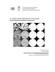
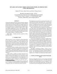
areaExamplesPlot the values in Y as a stacked area plot.Y = [ 1, 5, 3;3, 2, 7;1, 5, 3;2, 6, 1];area(Y)grid oncolormap summerset(gca,'Layer','top')title 'Stacked Area Plot'12Stacked Area Plot10864201 1.5 2 2.5 3 3.5 4See Alsoplot-3

axesPurpose2axesCreate axes graphics objectSyntaxDescriptionaxesaxes('PropertyName',PropertyValue,...)axes(h)h = axes(...)axes is the low-level function for creating axes graphics objects.axes creates an axes graphics object in the current figure using defaultproperty values.axes('PropertyName',PropertyValue,...) creates an axes object having thespecified property values. MATLAB uses default values for any properties thatyou do not explicitly define as arguments.axes(h) makes existing axes h the current axes. It also makes h the first axeslisted in the figure’s Children property and sets the figure’s CurrentAxesproperty to h. The current axes is the target for functions that draw image, line,patch, surface, and text graphics objects.h = axes(...) returns the handle of the created axes object.RemarksMATLAB automatically creates an axes, if one does not already exist, when youissue a command that draws image, light, line, patch, surface, or text graphicsobjects.The axes function accepts property name/property value pairs, structurearrays, and cell arrays as input arguments (see the set and get commands forexamples of how to specify these data types). These properties, which controlvarious aspects of the axes object, are described in the “Axes Properties”section.Use the set function to modify the properties of an existing axes or the getfunction to query the current values of axes properties. Use the gca commandto obtain the handle of the current axes.The axis (not axes) function provides simplified access to commonly usedproperties that control the scaling and appearance of axes.2-4

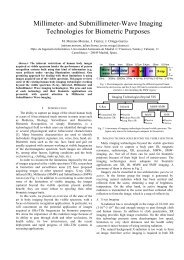
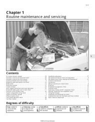
axesWhile the basic purpose of an axes object is to provide a coordinate system forplotted data, axes properties provide considerable control over the wayMATLAB displays data.Stretch-to-FillBy default, MATLAB stretches the axes to fill the axes position rectangle (therectangle defined by the last two elements in the Position property). Thisresults in graphs that use the available space in the rectangle. However, some3-D graphs (such as a sphere) appear distorted because of this stretching, andare better viewed with a specific three-dimensional aspect ratio.Stretch-to-fill is active when the DataAspectRatioMode,PlotBoxAspectRatioMode, and CameraViewAngleMode are all auto (thedefault). However, stretch-to-fill is turned off when the DataAspectRatio,PlotBoxAspectRatio, or CameraViewAngle is user-specified, or when one ormore of the corresponding modes is set to manual (which happensautomatically when you set the corresponding property value).This picture shows the same sphere displayed both with and without thestretch-to-fill. The dotted lines show the axes Position rectangle.18642024681−1 −0.8 −0.6 −0.4 −0.2 0 0.2 0.4 0.6 0.8 1Stretch-to-fill active10.80.60.40.20−0.2−0.4−0.6−0.8−1−1 −0.5 0 0.5 1Stretch-to-fill disabledWhen stretch-to-fill is disabled, MATLAB sets the size of the axes to be as largeas possible within the constraints imposed by the Position rectangle withoutintroducing distortion. In the picture above, the height of the rectangleconstrains the axes size.2-5

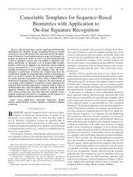
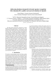
axesExamplesZoomingZoom in using aspect ratio and limits:sphereset(gca,'DataAspectRatio',[1 1 1],...'PlotBoxAspectRatio',[1 1 1],'ZLim',[−0.6 0.6])Zoom in and out using the CameraViewAngle:sphereset(gca,'CameraViewAngle',get(gca,'CameraViewAngle')−5)set(gca,'CameraViewAngle',get(gca,'CameraViewAngle')+5)Note that both examples disable MATLAB’s stretch-to-fill behavior.Positioning the AxesThe axes Position property enables you to define the location of the axeswithin the figure window. For example,h = axes('Position',position_rectangle)creates an axes object at the specified position within the current figure andreturns a handle to it. Specify the location and size of the axes with a rectangledefined by a four-element vector,position_rectangle = [left, bottom, width, height];The left and bottom elements of this vector define the distance from thelower-left corner of the figure to the lower-left corner of the rectangle. Thewidth and height elements define the dimensions of the rectangle. You specifythese values in units determined by the Units property. By default, MATLABuses normalized units where (0,0) is the lower-left corner and (1.0,1.0) is theupper-right corner of the figure window.You can define multiple axes in a single figure window:axes('position',[.1 .1 .8 .6])mesh(peaks(20));axes('position',[.1 .7 .8 .2])pcolor([1:10;1:10]);2-6

axesIn this example, the first plot occupies the bottom two-thirds of the figure, andthe second occupies the top third.21.511 2 3 4 5 6 7 8 9 101050−5−102015105005101520See Alsoaxis, cla, clf, figure, gca, grid, subplot, title, xlabel, ylabel, zlabel,viewObjectHierarchy2-7

axesRootFigureAxesUicontrolUimenuUicontextmenuImageLightLinePatchRectangleSurfaceTextSetting Default PropertiesYou can set default axes properties on the figure and root levels:set(0,'DefaultAxesPropertyName',PropertyValue,...)set(gcf,'DefaultAxesPropertyName',PropertyValue,...)where PropertyName is the name of the axes property and PropertyValue isthe value you are specifying. Use set and get to access axes properties.Property ListThe following table lists all axes properties and provides a brief description ofeach. The property name links take you an expanded description of theproperties.Property Name Property Description Property ValueControlling Style and AppearanceBox Toggle axes plot box on and off Values: on, offDefault: offClippingGridLineStyleThis property has no effect; axes arealways clipped to the figure windowLine style used to draw axes gridlinesValues: −, −−, :, -., noneDefault: : (dotted line)Layer Draw axes above or below graphs Values: bottom, topDefault: bottom2-8

axesProperty Name Property Description Property ValueLineStyleOrderSequence of line styles used formultiline plotsValues: LineSpecDefault: − (solid line for)LineWidth Width of axis lines, in points (1/72"per point)Values: number of pointsDefault: 0.5 pointsSelectionHighlightHighlight axes when selected(Selected property set to on)Values: on, off Default: onTickDir Direction of axis tick marks Values: in, outDefault: in (2-D), out (3-D)TickDirModeTickLengthUse MATLAB or user-specified tickmark directionLength of tick marks normalized toaxis line length, specified astwo-element vectorValues: auto, manualDefault: autoValues: [2-D 3-D]Default: [0.01 0.025}Visible Make axes visible or invisible Values: on, offDefault: onXGrid, YGrid, ZGridToggle grid lines on and off inrespective axisValues: on, offDefault: offGeneral Information About the AxesChildrenCurrentPointHitTestParentHandles of the images, lights, lines,patches, surfaces, and text objectsdisplayed in the axesLocation of last mouse button clickdefined in the axes data unitsSpecify whether axes can become thecurrent object (see figureCurrentObject property)Handle of the figure windowcontaining the axesValues: vector of handlesValues: a 2-by-3 matrixValues: on, offDefault: onValues: scalar figure handle2-9

axesProperty Name Property Description Property ValuePositionSelectedLocation and size of axes within thefigureIndicate whether axes is in a“selected” stateValues: [left bottom widthheight]Default: [0.1300 0.11000.7750 0.8150] innormalized UnitsValues: on, offDefault: onTag User-specified label Values: any stringDefault: '' (empty string)TypeUnitsThe type of graphics object (readonly)Units used to interpret the PositionpropertyValue: the string 'axes'Values: inches, centimeters,characters, normalized,points, pixels Default:normalizedUserData User-specified data Values: any matrixDefault: [] (empty matrix)Selecting Fonts and LabelsFontAngle Select italic or normal font Values: normal, italic,obliqueDefault: normalFontNameFontSizeFont family name (e.g., Helvetica,Courier)Size of the font used for title andlabelsValues: a font supported byyour system or the stringFixedWidthDefault: Typically HelveticaValues: an integer inFontUnits Default: 102-10

axesProperty Name Property Description Property ValueFontUnitsUnits used to interpret the FontSizepropertyValues: points, normalized,inches, centimeters,pixelsDefault: pointsFontWeight Select bold or normal font Values: normal, bold, light,demiDefault: normalTitle Handle of the title text object Values: any valid text objecthandleXLabel, YLabel, ZLabelXTickLabel, YTickLabel,ZTickLabelXTickLabelMode,YTickLabelMode,ZTickLabelModeControlling Axis ScalingHandles of the respective axis labeltext objectsSpecify tick mark labels for therespective axisUse MATLAB or user-specified tickmark labelsValues: any valid text objecthandleValues: matrix of stringsDefaults: numeric valuesselected automatically byMATLABValues: auto, manualDefault: autoXAxisLocation Specify the location of the x-axis Values: top, bottomDefault: bottomYAxisLocation Specify the location of the y-axis Values: right leftDefault: leftXDir, YDir, ZDirXLim, YLim, ZLimSpecify the direction of increasingvalues for the respective axesSpecify the limits to the respectiveaxesValues: normal, reverseDefault: normalValues: [min max]Default: min and maxdetermined automatically byMATLAB2-11

axesProperty Name Property Description Property ValueXLimMode, YLimMode,ZLimModeXScale, YScale, ZScaleXTick, YTick, ZTickXTickMode, YTickMode,ZTickModeControlling the ViewCameraPositionCameraPositionModeUse MATLAB or user-specifiedvalues for the respective axis limitsSelect linear or logarithmic scaling ofthe respective axisSpecify the location of the axis ticksmarksUse MATLAB or user-specifiedvalues for the respective tick marklocationsSpecify the position of point fromwhich you view the sceneUse MATLAB or user-specifiedcamera positionValues: auto, manualDefault: autoValues: linear, logDefault: linear (changed byplotting commands thatcreate nonlinear plots)Values: a vector of datavalues locating tick marksDefault: MATLABautomatically determinestick mark placementValues: auto, manualDefault: autoValues: [x,y,z] axescoordinatesDefault: automaticallydetermined by MATLABValues: auto, manualDefault: autoCameraTarget Center of view pointed to by camera Values: [x,y,z] axescoordinatesDefault: automaticallydetermined by MATLABCameraTargetModeUse MATLAB or user-specifiedcamera targetValues: auto, manualDefault: auto2-12

axesProperty Name Property Description Property ValueCameraUpVector Direction that is oriented up Values: [x,y,z] axescoordinatesDefault: automaticallydetermined by MATLABCameraUpVectorModeUse MATLAB or user-specifiedcamera up vectorValues: auto, manualDefault: autoCameraViewAngle Camera field of view Values: angle in degreesbetween 0 and 180Default: automaticallydetermined by MATLABCameraViewAngleModeUse MATLAB or user-specifiedcamera view angleValues: auto, manualDefault: autoProjection Select type of projection Values: orthographic,perspectiveDefault: orthographicControlling the Axes Aspect RatioDataAspectRatio Relative scaling of data units Values: three relative values[dx dy dz]Default: automaticallydetermined by MATLABDataAspectRatioModeUse MATLAB or user-specified dataaspect ratioValues: auto, manualDefault: autoPlotBoxAspectRatio Relative scaling of axes plot box Values: three relative values[dx dy dz]Default: automaticallydetermined by MATLABPlotBoxAspectRatioModeUse MATLAB or user-specified plotbox aspect ratioValues: auto, manual Default:autoControlling Callback Routine Execution2-13

axesProperty Name Property Description Property ValueBusyActionButtonDownFcnCreateFcnDeleteFcnInterruptibleUIContextMenuSpecify how to handle events thatinterrupt execution callback routinesDefine a callback routine thatexecutes when a button is pressedover the axesDefine a callback routine thatexecutes when an axes is createdDefine a callback routine thatexecutes when an axes is createdControl whether an executingcallback routine can be interruptedAssociate a context menu with theaxesValues: cancel, queueDefault: queueValues: stringDefault: an empty stringValues: stringDefault: an empty stringValues: string Default: anempty stringValues: on, off Default: onValues: handle of aUicontextmenuSpecifying the Rendering ModeDrawModeSpecify the rendering method to usewith the Painters rendererValues: normal, fastDefault: normalTargeting Axes for Graphics DisplayHandleVisibilityNextPlotControl access to a specific axes’handleDetermine the eligibility of the axesfor displaying graphicsValues: on, callback, offDefault: onValues: add, replace,replacechildrenDefault: replaceProperties that Specify ColorAmbientLightColorCLimColor of the background light in asceneControl how data is mapped tocolormapValues: ColorSpecDefault: [1 1 1]Values: [cmin cmax]Default: automaticallydetermined by MATLAB2-14

axesProperty Name Property Description Property ValueCLimModeUse MATLAB or user-specifiedvalues for CLimValues: auto, manualDefault: autoColor Color of the axes background Values: none, ColorSpecDefault: noneColorOrder Line colors used for multiline plots Values: m-by-3 matrix ofRGB valuesDefault: depends on colorscheme usedXColor, YColor, ZColorColors of the axis lines and tickmarksValues: ColorSpecDefault: depends on currentcolor scheme2-15

Axes PropertiesAxesProperties2Axes PropertiesThis section lists property names along with the types of values each accepts.Curly braces { } enclose default values.AmbientLightColorColorSpecThe background light in a scene. Ambient light is a directionless light thatshines uniformly on all objects in the axes. However, if there are no visible lightobjects in the axes, MATLAB does not use AmbientLightColor. If there arelight objects in the axes, the AmbientLightColor is added to the other lightsources.AspectRatio (Obsolete)This property produces a warning message when queried or changed. It hasbeen superseded by the DataAspectRatio[Mode] andPlotBoxAspectRatio[Mode] properties.Boxon | {off}Axes box mode. This property specifies whether to enclose the axes extent in abox for 2-D views or a cube for 3-D views. The default is to not display the box.BusyActioncancel | {queue}Callback routine interruption. The BusyAction property enables you to controlhow MATLAB handles events that potentially interrupt executing callbackroutines. If there is a callback routine executing, subsequently invokedcallback routines always attempt to interrupt it. If the Interruptible propertyof the object whose callback is executing is set to on (the default), theninterruption occurs at the next point where the event queue is processed. If theInterruptible property is off, the BusyAction property (of the object owningthe executing callback) determines how MATLAB handles the event. Thechoices are:• cancel – discard the event that attempted to execute a second callbackroutine.• queue – queue the event that attempted to execute a second callback routineuntil the current callback finishes.ButtonDownFcn stringButton press callback routine. A callback routine that executes whenever youpress a mouse button while the pointer is within the axes, but not over another2-16

Axes Propertiesgraphics object displayed in the axes. For 3-D views, the active area is definedby a rectangle that encloses the axes.Define this routine as a string that is a valid MATLAB expression or the nameof an M-file. The expression executes in the MATLAB workspace.CameraPosition [x, y, z] axes coordinatesThe location of the camera. This property defines the position from which thecamera views the scene. Specify the point in axes coordinates.If you fix CameraViewAngle, you can zoom in and out on the scene by changingthe CameraPosition, moving the camera closer to the CameraTarget to zoom inand farther away from the CameraTarget to zoom out. As you change theCameraPosition, the amount of perspective also changes, if Projection isperspective. You can also zoom by changing the CameraViewAngle; however,this does not change the amount of perspective in the scene.CameraPositionMode {auto} | manualAuto or manual CameraPosition. When set to auto, MATLAB automaticallycalculates the CameraPosition such that the camera lies a fixed distance fromthe CameraTarget along the azimuth and elevation specified by view. Setting avalue for CameraPosition sets this property to manual.CameraTarget [x, y, z] axes coordinatesCamera aiming point. This property specifies the location in the axes that thecamera points to. The CameraTarget and the CameraPosition define the vector(the view axis) along which the camera looks.CameraTargetMode{auto} | manualAuto or manual CameraTarget placement. When this property is auto,MATLAB automatically positions the CameraTarget at the centroid of the axesplotbox. Specifying a value for CameraTarget sets this property to manual.CameraUpVector [x, y, z] axes coordinatesCamera rotation. This property specifies the rotation of the camera around theviewing axis defined by the CameraTarget and the CameraPosition properties.Specify CameraUpVector as a three-element array containing the x, y, and zcomponents of the vector. For example, [0 1 0] specifies the positive y-axis asthe up direction.2-17

Axes PropertiesThe default CameraUpVector is [0 0 1], which defines the positive z-axis as theup direction.CameraUpVectorMode {auto} | manualDefault or user-specified up vector. When CameraUpVectorMode is auto,MATLAB uses a value of [0 0 1] (positive z-direction is up) for 3-D views and[0 1 0] (positive y-direction is up) for 2-D views. Setting a value forCameraUpVector sets this property to manual.CameraViewAngle scalar greater than 0 and less than or equal to180 (angle in degrees)The field of view. This property determines the camera field of view. Changingthis value affects the size of graphics objects displayed in the axes, but does notaffect the degree of perspective distortion. The greater the angle, the larger thefield of view, and the smaller objects appear in the scene.CameraViewAngleMode{auto} | manualAuto or manual CameraViewAngle. When in auto mode, MATLAB setsCameraViewAngle to the minimum angle that captures the entire scene (up to180˚).The following table summarizes MATLAB’s automatic camera behavior.CameraViewAngleCameraTargetCameraPositionBehaviorauto auto auto CameraTarget is set to plot box centroid,CameraViewAngle is set to capture entire scene,CameraPosition is set along the view axis.auto auto manual CameraTarget is set to plot box centroid,CameraViewAngle is set to capture entire scene.auto manual auto CameraViewAngle is set to capture entire scene,CameraPosition is set along the view axis.auto manual manual CameraViewAngle is set to capture entire scene.manual auto auto CameraTarget is set to plot box centroid,CameraPosition is set along the view axis.2-18

Axes PropertiesCameraViewAngleCameraTargetCameraPositionBehaviormanual auto manual CameraTarget is set to plot box centroidmanual manual auto CameraPosition is set along the view axis.manual manual manual All Camera properties are user-specified.Childrenvector of graphics object handlesChildren of the axes. A vector containing the handles of all graphics objectsrendered within the axes (whether visible or not). The graphics objects that canbe children of axes are images, lights, lines, patches, surfaces, and text.The text objects used to label the x-, y-, and z-axes are also children of axes, buttheir HandleVisibility properties are set to callback. This means theirhandles do not show up in the axes Children property unless you set the RootShowHiddenHandles property to on.CLim[cmin, cmax]Color axis limits. A two-element vector that determines how MATLAB mapsthe CData values of surface and patch objects to the figure’s colormap. cmin isthe value of the data mapped to the first color in the colormap, and cmax is thevalue of the data mapped to the last color in the colormap. Data values inbetween are linearly interpolated across the colormap, while data valuesoutside are clamped to either the first or last colormap color, whichever isclosest.When CLimMode is auto (the default), MATLAB assigns cmin the minimumdata value and cmax the maximum data value in the graphics object’s CData.This maps CData elements with minimum data value to the first colormapentry and with maximum data value to the last colormap entry.If the axes contains multiple graphics objects, MATLAB sets CLim to span therange of all objects’ CData.CLimMode{auto} | manualColor axis limits mode. In auto mode, MATLAB sets the CLim property to spanthe CData limits of the graphics objects displayed in the axes. If CLimMode ismanual, MATLAB does not change the value of CLim when the CData limits ofaxes children change. Setting the CLim property sets this property to manual.2-19

Axes PropertiesClipping{on} | offThis property has no effect on axes.Color{none} | ColorSpecColor of the axes back planes. Setting this property to none means the axes istransparent and the figure color shows through. A ColorSpec is athree-element RGB vector or one of MATLAB’s predefined names. Note thatwhile the default value is none, the matlabrc.m file may set the axes color toa specific color.ColorOrder m-by-3 matrix of RGB valuesColors to use for multiline plots. ColorOrder is an m-by-3 matrix of RGB valuesthat define the colors used by the plot and plot3 functions to color each lineplotted. If you do not specify a line color with plot and plot3, these functionscycle through the ColorOrder to obtain the color for each line plotted. To obtainthe current ColorOrder, which may be set during startup, get the propertyvalue:get(gca,'ColorOrder')Note that if the axes NextPlot property is set to replace (the default),high-level functions like plot reset the ColorOrder property beforedetermining the colors to use. If you want MATLAB to use a ColorOrder thatis different from the default, set NextPlot to replacedata. You can also specifyyour own default ColorOrder.CreateFcnstringCallback routine executed during object creation. This property defines acallback routine that executes when MATLAB creates an axes object. You mustdefine this property as a default value for axes. For example, the statement,set(0,'DefaultAxesCreateFcn','set(gca,''Color'',''b'')')defines a default value on the Root level that sets the current axes’ backgroundcolor to blue whenever you (or MATLAB) create an axes. MATLAB executesthis routine after setting all properties for the axes. Setting this property on anexisting axes object has no effect.The handle of the object whose CreateFcn is being executed is accessible onlythrough the Root CallbackObject property, which can be queried using gcbo.2-20

Axes PropertiesCurrentPoint 2-by-3 matrixLocation of last button click, in axes data units. A 2-by-3 matrix containing thecoordinates of two points defined by the location of the pointer. These twopoints lie on the line that is perpendicular to the plane of the screen and passesthrough the pointer. The 3-D coordinates are the points, in the axes coordinatesystem, where this line intersects the front and back surfaces of the axesvolume (which is defined by the axes x, y, and z limits).The returned matrix is of the form:x backy backz backx fronty frontz frontMATLAB updates the CurrentPoint property whenever a button-click eventoccurs. The pointer does not have to be within the axes, or even the figurewindow; MATLAB returns the coordinates with respect to the requested axesregardless of the pointer location.DataAspectRatio[dx dy dz]Relative scaling of data units. A three-element vector controlling the relativescaling of data units in the x, y, and z directions. For example, setting thisproperty t o [1 2 1] causes the length of one unit of data in the x direction tobe the same length as two units of data in the y direction and one unit of datain the z direction.Note that the DataAspectRatio property interacts with thePlotBoxAspectRatio, XLimMode, YLimMode, and ZLimMode properties to controlhow MATLAB scales the x-, y-, and z-axis. Setting the DataAspectRatio willdisable the stretch-to-fill behavior, if DataAspectRatioMode,PlotBoxAspectRatioMode, and CameraViewAngleMode are all auto. Thefollowing table describes the interaction between properties whenstretch-to-fill behavior is disabled.2-21

Axes PropertiesX-, Y-,Z-LimitsDataAspectRatioPlotBoxAspectRatioBehaviorauto auto auto Limits chosen to span data range in alldimensions.auto auto manual Limits chosen to span data range in alldimensions. DataAspectRatio is modified toachieve the requested PlotBoxAspectRatiowithin the limits selected by MATLAB.auto manual auto Limits chosen to span data range in alldimensions. PlotBoxAspectRatio is modified toachieve the requested DataAspectRatio withinthe limits selected by MATLAB.auto manual manual Limits chosen to completely fit and center theplot within the requested PlotBoxAspectRatiogiven the requested DataAspectRatio (this mayproduce empty space around 2 of the 3dimensions).manual auto auto Limits are honored. The DataAspectRatio andPlotBoxAspectRatio are modified as necessary.manual auto manual Limits and PlotBoxAspectRatio are honored.The DataAspectRatio is modified as necessary.manual manual auto Limits and DataAspectRatio are honored. ThePlotBoxAspectRatio is modified as necessary.1 manual2 auto2 or 3manualmanual manual The 2 automatic limits are selected to honor thespecified aspect ratios and limit. See “Examples”manual manual Limits and DataAspectRatio are honored; thePlotBoxAspectRatio is ignored.DataAspectRatioMode{auto} | manualUser or MATLAB controlled data scaling. This property controls whether thevalues of the DataAspectRatio property are user defined or selectedautomatically by MATLAB. Setting values for the DataAspectRatio property2-22

Axes Propertiesautomatically sets this property to manual. Changing DataAspectRatioMode tomanual disables the stretch-to-fill behavior, if DataAspectRatioMode,PlotBoxAspectRatioMode, and CameraViewAngleMode are all auto.DeleteFcnstringDelete axes callback routine. A callback routine that executes when the axesobject is deleted (e.g., when you issue a delete or a close command). MATLABexecutes the routine before destroying the object’s properties so the callbackroutine can query these values.The handle of the object whose DeleteFcn is being executed is accessible onlythrough the Root CallbackObject property, which can be queried using gcbo.DrawMode{normal} | fastRendering method. This property controls the method MATLAB uses to rendergraphics objects displayed in the axes, when the figure Renderer property ispainters.• normal mode draws objects in back to front ordering based on the currentview in order to handle hidden surface elimination and object intersections.• fast mode draws objects in the order in which you specify the drawingcommands, without considering the relationships of the objects in threedimensions. This results in faster rendering because it requires no sorting ofobjects according to location in the view, but may produce undesirableresults because it bypasses the hidden surface elimination and objectintersection handling provided by normal DrawMode.When the figure Renderer is zbuffer, DrawMode is ignored, and hidden surfaceelimination and object intersection handling are always provided.FontAngle{normal} | italic | obliqueSelect italic or normal font. This property selects the character slant for axestext. normal specifies a nonitalic font. italic and oblique specify italic font.FontNameA name such as Courier or the string FixedWidthFont family name. The font family name specifying the font to use for axeslabels. To display and print properly, FontName must be a font that your systemsupports. Note that the x-, y-, and z-axis labels do not display in a new font untilyou manually reset them (by setting the XLabel, YLabel, and ZLabel properties2-23

Axes Propertiesor by using the xlabel, ylabel, or zlabel command). Tick mark labels changeimmediately.Specifying a Fixed-Width FontIf you want an axes to use a fixed-width font that looks good in any locale, youshould set FontName to the string FixedWidth:set(axes_handle,'FontName','FixedWidth')This eliminates the need to hardcode the name of a fixed-width font, which maynot display text properly on systems that do not use ASCII character encoding(such as in Japan where multibyte character sets are used). A properly writtenMATLAB application that needs to use a fixed-width font should set FontNameto FixedWidth (note that this string is case sensitive) and rely onFixedWidthFontName to be set correctly in the end-user’s environment.End users can adapt a MATLAB application to different locales or personalenvironments by setting the root FixedWidthFontName property to theappropriate value for that locale from startup.m.Note that setting the root FixedWidthFontName property causes an immediateupdate of the display to use the new font.FontSizeFont size specified in FontUnitsFont size. An integer specifying the font size to use for axes labels and titles, inunits determined by the FontUnits property. The default point size is 12. Thex-, y-, and z-axis text labels do not display in a new font size until you manuallyreset them (by setting the XLabel, YLabel, or ZLabel properties or by using thexlabel, ylabel, or zlabel command). Tick mark labels change immediately.FontUnits {points} | normalized | inches |centimeters | pixelsUnits used to interpret the FontSize property. When set to normalized,MATLAB interprets the value of FontSize as a fraction of the height of theaxes. For example, a normalized FontSize of 0.1 sets the text characters to afont whose height is one tenth of the axes’ height. The default units (points),are equal to 1/72 of an inch.FontWeight{normal} | bold | light | demiSelect bold or normal font. The character weight for axes text. The x-, y-, andz-axis text labels do not display in bold until you manually reset them (by2-24

Axes Propertiessetting the XLabel, YLabel, and ZLabel properties or by using the xlabel,ylabel, or zlabel commands). Tick mark labels change immediately.GridLineStyle− | − −| {:} | −. | noneLine style used to draw grid lines. The line style is a string consisting of acharacter, in quotes, specifying solid lines (−), dashed lines (−−), dottedlines(:), or dash-dot lines (−.). The default grid line style is dotted. To turn ongrid lines, use the grid command.HandleVisibility{on} | callback | offControl access to object’s handle by command-line users and GUIs. Thisproperty determines when an object’s handle is visible in its parent’s list ofchildren. HandleVisibility is useful for preventing command-line users fromaccidentally drawing into or deleting a figure that contains only user interfacedevices (such as a dialog box).Handles are always visible when HandleVisibility is on.Setting HandleVisibility to callback causes handles to be visible fromwithin callback routines or functions invoked by callback routines, but not fromwithin functions invoked from the command line. This provides a means toprotect GUIs from command-line users, while allowing callback routines tohave complete access to object handles.Setting HandleVisibility to off makes handles invisible at all times. Thismay be necessary when a callback routine invokes a function that mightpotentially damage the GUI (such as evaluating a user-typed string) and sotemporarily hides its own handles during the execution of that function.When a handle is not visible in its parent’s list of children, it cannot bereturned by functions that obtain handles by searching the object hierarchy orquerying handle properties. This includes get, findobj, gca, gcf, gco, newplot,cla, clf, and close.When a handle’s visibility is restricted using callback or off, the object’shandle does not appear in its parent’s Children property, figures do not appearin the Root’s Currentfigure property, objects do not appear in the Root’sCallbackObject property or in the figure’s CurrentObject property, and axesdo not appear in their parent’s Currentaxes property.2-25

Axes PropertiesYou can set the Root ShowHiddenHandles property to on to make all handlesvisible, regardless of their HandleVisibility settings (this does not affect thevalues of the HandleVisibility properties).Handles that are hidden are still valid. If you know an object’s handle, you canset and get its properties, and pass it to any function that operates on handles.HitTest{on} | offSelectable by mouse click. HitTest determines if the axes can become thecurrent object (as returned by the gco command and the figure CurrentObjectproperty) as a result of a mouse click on the axes. If HiTest is off, clicking onthe axes selects the object below it (which is usually the figure containing it).Interruptible{on} | offCallback routine interruption mode. The Interruptible property controlswhether an axes callback routine can be interrupted by subsequently invokedcallback routines. Only callback routines defined for the ButtonDownFcn areaffected by the Interruptible property. MATLAB checks for events that caninterrupt a callback routine only when it encounters a drawnow, figure,getframe, or pause command in the routine. See the BusyAction property forrelated information.Setting Interruptible to on allows any graphics object’s callback routine tointerrupt callback routines originating from an axes property. Note thatMATLAB does not save the state of variables or the display (e.g., the handlereturned by the gca or gcf command) when an interruption occurs.Layer{bottom} | topDraw axis lines below or above graphics objects. This property determines ifaxis lines and tick marks draw on top or below axes children objects for any 2-Dview (i.e., when you are looking along the x-, y-, or z-axis). This is useful forplacing grid lines and tick marks on top of images.LineStyleOrderLineSpecOrder of line styles and markers used in a plot. This property specifies whichline styles and markers to use and in what order when creating multiple-lineplots. For example,set(gca,'LineStyleOrder', '−*|:|o')2-26

Axes Propertiessets LineStyleOrder to solid line with asterisk marker, dotted line, and hollowcircle marker. The default is (−), which specifies a solid line for all data plotted.Alternatively, you can create a cell array of character strings to define the linestyles:set(gca,'LineStyleOrder',{'−*',':','o'})MATLAB supports four line styles, which you can specify any number of timesin any order. MATLAB cycles through the line styles only after using all colorsdefined by the ColorOrder property. For example, the first eight lines plotteduse the different colors defined by ColorOrder with the first line style.MATLAB then cycles through the colors again, using the second line stylespecified, and so on.You can also specify line style and color directly with the plot and plot3functions or by altering the properties of the line objects.Note that, if the axes NextPlot property is set to replace (the default),high-level functions like plot reset the LineStyleOrder property beforedetermining the line style to use. If you want MATLAB to use aLineStyleOrder that is different from the default, set NextPlot toreplacedata. You can also specify your own default LineStyleOrder.LineWidthlinewidth in pointsWidth of axis lines. This property specifies the width, in points, of the x-, y-, andz-axis lines. The default line width is 0.5 points (1 point = 1 / 72 inch).NextPlotadd | {replace} | replacechildrenWhere to draw the next plot. This property determines how high-level plottingfunctions draw into an existing axes.• add — use the existing axes to draw graphics objects.• replace — reset all axes properties, except Position, to their defaults anddelete all axes children before displaying graphics (equivalent to cla reset).• replacechildren — remove all child objects, but do not reset axes properties(equivalent to cla).The newplot function simplifies the use of the NextPlot property and is usedby M-file functions that draw graphs using only low-level object creationroutines. See the M-file pcolor.m for an example. Note that figure graphicsobjects also have a NextPlot property.2-27

Axes PropertiesParentfigure handleAxes parent. The handle of the axes’ parent object. The parent of an axes objectis the figure in which it is displayed. The utility function gcf returns the handleof the current axes’ Parent. You can reparent axes to other figure objects.PlotBoxAspectRatio[px py pz]Relative scaling of axes plotbox. A three-element vector controlling the relativescaling of the plot box in the x-, y-, and z-directions. The plot box is a boxenclosing the axes data region as defined by the x-, y-, and z-axis limits.Note that the PlotBoxAspectRatio property interacts with theDataAspectRatio, XLimMode, YLimMode, and ZLimMode properties to control theway graphics objects are displayed in the axes. Setting thePlotBoxAspectRatio disables stretch-to-fill behavior, ifDataAspectRatioMode, PlotBoxAspectRatioMode, and CameraViewAngleModeare all auto.PlotBoxAspectRatioMode{auto} | manualUser or MATLAB controlled axis scaling. This property controls whether thevalues of the PlotBoxAspectRatio property are user defined or selectedautomatically by MATLAB. Setting values for the PlotBoxAspectRatioproperty automatically sets this property to manual. Changing thePlotBoxAspectRatioMode to manual disables stretch-to-fill behavior, ifDataAspectRatioMode, PlotBoxAspectRatioMode, and CameraViewAngleModeare all auto.Positionfour-element vectorPosition of axes. A four-element vector specifying a rectangle that locates theaxes within the figure window. The vector is of the form:[left bottom width height]where left and bottom define the distance from the lower-left corner of thefigure window to the lower-left corner of the rectangle. width and height arethe dimensions of the rectangle. All measurements are in units specified by theUnits property.When axes stretch-to-fill behavior is enabled (when DataAspectRatioMode,PlotBoxAspectRatioMode, CameraViewAngleMode are all auto), the axes arestretched to fill the Position rectangle. When stretch-to-fill is disabled, the2-28

Axes Propertiesaxes are made as large as possible, while obeying all other properties, withoutextending outside the Position rectangleProjection{orthographic} | perspectiveType of projection. This property selects between two projection types:• orthographic – This projection maintains the correct relative dimensions ofgraphics objects with regard to the distance a given point is from the viewer.Parallel lines in the data are drawn parallel on the screen.• perspective – This projection incorporates foreshortening, which allows youto perceive depth in 2-D representations of 3-D objects. Perspectiveprojection does not preserve the relative dimensions of objects; a distant linesegment displays smaller than a nearer line segment of the same length.Parallel lines in the data may not appear parallel on screen.Selectedon | offIs object selected. When you set this property to on, MATLAB displays selection“handles” at the corners and midpoints if the SelectionHighlight property isalso on (the default). You can, for example, define the ButtonDownFcn callbackroutine to set this property to on, thereby indicating that the axes has beenselected.SelectionHighlight{on} | offObjects highlight when selected. When the Selected property is on, MATLABindicates the selected state by drawing four edge handles and four cornerhandles. When SelectionHighlight is off, MATLAB does not draw thehandles.TagstringUser-specified object label. The Tag property provides a means to identifygraphics objects with a user-specified label. This is particularly useful whenconstructing interactive graphics programs that would otherwise need todefine object handles as global variables or pass them as arguments betweencallback routines.For example, suppose you want to direct all graphics output from an M-file toa particular axes, regardless of user actions that may have changed the currentaxes. To do this, identify the axes with a Tag:axes('Tag','Special Axes')2-29

Axes PropertiesThen make that axes the current axes before drawing by searching for the Tagwith findobj:axes(findobj('Tag','Special Axes'))TickDirin | outDirection of tick marks. For 2-D views, the default is to direct tick marksinward from the axis lines; 3-D views direct tick marks outward from the axisline.TickDirMode{auto} | manualAutomatic tick direction control. In auto mode, MATLAB directs tick marksinward for 2-D views and outward for 3-D views. When you specify a setting forTickDir, MATLAB sets TickDirMode to manual. In manual mode, MATLABdoes not change the specified tick direction.TickLength[2DLength 3DLength]Length of tick marks. A two-element vector specifying the length of axes tickmarks. The first element is the length of tick marks used for 2-D views and thesecond element is the length of tick marks used for 3-D views. Specify tick marklengths in units normalized relative to the longest of the visible X-, Y-, or Z-axisannotation lines.Titlehandle of text objectAxes title. The handle of the text object that is used for the axes title. You canuse this handle to change the properties of the title text or you can set Title tothe handle of an existing text object. For example, the following statementchanges the color of the current title to red:set(get(gca,'Title'),'Color','r')To create a new title, set this property to the handle of the text object you wantto use:set(gca,'Title',text('String','New Title','Color','r'))However, it is generally simpler to use the title command to create or replacean axes title:title('New Title','Color','r')2-30

Axes PropertiesTypestring (read only)Type of graphics object. This property contains a string that identifies the classof graphics object. For axes objects, Type is always set to 'axes'.UIContextMenuhandle of a uicontextmenu objectAssociate a context menu with the axes. Assign this property the handle of aUicontextmenu object created in the axes’ parent figure. Use theuicontextmenu function to create the context menu. MATLAB displays thecontext menu whenever you right-click over the axes.Units inches | centimeters | {normalized} |points | pixels | charactersPosition units. The units used to interpret the Position property. All units aremeasured from the lower-left corner of the figure window.• normalized units map the lower-left corner of the figure window to (0,0) andthe upper-right corner to (1.0, 1.0).• inches, centimeters, and points are absolute units (one point equals 1 / 72 ofan inch).• Character units are defined by characters from the default system font; thewidth of one character is the width of the letter x, the height of one characteris the distance between the baselines of two lines of text.UserDatamatrixUser specified data. This property can be any data you want to associate withthe axes object. The axes does not use this property, but you can access it usingthe set and get functions.ViewObsoleteThe functionality provided by the View property is now controlled by the axescamera properties – CameraPosition, CameraTarget, CameraUpVector, andCameraViewAngle. See the view command.Visible{on} | offVisibility of axes. By default, axes are visible. Setting this property to offprevents axis lines, tick marks, and labels from being displayed. The visibleproperty does not affect children of axes.2-31

Axes PropertiesXAxisLocationtop | {bottom}Location of x-axis tick marks and labels. This property controls whereMATLAB displays the x-axis tick marks and labels. Setting this property to topmoves the x-axis to the top of the plot from its default position at the bottom.YAxisLocationright | {left}Location of y-axis tick marks and labels. This property controls whereMATLAB displays the y-axis tick marks and labels. Setting this property toright moves the y-axis to the right side of the plot from its default position onthe left side. See the plotyy function for a simple way to use two y-axes.Properties That Control the X-, Y-, or Z-AxisXColor, YColor, ZColorColorSpecColor of axis lines. A three-element vector specifying an RGB triple, or apredefined MATLAB color string. This property determines the color of the axislines, tick marks, tick mark labels, and the axis grid lines of the respective x-,y-, and z-axis. The default axis color is white. See ColorSpec for details onspecifying colors.XDir, YDir, ZDir{normal} | reverseDirection of increasing values. A mode controlling the direction of increasingaxis values. axes form a right-hand coordinate system. By default:• x-axis values increase from left to right. To reverse the direction of increasingx values, set this property to reverse.• y-axis values increase from bottom to top (2-D view) or front to back (3-Dview). To reverse the direction of increasing y values, set this property toreverse.• z-axis values increase pointing out of the screen (2-D view) or from bottom totop (3-D view). To reverse the direction of increasing z values, set thisproperty to reverse.XGrid, YGrid, ZGridon | {off}Axis gridline mode. When you set any of these properties to on, MATLAB drawsgrid lines perpendicular to the respective axis (i.e., along lines of constant x, y,or z values). Use the grid command to set all three properties on or off at once.2-32

Axes PropertiesXLabel, YLabel, ZLabel handle of text objectAxis labels. The handle of the text object used to label the x, y, or z-axis,respectively. To assign values to any of these properties, you must obtain thehandle to the text string you want to use as a label. This statement defines atext object and assigns its handle to the XLabel property:set(gca,'Xlabel',text('String','axis label'))MATLAB places the string 'axis label' appropriately for an x-axis label. Anytext object whose handle you specify as an XLabel, YLabel, or ZLabel propertyis moved to the appropriate location for the respective label.Alternatively, you can use the xlabel, ylabel, and zlabel functions, whichgenerally provide a simpler means to label axis lines.XLim, YLim, ZLim[minimum maximum]Axis limits. A two-element vector specifying the minimum and maximumvalues of the respective axis.Changing these properties affects the scale of the x-, y-, or z-dimension as wellas the placement of labels and tick marks on the axis. The default values forthese properties are [0 1].XLimMode, YLimMode, ZLimMode{auto} | manualMATLAB or user-controlled limits. The axis limits mode determines whetherMATLAB calculates axis limits based on the data plotted (i.e., the XData,YData, or ZData of the axes children) or uses the values explicitly set with theXLim, YLim, or ZLim property, in which case, the respective limits mode is set tomanual.XScale, YScale, ZScale{linear} | logAxis scaling. Linear or logarithmic scaling for the respective axis. See alsologlog, semilogx, and semilogy.XTick, YTick, ZTick vector of data values locating tick marksTick spacing. A vector of x-, y-, or z-data values that determine the location oftick marks along the respective axis. If you do not want tick marks displayed,set the respective property to the empty vector, [ ]. These vectors must containmonotonically increasing values.2-33

Axes PropertiesXTickLabel, YTickLabel, ZTickLabelstringTick labels. A matrix of strings to use as labels for tick marks along therespective axis. These labels replace the numeric labels generated byMATLAB. If you do not specify enough text labels for all the tick marks,MATLAB uses all of the labels specified, then reuses the specified labels.For example, the statement,set(gca,'XTickLabel',{'One';'Two';'Three';'Four'})labels the first four tick marks on the x-axis and then reuses the labels until allticks are labeled.Labels can be specified as cell arrays of strings, padded string matrices, stringvectors separated by vertical slash characters, or as numeric vectors (whereeach number is implicitly converted to the equivalent string using num2str). Allof the following are equivalent:set(gca,'XTickLabel',{'1';'10';'100'})set(gca,'XTickLabel','1|10|100')set(gca,'XTickLabel',[1;10;100])set(gca,'XTickLabel',['1 ';'10 ';'100'])Note that tick labels do not interpret TeX character sequences (however, theTitle, XLabel, YLabel, and ZLabel properties do).XTickMode, YTickMode, ZTickMode{auto} | manualMATLAB or user controlled tick spacing. The axis tick modes determinewhether MATLAB calculates the tick mark spacing based on the range of datafor the respective axis (auto mode) or uses the values explicitly set for any ofthe XTick, YTick, and ZTick properties (manual mode). Setting values for theXTick, YTick, or ZTick properties sets the respective axis tick mode to manual.XTickLabelMode, YTickLabelMode, ZTickLabelMode{auto} | manualMATLAB or user determined tick labels. The axis tick mark labeling modedetermines whether MATLAB uses numeric tick mark labels that span therange of the plotted data (auto mode) or uses the tick mark labels specified withthe XTickLabel, YTickLabel, or ZTickLabel property (manual mode). Settingvalues for the XTickLabel, YTickLabel, or ZTickLabel property sets therespective axis tick label mode to manual.2-34

axisPurpose2axisAxis scaling and appearanceSyntaxaxis([xmin xmax ymin ymax])axis([xmin xmax ymin ymax zmin zmax])v = axisaxis autoaxis manualaxis tightaxis fillaxis ijaxis xyaxis equalaxis imageaxis squareaxis vis3daxis normalaxis offaxis on[mode,visibility,direction] = axis('state')Descriptionaxis manipulates commonly used axes properties. (See Algorithm section.)axis([xmin xmax ymin ymax]) sets the limits for the x- and y-axis of thecurrent axes.axis([xmin xmax ymin ymax zmin zmax]) sets the limits for the x-, y-, andz-axis of the current axes.v = axis returns a row vector containing scaling factors for the x-, y-, andz-axis. v has four or six components depending on whether the current axes is2-D or 3-D, respectively. The returned values are the current axes’ XLim, Ylim,and ZLim properties.2-35

axisaxis auto sets MATLAB to its default behavior of computing the current axes’limits automatically, based on the minimum and maximum values of x, y, andz data. You can restrict this automatic behavior to a specific axis. For example,axis 'auto x' computes only the x-axis limits automatically; axis 'auto yz'computes the y- and z-axis limits automatically.axis manual and axis(axis) freezes the scaling at the current limits, so thatif hold is on, subsequent plots use the same limits. This sets the XLimMode,YLimMode, and ZLimMode properties to manual.axis tight sets the aspect ratio so that the data units are the same in everydirection. This differs from axis equal because the plot box aspect ratioautomatically adjusts.axis fill sets the axis limits to the range of the data.axis ij places the coordinate system origin in the upper-left corner. Thei-axis is vertical, with values increasing from top to bottom. The j-axis ishorizontal with values increasing from left to right.axis xy draws the graph in the default Cartesian axes format with thecoordinate system origin in the lower-left corner. The x-axis is horizontal withvalues increasing from left to right. The y-axis is vertical with values increasingfrom bottom to top.axis equal sets the aspect ratio so that the data units are the same in everydirection. The aspect ratio of the x-, y-, and z-axis is adjusted automaticallyaccording to the range of data units in the x, y, and z directions.axis image is the same as axis equal except that the plot box fits tightlyaround the data.axis square makes the current axes region square (or cubed whenthree-dimensional). MATLAB adjusts the x-axis, y-axis, and z-axis so that theyhave equal lengths and adjusts the increments between data units accordingly.axis vis3d freezes aspect ratio properties to enable rotation of 3-D objectsand overrides stretch-to-fill.2-36

axisaxis normal automatically adjusts the aspect ratio of the axes and the aspectratio of the data units represented on the axes to fill the plot box.axis off turns off all axis lines, tick marks, and labels.axis on turns on all axis lines, tick marks, and labels.[mode,visibility,direction] = axis('state') returns three stringsindicating the current setting of axes properties:Output ArgumentmodevisibilitydirectionStrings Returned'auto' | 'manual''on' | 'off''xy' | 'ij'mode is auto if XLimMode, YLimMode, and ZLimMode are all set to auto. IfXLimMode, YLimMode, or ZLimMode is manual, mode is manual.ExamplesThe statementsx = 0:.025:pi/2;plot(x,tan(x),'-ro')2-37

axisuse the automatic scaling of the y-axis based on ymax = tan(1.57), which iswell over 1000:14001200100080060040020000 0.2 0.4 0.6 0.8 1 1.2 1.4 1.62-38

axisThe right figure shows a more satisfactory plot after typingaxis([0 pi/2 0 5])54.543.532.521.510.500 0.5 1 1.5AlgorithmWhen you specify minimum and maximum values for the x-, y-, and z-axes,axis sets the XLim, Ylim, and ZLim properties for the current axes to therespective minimum and maximum values in the argument list. Additionally,the XLimMode, YLimMode, and ZLimMode properties for the current axes are setto manual.axis auto sets the current axes’ XLimMode, YLimMode, and ZLimMode propertiesto 'auto'.axis manual sets the current axes’ XLimMode, YLimMode, and ZLimModeproperties to 'manual'.The following table shows the values of the axes properties set by axis equal,axis normal, axis square, and axis image.2-39

axisAxes Property axis equal axis normal axis square axis tightequalDataAspectRatio [1 1 1] not set not set [1 1 1]DataAspectRatioMode manual auto auto manualPlotBoxAspectRatio [3 4 4] not set [1 1 1] autoPlotBoxAspectRatioMode manual auto manual autoStretch-to-fill disabled active disabled disabledSee Alsoaxes, get, grid, set, subplotProperties of axes graphics objects2-40

ar, barhPurpose2bar, barhBar chartSyntaxbar(Y)bar(x,Y)bar(...,width)bar(...,'style')bar(...,LineSpec)[xb,yb] = bar(...)h = bar(...)barh(...)[xb,yb] = barh(...)h = barh(...)DescriptionA bar chart displays the values in a vector or matrix as horizontal or verticalbars.bar(Y) draws one bar for each element in Y. If Y is a matrix, bar groups thebars produced by the elements in each row. The x-axis scale ranges from 1 tolength(Y) when Y is a vector, and 1 to size(Y,1), which is the number of rows,when Y is a matrix.bar(x,Y) draws a bar for each element in Y at locations specified in x, where xis a monotonically increasing vector defining the x-axis intervals for thevertical bars. If Y is a matrix, bar clusters the elements in the same row in Y atlocations corresponding to an element in x.bar(...,width) sets the relative bar width and controls the separation of barswithin a group. The default width is 0.8, so if you do not specify x, the barswithin a group have a slight separation. If width is 1, the bars within a grouptouch one another.2-41

ar, barhbar(...,'style') specifies the style of the bars. 'style' is 'group' or'stack'. 'group' is the default mode of display.• 'group' displays n groups of m vertical bars, where n is the number of rowsand m is the number of columns in Y. The group contains one bar per columnin Y.• 'stack' displays one bar for each row in Y. The bar height is the sum of theelements in the row. Each bar is multi-colored, with colors corresponding todistinct elements and showing the relative contribution each row elementmakes to the total sum.bar(...,LineSpec) displays all bars using the color specified by LineSpec.[xb,yb] = bar(...) returns vectors that you plot using plot(xb,yb) orpatch(xb,yb,C). This gives you greater control over the appearance of a graph,for example, to incorporate a bar chart into a more elaborate plot statement.h = bar(...) returns a vector of handles to patch graphics objects. barcreates one patch graphics object per column in Y.barh(...), [xb,yb] = barh(...), and h = barh(...) create horizontalbars. Y determines the bar length. The vector x is a monotonic vector definingthe y-axis intervals for horizontal bars.2-42

ar, barhExamplesPlot a bell shaped curve:x = –2.9:0.2:2.9;bar(x,exp(–x.*x))colormap hsv10.90.80.70.60.50.40.30.20.10−3 −2 −1 0 1 2 3Create four subplots showing the effects of various bar arguments:Y = round(rand(5,3)*10);subplot(2,2,1)bar(Y,'group')title 'Group'subplot(2,2,2)bar(Y,'stack')title 'Stack'subplot(2,2,3)barh(Y,'stack')title 'Stack'2-43

ar, barhsubplot(2,2,4)bar(Y,1.5)title 'Width = 1.5'10Group25Stack8206154102501 2 3 4 501 2 3 4 5Stack10Width = 1.55432186420 5 10 15 20 2501 2 3 4 5See Alsobar3, ColorSpec, patch, stairs, hist2-44

ar3, bar3hPurpose2bar3, bar3hThree-dimensional bar chartSyntaxbar3(Y)bar3(x,Y)bar3(...,width)bar3(...,'style')bar3(...,LineSpec)h = bar3(...)bar3h(...)h = bar3h(...)Descriptionbar3 and bar3h draw three-dimensional vertical and horizontal bar charts.bar3(Y) draws a three-dimensional bar chart, where each element in Ycorresponds to one bar. When Y is a vector, the x-axis scale ranges from 1 tolength(Y). When Y is a matrix, the x-axis scale ranges from 1 to size(Y,2),which is the number of columns, and the elements in each row are groupedtogether.bar3(x,Y) draws a bar chart of the elements in Y at the locations specified inx, where x is a monotonic vector defining the y-axis intervals for vertical bars.If Y is a matrix, bar3 clusters elements from the same row in Y at locationscorresponding to an element in x. Values of elements in each row are groupedtogether.bar3(...,width) sets the width of the bars and controls the separation of barswithin a group. The default width is 0.8, so if you do not specify x, bars withina group have a slight separation. If width is 1, the bars within a group touchone another.bar3(...,'style') specifies the style of the bars. 'style' is 'detached','grouped', or 'stacked'. 'detached' is the default mode of display.• 'detached' displays the elements of each row in Y as separate blocks behindone another in the x direction.2-45

ar3, bar3h• 'grouped' displays n groups of m vertical bars, where n is the number ofrows and m is the number of columns in Y. The group contains one bar percolumn in Y.• 'stacked' displays one bar for each row in Y. The bar height is the sum ofthe elements in the row. Each bar is multi-colored, with colors correspondingto distinct elements and showing the relative contribution each row elementmakes to the total sum.bar3(...,LineSpec) displays all bars using the color specified by LineSpec.h = bar3(...) returns a vector of handles to patch graphics objects. bar3creates one patch object per column in Y.bar3h(...) and h = bar3h(...) create horizontal bars. Y determines the barlength. The vector x is a monotonic vector defining the y-axis intervals forhorizontal bars.ExamplesThis example creates six subplots showing the effects of different argumentsfor bar3. The data Y is a seven-by-three matrix generated using the coolcolormap:Y = cool(7);subplot(3,2,1)bar3(Y,’detached’)title(‘Detached’)subplot(3,2,2)bar3(Y,0.25,’detached’)title(‘Width = 0.25’)subplot(3,2,3)bar3(Y,’grouped’)title(‘Grouped’)2-46

ar3, bar3hsubplot(3,2,4)bar3(Y,0.5,’grouped’)title(‘Width = 0.5’)subplot(3,2,5)bar3(Y,’stacked’)title(‘Stacked’)subplot(3,2,6)bar3(Y,0.3,’stacked’)title(‘Width = 0.3’)colormap([1 0 0;0 1 0;0 0 1])2-47

ar3, bar3hDetachedWidth = 0.25110.50.5001 2 3 4 5 6 71 2 3 4 5 6 71Grouped1Width = 0.50.50.5001 2 3 4 5 6 71 2 3 4 5 6 72Stacked2Width = 0.31.51.5110.50.5001 2 3 4 5 6 71 2 3 4 5 6 7See Alsobar, LineSpec, patch2-48

oxPurpose2boxControl axes borderSyntaxDescriptionbox onbox offboxbox on displays the boundary of the current axes.box off does not display the boundary of the current axes.box toggles the visible state of the current axes’ boundary.AlgorithmSee AlsoThe box function sets the axes Box property to on or off.axes2-49

ightenPurpose2brightenBrighten or darken colormapSyntaxDescriptionbrighten(beta)brighten(h,beta)newmap = brighten(beta)newmap = brighten(cmap,beta)brighten increases or decreases the color intensities in a colormap. Themodified colormap is brighter if 0 < beta < 1 and darker if –1 < beta < 0.brighten(beta) replaces the current colormap with a brighter or darkercolormap of essentially the same colors. brighten(beta), followed bybrighten(–beta), where beta < 1, restores the original map.brighten(h,beta) brightens all objects that are children of the figure havingthe handle h.newmap = brighten(beta) returns a brighter or darker version of the currentcolormap without changing the display.newmap = brighten(cmap,beta) returns a brighter or darker version of thecolormap cmap without changing the display.ExamplesBrighten and then darken the current colormap:beta = .5; brighten(beta);beta = —.5; brighten(beta);AlgorithmThe values in the colormap are raised to the power of gamma, where gamma is⎧1 – β, β > 0γ = ⎨ 1⎩------------, β ≤ 01 + βbrighten has no effect on graphics objects defined with true color.See Alsocolormap, rgbplot2-50

camdollyPurpose2camdollyMove the camera position and targetSyntaxDescriptioncamdolly(dx,dy,dz)camdolly(dx,dy,dz,'targetmode')camdolly(dx,dy,dz,'targetmode','coordsys')camdolly(axes_handle,...)camdolly moves the camera position and the camera target by the specifiedamounts.camdolly(dx,dy,dz) moves the camera position and the camera target by thespecified amounts (see “Coordinate Systems”).camdolly(dx,dy,dz,'targetmode') The targetmode argument can take ontwo values that determine how MATLAB moves the camera:• movetarget (default) – move both the camera and the target• fixtarget – move only the cameracamdolly(dx,dy,dz,'targetmode','coordsys') The coordsys argumentcan take on three values that determine how MATLAB interprets dx, dy, anddz:Coordinate Systems• camera (default) – move in the camera’s coordinate system. dx moves left/right, dy moves down/up, and dz moves along the viewing axis. The units arenormalized to the scene.For example, setting dx to 1 moves the camera to the right, which pushes thescene to the left edge of the box formed by the axes position rectangle. Anegative value moves the scene in the other direction. Setting dz to 0.5moves the camera to a position halfway between the camera position and thecamera target• pixels – interpret dx and dy as pixel offsets. dz is ignored.• data – interpret dx, dy, and dz as offesets in axes data coordinates.camdolly(axes_handle,...) operates on the axes identified by the firstargument, axes_handle. When you do not specify an axes handle, camdollyoperates on the current axes.2-51

camdollyRemarksExamplescamdolly sets the axes CameraPosition and CameraTarget properties, which inturn causes the CameraPositionMode and CameraTargetMode properties to beset to manual.This example moves the camera along the x- and y-axes in a series of steps.surf(peaks)axis vis3dt = 0:pi/20:2*pi;dx = sin(t)./40;dy = cos(t)./40;for i = 1:length(t);camdolly(dx(i),dy(i),0)drawnowendSee Alsoaxes, campos, camproj, camtarget, camup, camvaThe axes properties CameraPosition, CameraTarget, CameraUpVector,CameraViewAngle, ProjectionThe “Camera Properties” section in the online Using MATLAB Graphics topicaccessed via the helpdesk command.2-52

camlightPurpose2camlightCreate or move a light object in camera coordinatesSyntaxDescriptioncamlight headlightcamlight rightcamlight leftcamlightcamlight(az,el)camlight(...‘style’)camlight(light_handle,...)light_handle = camlight(...)camlight('headlight') creates a light at the camera position.camlight('right') creates a light right and up from camera.camlight('left') creates a light left and up from camera.camlight with no arguments is the same as camlight('right').camlight(az,el) creates a light at the specified azimuth (az) and elevation(el) with respect to the camera position. The camera target is the center ofrotation and az and el are in degrees.camlight(...,'style') The style argument can take on the two values:• local (default) – the light is a point source that radiates from the location inall directions.• infinite – the light shines in parallel rays.camlight(light_handle,...) uses the light specified in light_handle.light_handle = camlight(...) returns the light’s handle.Remarkscamlight sets the light object Position and Style properties. A light createdwith camlight will not track the camera. In order for the light to stay in aconstant position relative to the camera, you must call camlight whenever youmove the camera.2-53

camlightExamplesThis example creates a light positioned to the left of the camera and thenrepositions the light each time the camera is moved:surf(peaks)axis vis3dh = camlight(‘left’);for i = 1:20;camorbit(10,0)camlight(h, ‘left’)drawnow;end2-54

camlookatPurpose2camlookatPosition the camera to view an object or group of objectsSyntaxDescriptioncamlookat(object_handles)camlookat(axes_handle)camlookatcamlookat(object_handles) views the objects identified in the vectorobject_handles. The vector can contain the handles of axes children.camlookat(axes_handle) views the objects that are children of the axesidentified by axes_handle.camlookat views the objects that are in the current axes.RemarksExamplescamlookat moves the camera position and camera target while preserving therelative view direction and camera view angle. The object (or objects) beingviewed roughly fill the axes position rectangle.camlookat sets the axes CameraPosition and CameraTarget properties.This example creates three spheres at different locations and thenprogressively positions the camera so that each sphere is the object aroundwhich the scene is composed:[x y z] = sphere;s1 = surf(x,y,z);hold ons2 = surf(x+3,y,z+3);s3 = surf(x,y,z+6);daspect([1 1 1])view(30,10)camproj perspectivecamlookat(gca) % Compose the scene around the current axespause(2)camlookat(s1) % Compose the scene around sphere s1pause(2)camlookat(s2) % Compose the scene around sphere s2pause(2)camlookat(s3) % Compose the scene around sphere s3pause(2)camlookat(gca)2-55

camlookatSee Alsocampos, camtarget2-56

camorbitPurpose2camorbitRotate the camera position around the camera targetSyntaxDescriptioncamorbit(dtheta,dphi)camorbit(dtheta,dphi,'coordsys')camorbit(dtheta,dphi,'coordsys','direction')camorbit(axes_handle,...)camorbit(dtheta,dphi) rotates the camera position around the cameratarget by the amounts specified in dtheta and dphi (both in degrees). dthetais the horizontal rotation and dphi is the vertical rotation.camorbit(dtheta,dphi,'coordsys') The coordsys argument determinesthe center of rotation. It can take on two values:• data (default) – rotate the camera around an axis defined by the cameratarget and the direction (default is the positive z direction).• camera – rotate the camera about the point defined by the camera target.camorbit(dtheta,dphi,'coordsys','direction') The directionargument, in conjunction with the camera target, defines the axis of rotationfor the data coordinate system. Specify direction as a three-element vectorcontaining the x, y, and z-components of the direction or one of the characters,x, y, or z, to indicate [1 0 0], [0 1 0], or [0 0 1] respectively.camorbit(axes_handle,...) operates on the axes identified by the firstargument, axes_handle. When you do not specify an axes handle, camorbitoperates on the current axes.ExamplesCompare rotation in the two coordinate systems with these for loops. The firstrotates the camera horizontally about a line defined by the camera target pointand a direction that is parallel to the y-axis. Visualize this rotation as a cone2-57

camorbitformed with the camera target at the apex and the camera position forming thebase:surf(peaks)axis vis3dfor i=1:36camorbit(10,0,'data',[0 1 0])drawnowendRotation in the camera coordinate system orbits the camera around the axesalong a circle while keeping the center of a circle at the camera target.surf(peaks)axis vis3dfor i=1:36camorbit(10,0,'camera')drawnowendSee Alsoaxes, axis('vis3d'), camdolly, campan, camzoom, camroll2-58

campanPurpose2campanRotate the camera target around the camera positionSyntaxDescriptioncampan(dtheta,dphi)campan(dtheta,dphi,'coordsys')campan(dtheta,dphi,'coordsys','direction')campan(axes_handle,...)campan(dtheta,dphi) rotates the camera target around the camera positionby the amounts specified in dtheta and dphi (both in degrees). dtheta is thehorizontal rotation and dphi is the vertical rotation.campan(dtheta,dphi,'coordsys') The coordsys argument determines thecenter of rotation. It can take on two values:• data (default) – rotate the camera target around an axis defined by thecamera position and the direction (default is the positive z direction)• camera – rotate the camera about the point defined by the camera target.campan(dtheta,dphi,'coordsys','direction') The direction argument,in conjunction with the camera position, defines the axis of rotation for the datacoordinate system. Specify direction as a three-element vector containing thex, y, and z-components of the direction or one of the characters, x, y, or z, toindicate [1 0 0], [0 1 0], or [0 0 1] respectively.campan(axes_handle,...) operates on the axes identified by the firstargument, axes_handle. When you do not specify an axes handle, campanoperates on the current axes.See Alsoaxes, camdolly, camorbit, camtarget, camzoom, camroll2-59

camposPurpose2camposSet or query the camera positionSyntaxDescriptioncamposcampos([camera_position])campos('mode')campos('auto'campos('manual')campos(axes_handle,...)campos with no arguments returns the camera position in the current axes.campos([camera_position]) sets the position of the camera in the currentaxes to the specified value. Specify the position as a three-element vectorcontaining the x-, y-, and z-coordinates of the desired location in the data unitsof the axes.campos('mode') returns the value of the camera position mode, which can beeither auto (the default) or manual.campos('auto') sets the camera position mode to auto.campos('manual') sets the camera position mode to manual.campos(axes_handle,...) performs the set or query on the axes identified bythe first argument, axes_handle. When you do not specify an axes handle,campos operates on the current axes.RemarksExamplescampos sets or queries values of the axes CameraPosition andCameraPositionMode properties. The camera position is the point in theCartesian coordinate system of the axes from which you view the scene.This example moves the camera along the x-axis in a series of steps:surf(peaks)axis vis3d offfor x = −200:5:200campos([x,5,10])drawnowend2-60

camposSee Alsoaxis, camproj, camtarget, camup, camvaThe axes properties CameraPosition, CameraTarget, CameraUpVector,CameraViewAngle, Projection2-61

camprojPurpose2camprojSet or query the projection typeSyntaxDescriptioncamprojcamproj(projection_type)camproj(axes_handle,...)The projection type determines whether MATLAB uses a perspective ororthographic projection for 3-D views.camproj with no arguments returns the projection type setting in the currentaxes.camproj('projection_type') sets the projection type in the current axes tothe specified value. Possible values for projection_type are: orthographicand perspective.camproj(axes_handle,...) performs the set or query on the axes identifiedby the first argument, axes_handle. When you do not specify an axes handle,camproj operates on the current axes.RemarksSee Alsocamproj sets or queries values of the axes object Projection property.campos, camtarget, camup, camvaThe axes properties CameraPosition, CameraTarget, CameraUpVector,CameraViewAngle, Projection2-62

camrollPurpose2camrollRotate the camera about the view axisSyntaxDescriptioncamroll(dtheta)camroll(axes_handle,dtheta)camroll(dtheta) rotates the camera around the camera viewing axis by theamounts specified in dtheta (in degrees). The viewing axis is defined by theline passing through the camera position and the camera target.camroll(axes_handle,dtheta) operates on the axes identified by the firstargument, axes_handle. When you do not specify an axes handle, camrolloperates on the current axes.RemarksSee Alsocamroll set the axes CameraUpVector property and thereby also sets theCameraUpVectorMode property to manual.axes, axis('vis3d'), camdolly, camorbit, camzoom, campan2-63

camtargetPurpose2camtargetSet or query the location of the camera targetSyntaxDescriptioncamtargetcamtarget([camera_target])camtarget('mode')camtarget('auto')camtarget('manual')camtarget(axes_handle,...)The camera target is the location in the axes that the camera points to. Thecamera remains oriented toward this point regardless of its position.camtarget with no arguments returns the location of the camera target in thecurrent axes.camtarget([camera_target]) sets the camera target in the current axes tothe specified value. Specify the target as a three-element vector containing thex-, y-, and z-coordinates of the desired location in the data units of the axes.camtarget('mode') returns the value of the camera target mode, which can beeither auto (the default) or manual.camtarget('auto') sets the camera target mode to auto.camtarget('manual') sets the camera target mode to manual.camtarget(axes_handle,...) performs the set or query on the axes identifiedby the first argument, axes_handle. When you do not specify an axes handle,camtarget operates on the current axes.Remarkscamtarget sets or queries values of the axes object Cameratarget andCameraTargetMode properties.When the camera target mode is auto, MATLAB positions the camera target atthe center of the axes plot box.2-64

camtargetExamplesThis example moves the camera position and the camera target along thex-axis in a series of steps:surf(peaks);axis vis3dxp = linspace(−150,40,50);xt = linspace(25,50,50);for i=1:50campos([xp(i),25,5]);camtarget([xt(i),30,0])drawnowendSee Alsoaxis, camproj, campos, camup, camvaThe axes properties CameraPosition, CameraTarget, CameraUpVector,CameraViewAngle, Projection2-65

camupPurpose2camupSet or query the camera up vectorSyntaxDescriptioncamupcamup([up_vector])camup('mode')camup('auto')camup('manual')camup(axes_handle,...)The camera up vector specifies the direction that is oriented up in the scene.camup with no arguments returns the camera up vector setting in the currentaxes.camup([up_vector]) sets the up vector in the current axes to the specifiedvalue. Specify the up vector as x-, y-, and z-components. See Remarks.camup('mode') returns the current value of the camera up vector mode, whichcan be either auto (the default) or manual.camup('auto') sets the camera up vector mode to auto. In auto mode,MATLAB uses a value for the up vector of [0 1 0] for 2-D views. This meansthe z-axis points up.camup('manual') sets the camera up vector mode to manual. In manual mode,MATLAB does not change the value of the camera up vector.camup(axes_handle,...) performs the set or query on the axes identified bythe first argument, axes_handle. When you do not specify an axes handle,camup operates on the current axes.Remarkscamup sets or queries values of the axes object CameraUpVector andCameraUpVectorMode properties.Specify the camera up vector as the x-, y-, and z-coordinates of a point in theaxes coordinate system that forms the directed line segment PQ, where P is thepoint (0,0,0) and Q is the specified x-, y-, and z-coordinates. This line alwayspoints up. The length of the line PQ has no effect on the orientation of the scene.This means a value of [0 0 1] produces the same results as [0 0 25].2-66

camupSee Alsoaxis, camproj, campos, camtarget, camvaThe axes properties CameraPosition, CameraTarget, CameraUpVector,CameraViewAngle, Projection2-67

camvaPurpose2camvaSet or query the camera view angleSyntaxDescriptioncamvacamva(view_angle)camva('mode')camva('auto')camva('manual')camva(axes_handle,...)The camera view angle determines the field of view of the camera. Largerangles produce a smaller view of the scene. You can implement zooming bychanging the camera view angle.camva with no arguments returns the camera view angle setting in the currentaxes.camva(view_angle) sets the view angle in the current axes to the specifiedvalue. Specify the view angle in degrees.camva('mode') returns the current value of the camera view angle mode,which can be either auto (the default) or manual. See Remarks.camva('auto') sets the camera view angle mode to auto.camva('manual') sets the camera view angle mode to manual. See Remarks.camva(axes_handle,...) performs the set or query on the axes identified bythe first argument, axes_handle. When you do not specify an axes handle,camva operates on the current axes.Remarkscamva sets or queries values of the axes object CameraViewAngle andCameraViewAngleMode properties.When the camera view angle mode is auto, MATLAB adjusts the camera viewangle so that the scene fills the available space in the window. If you move thecamera to a different position, MATLAB changes the camera view angle tomaintain a view of the scene that fills the available area in the window.2-68

camvaSetting a camera view angle or setting the camera view angle to manualdisables MATLAB’s stretch-to-fill feature (stretching of the axes to fit thewindow). This means setting the camera view angle to its current value,camva(camva)can cause a change in the way the graph looks. See the Remarks section of theaxes reference page for more information.ExamplesThis example creates two pushbuttons, one that zooms in and another thatzooms out.uicontrol('Style','pushbutton',...'String','Zoom In',...'Position',[20 20 60 20],...'Callback','if camva = 179;return;else;camva(camva+1);end');Now create a graph to zoom in and out on:surf(peaks);Note the range checking in the callback statements. This keeps the values forthe camera view angle in the range, greater than zero and less than 180.See Alsoaxis, camproj, campos, camup, camtargetThe axes properties CameraPosition, CameraTarget, CameraUpVector,CameraViewAngle, Projection2-69

camzoomPurpose2camzoomZoom in and out on a sceneSyntaxDescriptioncamzoom(zoom_factor)camzoom(axes_handle,...)camzoom(zoom_factor) zooms in or out on the scene depending on the valuespecified by zoom_factor. If zoom_factor is greater than 1, the scene appearslarger; if zoom_factor is greater than zero and less than 1, the scene appearssmaller.camzoom(axes_handle,...) operates on the axes identified by the firstargument, axes_handle. When you do not specify an axes handle, camzoomoperates on the current axes.RemarksSee Alsocamzoom sets the axes CameraViewAngle property, which in turn causes theCameraViewAngleMode property to be set to manual. Note that setting theCameraViewAngle property disables MATLAB’s stretch-to-fill feature(stretching of the axes to fit the window). This may result in a change to theaspect ratio of your graph. See the axes function for more information on thisbehavior.axes, camdolly, camorbit, campan, camroll, camva2-70

capturePurpose2captureis obsolete in Release 11 (5.3). getframe provides the samefunctionality and supports TrueColor displays by returning TrueColor images.SyntaxDescriptioncapturecapture(h)[X,cmap] = capture(h)capture creates a bitmap copy of the contents of the current figure, includingany uicontrol graphics objects. It creates a new figure and displays the bitmapcopy as an image graphics object in the new figure.capture(h) creates a new figure that contains a copy of the figure identifiedby h.[X,cmap] = capture(h) returns an image matrix X and a colormap. Youdisplay this information using the statementscolormap(cmap)image(X)RemarksSee AlsoThe resolution of a bitmap copy is less than that obtained with the printcommand.image, print2-71

caxisPurpose2caxisColor axis scalingSyntaxDescriptioncaxis([cmin cmax])caxis autocaxis manualcaxis(caxis)v = caxiscaxis controls the mapping of data values to the colormap. It affects anysurfaces, patches, and images with indexed CData and CDataMapping set toscaled. It does not affect surfaces, patches, or images with true color CData orwith CDataMapping set to direct.caxis([cmin cmax]) sets the color limits to specified minimum and maximumvalues. Data values less than cmin or greater than cmax map to cmin and cmax,respectively. Values between cmin and cmax linearly map to the currentcolormap.caxis auto lets MATLAB compute the color limits automatically using theminimum and maximum data values. This is MATLAB’s default behavior.Color values set to Inf map to the maximum color, and values set to −Inf mapto the minimum color. Faces or edges with color values set to NaN are not drawn.caxis manual and caxis(caxis) freeze the color axis scaling at the currentlimits. This enables subsequent plots to use the same limits when hold is on.v = caxis returns a two-element row vector containing the [cmin cmax]currently in use.Remarkscaxis changes the CLim and CLimMode properties of axes graphics objects.surface, patch, and image graphics objects with indexed CData andCDataMapping set to scaled map CData values to colors in the figure colormapeach time they render. CData values equal to or less than cmin map to the firstcolor value in the colormap, and CData values equal to or greater than cmaxmap to the last color value in the colormap. MATLAB performs the followinglinear transformation on the intermediate values (referred to as C below) to2-72

caxismap them to an entry in the colormap (whose length is m, and whose row indexis referred to as index below).index = fix((C–cmin)/(cmax–cmin)∗m)+1ExamplesCreate (X,Y,Z) data for a sphere and view the data as a surface.[X,Y,Z] = sphere;C = Z;surf(X,Y,Z,C)Values of C have the range [−1 1]. Values of C near −1 are assigned the lowestvalues in the colormap; values of C near 1 are assigned the highest values inthe colormap.To map the top half of the surface to the highest value in the color table, usecaxis([−1 0])To use only the bottom half of the color table, entercaxis([−1 3])which maps the lowest CData values to the bottom of the colormap, and thehighest values to the middle of the colormap (by specifying a cmax whose valueis equal to cmin plus twice the range of the CData).The commandcaxis autoresets axis scaling back to auto-ranging and you see all the colors in thesurface. In this case, enteringcaxisreturns[–1 1]Adjusting the color axis can be useful when using images with scaled colordata. For example, load the image data and colormap for Cape Code,Massachusetts.load cape2-73

caxisThis command loads the images data X and the image’s colormap map into theworkspace. Now display the image with CDataMapping set to scaled and installthe image’s colormap.image(X,'CDataMapping','scaled')colormap(map)MATLAB sets the color limits to span the range of the image data, which is 1to 192:caxisans =1 1922-74

caxisThe blue color of the ocean is the first color in the colormap and is mapped tothe lowest data value (1). You can effectively move sealevel by changing thelower color limit value. For example,50100150200250300Caxis = [1 192]100 200 30050100150200250300Caxis = [3 192]100 200 30050100150200250300Caxis = [5 192]100 200 30050100150200250300Caxis = [6 192]100 200 300See Alsoaxes, axis, colormap, get, mesh, pcolor, set, surfThe CLim and CLimMode properties of axes graphics objects.The Colormap property of figure graphics objects.The Using MATLAB Graphics manual.2-75

claPurpose2claClear current axesSyntaxDescriptionclacla resetcla deletes from the current axes all graphics objects whose handles are nothidden (i.e., their HandleVisibility property is set to on).cla reset deletes from the current axes all graphics objects regardless of thesetting of their HandleVisibility property and resets all axes properties,except Position and Units, to their default values.RemarksSee AlsoThe cla command behaves the same way when issued on the command line asit does in callback routines – it does not recognize the HandleVisibilitysetting of callback. This means that when issued from within a callbackroutine, cla deletes only those objects whose HandleVisibility property is setto on.clf, hold, newplot, reset2-76

clabelPurpose2clabelContour plot elevation labelsSyntaxclabel(C,h)clabel(C,h,v)clabel(C,h,'manual')clabel(C)clabel(C,v)clabel(C,'manual')DescriptionThe clabel function adds height labels to a two-dimensional contour plot.clabel(C,h) rotates the labels and inserts them in the contour lines. Thefunction inserts only those labels that fit within the contour, depending on thesize of the contour.clabel(C,h,v) creates labels only for those contour levels given in vector v,then rotates the labels and inserts them in the contour lines.clabel(C,h,'manual') places contour labels at locations you select with amouse. Press the left mouse button (the mouse button on a single-buttonmouse) or the space bar to label a contour at the closest location beneath thecenter of the cursor. Press the Return key while the cursor is within the figurewindow to terminate labeling. The labels are rotated and inserted in thecontour lines.clabel(C) adds labels to the current contour plot using the contour structureC output from contour. The function labels all contours displayed andrandomly selects label positions.clabel(C,v) labels only those contour levels given in vector v.clabel(C,'manual') places contour labels at locations you select with amouse.RemarksWhen the syntax includes the argument h, this function rotates the labels andinserts them in the contour lines (see Example). Otherwise, the labels aredisplayed upright and a '+' indicates which contour line the label isannotating.2-77

1 10.2clabelExamplesGenerate, draw, and label a simple contour plot.[x,y] = meshgrid(–2:.2:2);z = x.^exp(–x.^2–y.^2);[C,h] = contour(x,y,z);clabel(C,h);21.510.5010.60.40.8−0.20.20.6−0.2−9.869e−170.40.60.80.2−0.50.8−1−9.869e−170.20.40.60.40.8−1.510.60.8−2−2 −1.5 −1 −0.5 0 0.5 1 1.5 20.2See Alsocontour, contourc, contourf2-78

clfPurpose2clfClear current figure windowSyntaxDescriptionclfclf resetclf deletes from the current figure all graphics objects whose handles are nothidden (i.e., their HandleVisibility property is set to on).clf reset deletes from the current figure all graphics objects regardless of thesetting of their HandleVisibility property and resets all figure properties,except Position, Units, PaperPosition, and PaperUnits to their defaultvalues.RemarksSee AlsoThe clf command behaves the same way when issued on the command line asit does in callback routines – it does not recognize the HandleVisibilitysetting of callback. This means that when issued from within a callbackroutine, clf deletes only those objects whose HandleVisibility property is setto on.cla, clc, hold, reset2-79

closePurpose2closeDelete specified figureSyntaxDescriptioncloseclose(h)close nameclose allclose all hiddenstatus = close(...)close deletes the current figure or the specified figure(s). It optionally returnsthe status of the close operation.close deletes the current figure (equivalent to close(gcf)).close(h) deletes the figure identified by h. If h is a vector or matrix, closedeletes all figures identified by h.close name deletes the figure with the specified name.close all deletes all figures whose handles are not hidden.close all hidden deletes all figures including those with hidden handles.status = close(...) returns 1 if the specified windows have been deletedand 0 otherwise.RemarksThe close function works by evaluating the specified figure’s CloseRequestFcnproperty with the statement:eval(get(h,'CloseRequestFcn'))The default CloseRequestFcn, closereq, deletes the current figure usingdelete(get(0,'CurrentFigure')). If you specify multiple figure handles,close executes each figure’s CloseRequestFcn in turn. If MATLAB encountersan error that terminates the execution of a CloseRequestFcn, the figure is notdeleted. Note that using your computer’s window manager (i.e., the Closemenu item) also calls the figure’s CloseRequestFcn.If a figure’s handle is hidden (i.e., the figure’s HandleVisibility property is setto callback or off and the root ShowHiddenHandles property is set on), you2-80

closemust specify the hidden option when trying to access a figure using the alloption.To delete all figures unconditionally, use the statements:set(0,'ShowHiddenHandles','on')delete(get(0,'Children'))The delete function does not execute the figure’s CloseRequestFcn; it simplydeletes the specified figure.The figure CloseRequestFcn allows you to either delay or abort the closing ofa figure once the close function has been issued. For example, you can displaya dialog box to see if the user really wants to delete the figure or save and cleanup before closing.See Alsodelete, figure, gcfThe figure HandleVisibility propertyThe root ShowHiddenHandles property2-81

colorbarPurpose2colorbarDisplay colorbar showing the color scaleSyntaxDescriptioncolorbarcolorbar('vert')colorbar('horiz')colorbar(h)h = colorbar(...)The colorbar function displays the current colormap in the current figure andresizes the current axes to accommodate the colorbar.colorbar updates the most recently created colorbar or, when the current axesdoes not have a colorbar, colorbar adds a new vertical colorbar.colorbar('vert') adds a vertical colorbar to the current axes.colorbar('horiz') adds a horizontal colorbar to the current axes.colorbar(h) places a colorbar in the axes identified by h. The colorbar ishorizontal if the width of the axes is greater than its height, as determined bythe axes Position property.h = colorbar(...) returns a handle to the colorbar, which is an axesgraphics object.Remarkscolorbar works with two-dimensional and three-dimensional plots.2-82

colorbarExamplesDisplay a colorbar beside the axes.surf(peaks(30))colormap coolcolorbar81086426420−20−4−6−8302520151050051015202530−2−4−6See Alsocolormap2-83

colordefPurpose2colordefSets default property values to display different color schemesSyntaxDescriptioncolordef whitecolordef blackcolordef nonecolordef(fig,color_option)h = colordef('new',color_option)colordef enables you to select either a white or black background for graphicsdisplay. It sets axis lines and labels to show up against the background color.colordef white sets the axis background color to white, the axis lines andlabels to black, and the figure background color to light gray.colordef black sets the axis background color to black, the axis lines andlabels to white, and the figure background color to dark gray.colordef none sets the figure coloring to that used by MATLAB Version 4(essentially a black background).colordef(fig,color_option) sets the color scheme of the figure identified bythe handle fig to the color option 'white', 'black', or 'none'.h = colordef('new',color_option) returns the handle to a new figurecreated with the specified color options (i.e., 'white', 'black', or 'none').Remarkscolordef affects only subsequently drawn figures, not those currently on thedisplay. This is because colordef works by setting default property values (onthe root or figure level). You can list the currently set default values on the rootlevel with the statement:get(0,'defaults')You can remove all default values using the reset command:reset(0)See the get and reset references pages for more information.See Alsowhitebg2-84

colormapPurpose2colormapSet and get the current colormapSyntaxDescriptioncolormap(map)colormap('default')cmap = colormapA colormap is an m-by-3 matrix of real numbers between 0.0 and 1.0. Each rowis an RGB vector that defines one color. The k th row of the colormap defines thek-th color, where map(k,:) = [r(k) g(k) b(k)]) specifies the intensity of red,green, and blue.colormap(map) sets the colormap to the matrix map. If any values in map areoutside the interval [0 1], MATLAB returns the error: Colormap must havevalues in [0,1].colormap('default') sets the current colormap to the default colormap.cmap = colormap; retrieves the current colormap. The values returned are inthe interval [0 1].Specifying ColormapsM-files in the color directory generate a number of colormaps. Each M-fileaccepts the colormap size as an argument. For example,colormap(hsv(128))creates an hsv colormap with 128 colors. If you do not specify a size, MATLABcreates a colormap the same size as the current colormap.2-85

colormapSupported ColormapsMATLAB supports a number of colormaps.• autumn varies smoothly from red, through orange, to yellow.• bone is a grayscale colormap with a higher value for the blue component.This colormap is useful for adding an “electronic” look to grayscale images.• colorcube contains as many regularly spaced colors in RGB colorspace aspossible, while attempting to provide more steps of gray, pure red, puregreen, and pure blue.• cool consists of colors that are shades of cyan and magenta. It variessmoothly from cyan to magenta.• copper varies smoothly from black to bright copper.• flag consists of the colors red, white, blue, and black. This colormapcompletely changes color with each index increment.• gray returns a linear grayscale colormap.• hot varies smoothly from black, through shades of red, orange, and yellow,to white.• hsv varies the hue component of the hue-saturation-value color model. Thecolors begin with red, pass through yellow, green, cyan, blue, magenta, andreturn to red. The colormap is particularly appropriate for displayingperiodic functions. hsv(m) is the same as hsv2rgb([h ones(m,2)]) where his the linear ramp, h = (0:m–1)'/m.• jet ranges from blue to red, and passes through the colors cyan, yellow, andorange. It is a variation of the hsv colormap. The jet colormap is associatedwith an astrophysical fluid jet simulation from the National Center forSupercomputer Applications. See the “Examples” section.• lines produces a colormap of colors specified by the axes ColorOrderproperty and a shade of gray.• pink contains pastel shades of pink. The pink colormap provides sepia tonecolorization of grayscale photographs.• prism repeats the six colors red, orange, yellow, green, blue, and violet.• spring consists of colors that are shades of magenta and yellow.• summer consists of colors that are shades of green and yellow.• white is an all white monochrome colormap.• winter consists of colors that are shades of blue and green.2-86

colormapExamplesThe images and colormaps demo, imagedemo, provides an introduction tocolormaps. Select Color Spiral from the menu. This uses the pcolor functionto display a 16-by-16 matrix whose elements vary from 0 to 255 in a rectilinearspiral. The hsv colormap starts with red in the center, then passes throughyellow, green, cyan, blue, and magenta before returning to red at the outsideend of the spiral. Selecting Colormap Menu gives access to a number of othercolormaps.The rgbplot function plots colormap values. Try rgbplot(hsv),rgbplot(gray), and rgbplot(hot).The following commands display the flujet data using the jet colormap.load flujetimage(X)colormap(jet)2-87

colormapThe demos directory contains a CAT scan image of a human spine. To view theimage, type the following commands:load spineimage(X)colormap bone5010015020025030035050 100 150 200 250 300 350 400 450AlgorithmSee AlsoEach figure has its own Colormap property. colormap is an M-file that sets andgets this property.brighten, caxis, contrast, hsv2rgb, pcolor, rgb2hsv, rgbplotThe Colormap property of figure graphics objects.2-88

ColorSpecPurpose2ColorSpecspecificationDescriptionColorSpec is not a command; it refers to the three ways in which you specifycolor in MATLAB:• RGB triple• Short name• Long nameThe short names and long names are MATLAB strings that specify one of eightpredefined colors. The RGB triple is a three-element row vector whoseelements specify the intensities of the red, green, and blue components of thecolor; the intensities must be in the range [0 1]. The following table lists thepredefined colors and their RGB equivalents.RGB Value Short Name Long Name[1 1 0] y yellow[1 0 1] m magenta[0 1 1] c cyan[1 0 0] r red[0 1 0] g green[0 0 1] b blue[1 1 1] w white[0 0 0] k blackRemarksThe eight predefined colors and any colors you specify as RGB values are notpart of a figure’s colormap, nor are they affected by changes to the figure’scolormap. They are referred to as fixed colors, as opposed to colormap colors.2-89

ColorSpecExamplesTo change the background color of a figure to green, specify the color with ashort name, a long name, or an RGB triple. These statements generateequivalent results:whitebg('g')whitebg('green')whitebg([0 1 0]);You can use ColorSpec anywhere you need to define a color. For example, thisstatement changes the figure background color to pink:set(gcf,'Color',[1,0.4,0.6])See Alsobar, bar3, colordef, colormap, fill, fill3, whitebg2-90

cometPurpose2cometTwo-dimensional comet plotSyntaxDescriptioncomet(y)comet(x,y)comet(x,y,p)A comet plot is an animated graph in which a circle (the comet head) traces thedata points on the screen. The comet body is a trailing segment that follows thehead. The tail is a solid line that traces the entire function.comet(y) displays a comet plot of the vector y.comet(x,y) displays a comet plot of vector y versus vector x.comet(x,y,p) specifies a comet body of length p*length(y). p defaults to 0.1.RemarksExamplesNote that the trace left by comet is created by using an EraseMode of none,which means you cannot print the plot (you get only the comet head) and itdisappears if you cause a redraw (e.g., by resizing the window).Create a simple comet plot:t = 0:.01:2*pi;x = cos(2∗t).*(cos(t).^2);y = sin(2∗t).*(sin(t).^2);comet(x,y);See Alsocomet32-91

comet3Purpose2comet3Three-dimensional comet plotSyntaxDescriptioncomet3(z)comet3(x,y,z)comet3(x,y,z,p)A comet plot is an animated graph in which a circle (the comet head) traces thedata points on the screen. The comet body is a trailing segment that follows thehead. The tail is a solid line that traces the entire function.comet3(z) displays a three-dimensional comet plot of the vector z.comet3(x,y,z) displays a comet plot of the curve through the points[x(i),y(i),z(i)].comet3(x,y,z,p) specifies a comet body of length p∗length(y).RemarksExamplesNote that the trace left by comet3 is created by using an EraseMode of none,which means you cannot print the plot (you get only the comet head) and itdisappears if you cause a redraw (e.g., by resizing the window).Create a three-dimensional comet plot.t = —10*pi:pi/250:10*pi;comet3((cos(2*t).^2).*sin(t),(sin(2*t).^2).*cos(t),t);See Alsocomet2-92

compassPurpose2compassPlot arrows emanating from the originSyntaxDescriptioncompass(X,Y)compass(Z)compass(...,LineSpec)h = compass(...)A compass plot displays direction or velocity vectors as arrows emanating fromthe origin. X, Y, and Z are in Cartesian coordinates and plotted on a circulargrid.compass(X,Y) displays a compass plot having n arrows, where n is the numberof elements in X or Y. The location of the base of each arrow is the origin. Thelocation of the tip of each arrow is a point relative to the base and determinedby [X(i),Y(i)].compass(Z) displays a compass plot having n arrows, where n is the numberof elements in Z. The location of the base of each arrow is the origin. Thelocation of the tip of each arrow is relative to the base as determined by the realand imaginary components of Z. This syntax is equivalent tocompass(real(Z),imag(Z)).compass(...,LineSpec) draws a compass plot using the line type, markersymbol, and color specified by LineSpec.h = compass(...)returns handles to line objects.ExamplesDraw a compass plot of the eigenvalues of a matrix.Z = eig(randn(20,20));compass(Z)2-93

compass120905.2689604.21511503.16132.1076301.0538180 0210330240300270See Alsofeather, LineSpec, rose2-94

coneplotPurpose2coneplotPlot velocity vectors as cones in a 3-D vector fieldSyntaxDescriptionconeplot(X,Y,Z,U,V,W,Cx,Cy,Cz)coneplot(U,V,W,Cx,Cy,Cz)coneplot(...,s)coneplot(...,'quiver')coneplot(...,'method')h = coneplot(...)coneplot(X,Y,Z,U,V,W,Cx,Cy,Cz) plots velocity vectors as cones pointing inthe direction of the velocity vector and having a length proportional to themagnitude of the velocity vector.• X, Y, Z define the coordinates for the vector field.• U, V, W define the vector field. These arrays must be the same size, monotonic,and 3-D plaid (such as the data produced by meshgrid).• Cx, Cy, Cz define the location of the cones in vector field.coneplot(U,V,W,Cx,Cy,Cz) (omitting the X, Y, and Z arguments) assumes[X,Y,Z] = meshgrid(1:n,1:m,1:p) where [m,n,p]= size(U).coneplot(...,s) MATLAB automatically scales the cones to fit the graph andthen stretches them by the scale factor s. If you do not specify a value for s,MATLAB uses a value of 1. Use s =0 to plot the cones without automaticscaling.coneplot(...,'quiver') draws arrows instead of cones (see quiver3 for anillustration of a quiver plot).coneplot(...,'method') specifies the interpolation method to use. methodcan be: linear, cubic, nearest. linear is the default (see interp3 for adiscussion of these interpolation methods)h = coneplot(...) returns the handle to the patch object used to draw thecones. You can use the set command to change the properties of the cones.Remarksconeplot automatically scales the cones to fit the graph, while keeping themin proportion to the respective velocity vectors.2-95

coneplotIt is usually best to set the data aspect ratio of the axes before calling coneplot.You can set the ratio using the daspect command,daspect([1,1,1])ExamplesThis example plots the velocity vector cones for vector volume datarepresenting the motion of air through a rectangular region of space. The finalgraph employs a number of enhancements to visualize the data moreeffectively. These include:• Cone plots indicate the magnitude and direction of the wind velocity.• Slice planes placed at the limits of the data range provide a visual context forthe cone plots within the volume.• Directional lighting provides visual queues as to the orientation of the cones.• View adjustments compose the scene to best reveal the information contentof the data by selecting the view point, projection type, and magnification.Load and Inspect DataThe winds data set contains six 3-D arrays: u, v, and w specify the vectorcomponents at each of the coordinate specified in x, y, and z. The coordinatesdefine a lattice grid structure where the data is sampled within the volume.It is useful to establish the range of the data to place the slice planes and tospecify where you want the cone plots (min, max).load windxmin = min(x(:));xmax = max(x(:));ymin = min(y(:));ymax = max(y(:));zmin = min(z(:));Create the Cone Plot• Decide where in data space you want to plot cones. This example selects thefull range of x and y in eight steps and the range 3 to 15 in four steps in z(linspace, meshgrid).• Use daspect to set the data aspect ratio of the axes before calling coneplotso MATLAB can determine the proper size of the cones.2-96

coneplot• Draw the cones, setting the scale factor to 5 to make the cones larger thanthe default size.• Set the coloring of each cone (FaceColor, EdgeColor).daspect([2,2,1])xrange = linspace(xmin,xmax,8);yrange = linspace(ymin,ymax,8);zrange = 3:4:15;[cx cy cz] = meshgrid(xrange,yrange,zrange);hcones = coneplot(x,y,z,u,v,w,cx,cy,cz,5);set(hcones,'FaceColor','red','EdgeColor','none')Add the Slice Planes• Calculate the magnitude of the vector field (which represents wind speed) togenerate scalar data for the slice command.• Create slice planes along the x-axis at xmin and xmax, along the y-axis atymax, and along the z-axis at zmin.• Specify interpolated face color so the slice coloring indicates wind speed anddo not draw edges (hold, slice, FaceColor, EdgeColor).hold onwind_speed = sqrt(u.^2 + v.^2 + w.^2);hsurfaces = slice(x,y,z,wind_speed,[xmin,xmax],ymax,zmin);set(hsurfaces,'FaceColor','interp','EdgeColor','none')hold offDefine the View• Use the axis command to set the axis limits equal to the range of the data.• Orient the view to azimuth = 30 and elevation = 40 (rotate3d is a usefulcommand for selecting the best view).• Select perspective projection to provide a more realistic looking volume(camproj).• Zoom in on the scene a little to make the plot as large as possible (camzoom).axis tight; view(30,40); axis offcamproj perspective; camzoom(1.5)2-97

coneplotAdd Lighting to the SceneThe light source affects both the slice planes (surfaces) and the cone plots(patches). However, you can set the lighting characteristics of eachindependently.• Add a light source to the right of the camera and use Phong lighting give thecones and slice planes a smooth, three-dimensional appearance (camlight,lighting).• Increase the value of the AmbientStrength property for each slice plane toimprove the visibility of the dark blue colors. (Note that you can also specifya different colormap to change to coloring of the slice planes.)• Increase the value of the DiffuseStrength property of the cones to brightenparticularly those cones not showing specular reflections.camlight right; lighting phongset(hsurfaces,'AmbientStrength',.6)set(hcones,'DiffuseStrength',.8)2-98

coneplotSee Alsoisosurface, patch, reducevolume, smooth3, streamline, stream2, stream3,subvolume2-99

contourPurpose2contourTwo-dimensional contour plotSyntaxDescriptioncontour(Z)contour(Z,n)contour(Z,v)contour(X,Y,Z)contour(X,Y,Z,n)contour(X,Y,Z,v)contour(...,LineSpec)[C,h] = contour(...)A contour plot displays isolines of matrix Z. Label the contour lines usingclabel.contour(Z) draws a contour plot of matrix Z, where Z is interpreted as heightswith respect to the x-y plane. Z must be at least a 2-by-2 matrix. The numberof contour levels and the values of the contour levels are chosen automaticallybased on the minimum and maximum values of Z. The ranges of the x- andy-axis are [1:n] and [1:m], where [m,n] = size(Z).contour(Z,n) draws a contour plot of matrix Z with n contour levels.contour(Z,v) draws a contour plot of matrix Z with contour lines at the datavalues specified in vector v. The number of contour levels is equal to length(v).To draw a single contour of level i, use contour(Z,[i i]).contour(X,Y,Z), contour(X,Y,Z,n), and contour(X,Y,Z,v) draw contourplots of Z. X and Y specify the x- and y-axis limits. When X and Y are matrices,they must be the same size as Z, in which case they specify a surface as surfdoes.contour(...,LineSpec) draws the contours using the line type and colorspecified by LineSpec. contour ignores marker symbols.[C,h] = contour(...) returns the contour matrix C (see contourc) and avector of handles to graphics objects. clabel uses the contour matrix C to createthe labels. contour creates patch graphics objects unless you specify LineSpec,in which case contour creates line graphics objects.2-100

contourRemarksExamplesIf you do not specify LineSpec, colormap and caxis control the color.If X or Y is irregularly spaced, contour calculates contours using a regularlyspaced contour grid, then transforms the data to X or Y.To view a contour plot of the functionz = xe( – x2 – y 2 )over the range –2 ≤ x ≤ 2, –2 ≤ y ≤ 3, create matrix Z using the statements[X,Y] = meshgrid(–2:.2:2,–2:.2:3);Z = X.∗exp(–X.^2–Y.^2);Then, generate a contour plot of Z.[C,h] = contour(X,Y,Z);clabel(C,h)colormap cool32.521.51−0.10.10.50−0.5−1−0.2−0.3−0.1−0.2−0.10 00.10.20.30.40.20.1−1.5−2−2 −1.5 −1 −0.5 0 0.5 1 1.5 22-101

contourView the same function over the same range with 20 evenly spaced contourlines and colored with the default colormap jet.contour(X,Y,Z,20)32.521.510.50−0.5−1−1.5−2−2 −1.5 −1 −0.5 0 0.5 1 1.5 2Use interp2 and contour to create smoother contours.Z = magic(4);[C,h] = contour(interp2(Z,4));clabel(C,h)2-102

contour451210401035883081025820151010810868545 10 15 20 25 30 35 40 45See Alsoclabel, contour3, contourc, contourf, interp2, quiver2-103

contour3Purpose2contour3Three-dimensional contour plotSyntaxDescriptioncontour3(Z)contour3(Z,n)contour3(Z,v)contour3(X,Y,Z)contour3(X,Y,Z,n)contour3(X,Y,Z,v)contour3(...,LineSpec)[C,h] = contour3(...)contour3 creates a three-dimensional contour plot of a surface defined on arectangular grid.contour3(Z) draws a contour plot of matrix Z in a three-dimensional view. Zis interpreted as heights with respect to the x-y plane. Z must be at least a2-by-2 matrix. The number of contour levels and the values of contour levelsare chosen automatically. The ranges of the x- and y-axis are [1:n] and [1:m],where [m,n] = size(Z).contour3(Z,n) draws a contour plot of matrix Z with n contour levels in athree-dimensional view.contour3(Z,v) draws a contour plot of matrix Z with contour lines at thevalues specified in vector v. The number of contour levels is equal to length(v).To draw a single contour of level i, use contour(Z,[i i]).contour3(X,Y,Z), contour3(X,Y,Z,n), and contour3(X,Y,Z,v) use X and Yto define the x- and y-axis limits. If X is a matrix, X(1,:) defines the x-axis. IfY is a matrix, Y(:,1) defines the y-axis. When X and Y are matrices, they mustbe the same size as Z, in which case they specify a surface as surf does.contour3(...,LineSpec) draws the contours using the line type and colorspecified by LineSpec.[C,h] = contour3(...) returns the contour matrix C as described in thefunction contourc and a column vector containing handles to graphics objects.contour3 creates patch graphics objects unless you specify LineSpec, in whichcase contour3 creates line graphics objects.2-104

contour3RemarksExamplesIf you do not specify LineSpec, colormap and caxis control the color.If X or Y is irregularly spaced, contour3 calculates contours using a regularlyspaced contour grid, then transforms the data to X or Y.Plot the three-dimensional contour of a function and superimpose a surfaceplot to enhance visualization of the function.[X,Y] = meshgrid([-2:.25:2]);Z = X.*exp(-X.^2-Y.^2);contour3(X,Y,Z,30)surface(X,Y,Z,’EdgeColor’,[.8 .8 .8],’FaceColor’,’none’)grid offview(-15,25)colormap cool0.50−0.5210−1−2−2 −1.5 −1 −0.5 0 0.5 1 1.5 2See Alsocontour, contourc, meshc, meshgrid, surfc2-105

contourcPurpose2contourcLow-level contour plot computationSyntaxDescriptionC = contourc(Z)C = contourc(Z,n)C = contourc(Z,v)C = contourc(x,y,Z)C = contourc(x,y,Z,n)C = contourc(x,y,Z,v)contourc calculates the contour matrix C used by contour, contour3, andcontourf. The values in Z determine the heights of the contour lines withrespect to a plane. The contour calculations use a regularly spaced griddetermined by the dimensions of Z.C = contourc(Z) computes the contour matrix from data in matrix Z, whereZ must be at least a 2-by-2 matrix. The contours are isolines in the units of Z.The number of contour lines and the corresponding values of the contour linesare chosen automatically.C = contourc(Z,n) computes contours of matrix Z with n contour levels.C = contourc(Z,v) computes contours of matrix Z with contour lines at thevalues specified in vector v. The length of v determines the number of contourlevels. To compute a single contour of level i, use contourc(Z,[i i]).C = contourc(x,y,Z), C = contourc(x,y,Z,n), andC = contourc(x,y,Z,v) compute contours of Z using vectors x and y todetermine the x- and y-axis limits. x and y must be monotonically increasing.RemarksC is a two-row matrix specifying all the contour lines. Each contour line definedin matrix C begins with a column that contains the value of the contour(specified by v and used by clabel), and the number of (x,y) vertices in thecontour line. The remaining columns contain the data for the (x,y)pairs.C = [value1 xdata(1) xdata(2)...value2 xdata(1) xdata(2)...;dim1 ydata(1) ydata(2)...dim2 ydata(1) ydata(2)...]Specifying irregularly spaced x and y vectors is not the same as contouringirregularly spaced data. If x or y is irregularly spaced, contourc calculates2-106

contourccontours using a regularly spaced contour grid, then transforms the data to xor y.See Alsoclabel, contour, contour3, contourf2-107

contourfPurpose2contourfFilled two-dimensional contour plotSyntaxDescriptioncontourf(Z)contourf(Z,n)contourf(Z,v)contourf(X,Y,Z)contourf(X,Y,Z,n)contourf(X,Y,Z,v)[C,h,CF] = contourf(...)A filled contour plot displays isolines calculated from matrix Z and fills theareas between the isolines using constant colors. The color of the filled areasdepends on the current figure’s colormap.contourf(Z) draws a contour plot of matrix Z, where Z is interpreted asheights with respect to a plane. Z must be at least a 2-by-2 matrix. The numberof contour lines and the values of the contour lines are chosen automatically.contourf(Z,n) draws a contour plot of matrix Z with n contour levels.contourf(Z,v) draws a contour plot of matrix Z with contour levels at thevalues specified in vector v.contourf(X,Y,Z), contourf(X,Y,Z,n), and contourf(X,Y,Z,v) producecontour plots of Z using X and Y to determine the x- and y-axis limits. When Xand Y are matrices, they must be the same size as Z, in which case they specifya surface as surf does.[C,h,CF] = contourf(...) returns the contour matrix C as calculated by thefunction contourc and used by clabel, a vector of handles h to patch graphicsobjects, and a contour matrix CF for the filled areas.RemarksIf X or Y is irregularly spaced, contourf calculates contours using a regularlyspaced contour grid, then transforms the data to X or Y.2-108

contourfExamplesCreate a filled contour plot of the peaks function.2018161412108642[C,h] = contourf(peaks(20),10);colormap autumn2 4 6 8 10 12 14 16 18 20See Alsoclabel, contour, contour3, contourc, quiver2-109

contourslicePurpose2contoursliceDraw contours in volume slice planesSyntaxDescriptioncontourslice(X,Y,Z,V,Sx,Sy,Sz)contourslice(X,Y,Z,V,Xi,Yi,Zi)contourslice(V,Sx,Sy,Sz), contourslice(V,Xi,Yi,Zi)contourslice(...,n)contourslice(...,cvals)contourslice(...,[cv cv])contourslice(...,'method')h = contourslice(...)contourslice(X,Y,Z,V,Sx,Sy,Sz) draws contours in the x-, y-, and z-axisaligned planes at the points in the vectors Sx, Sy, Sz. The arrays X, Y, and Zdefine the coordinates for the volume V and must be monotonic and 3-D plaid(such as the data produced by meshgrid). The color at each contour isdetermined by the volume V, which must be an m-by-n-by-p volume array.contourslice(X,Y,Z,V,Xi,Yi,Zi) draws contours through the volume Valong the surface defined by the arrays Xi,Yi,Zi.contourslice(V,Sx,Sy,Sz) and contourslice(V,Xi,Yi,Zi) (omitting the X,Y, and Z arguments) assumes [X,Y,Z] = meshgrid(1:n,1:m,1:p) where[m,n,p]= size(v).contourslice(...,n) draws n contour lines per plane, overriding theautomatic value.contourslice(...,cvals) draws length(cval) contour lines per plane at thevalues specified in vector cvals.contourslice(...,[cv cv]) computes a single contour per plane at the levelcv.contourslice(...,'method') specifies the interpolation method to use.method can be: linear, cubic, nearest. nearest is the default except when thecontours are being drawn along the surface defined by Xi, Yi, Zi, in which caselinear is the default (see interp3 for a discussion of these interpolationmethods).h = contourslice(...) returns a vector of handles to patch objects that areused to implement the contour lines.2-110

contoursliceExamplesThis example uses the flow data set to illustrate the use of contoured sliceplanes (type help flow for more information on this data set). Notice that thisexample:• Specifies a vector of length = 9 for Sx, an empty vector for the Sy, and ascalar value (0) for Sz. This creates nine contour plots along the x directionin the y-z plane, and one in the x-y plane at z = 0.• Uses linspace to define a ten-element linearly spaced vector of values from-8 to 2 that specifies the number of contour lines to draw at each interval.• Defines the view and projection type (camva, camproj, campos)• Sets figure (gcf) and axes (gca) characteristics.[x y z v] = flow;h = contourslice(x,y,z,v,[1:9],[],[0],linspace(-8,2,10));axis([0,10,-3,3,-3,3]); daspect([1,1,1])camva(24); camproj perspective;campos([-3,-15,5])set(gcf,'Color',[.5,.5,.5],'Renderer','zbuffer')set(gca,'Color','black','XColor','white', ...'YColor','white','ZColor','white')box on2-111

contourslice3210−1−2−33210−1−212345678910See Alsoisosurface, smooth3, subvolume, reducevolume2-112

contrastPurpose2contrastGrayscale colormap for contrast enhancementSyntaxDescriptioncmap = contrast(X)cmap = contrast(X,m)The contrast function enhances the contrast of an image. It creates a new graycolormap, cmap, that has an approximately equal intensity distribution. Allthree elements in each row are identical.cmap = contrast(X) returns a gray colormap that is the same length as thecurrent colormap.cmap = contrast(X,m) returns an m-by-3 gray colormap.Examples Add contrast to the clown image defined by X.load clown;cmap = contrast(X);image(X);colormap(cmap);See Alsobrighten, colormap, image2-113

copyobjPurpose2copyobjCopy graphics objects and their descendantsSyntaxDescriptionnew_handle = copyobj(h,p)copyobj creates copies of graphics objects. The copies are identical to theoriginal objects except the copies have different values for their Parentproperty and a new handle. The new parent must be appropriate for the copiedobject (e.g., you can copy a line object only to another axes object).new_handle = copyobj(h,p) copies one or more graphics objects identified byh and returns the handle of the new object or a vector of handles to new objects.The new graphics objects are children of the graphics objects specified by p.Remarksh and p can be scalars or vectors. When both are vectors, they must be the samelength and the output argument, new_handle, is a vector of the same length.In this case, new_handle(i) is a copy of h(i) with its Parent property set top(i).When h is a scalar and p is a vector, h is copied once to each of the parents in p.Each new_handle(i) is a copy of h with its Parent property set to p(i), andlength(new_handle) equals length(p).When h is a vector and p is a scalar, each new_handle(i) is a copy of h(i) withits Parent property set to p. The length of new_handle equals length(h).Graphics objects are arranged as a hierarchy. Here, each graphics object isshown connected below its appropriate parent object.RootFigureAxesUicontrolUimenuUicontextmenuImageLightLinePatchRectangleSurfaceText2-114

copyobjExamplesCopy a surface to a new axes within a different figure.h = surf(peaks);colormap hotfigure % Create a new figureaxes % Create an axes object in the figurenew_handle = copyobj(h,gca);colormap hotview(3)grid onNote that while the surface is copied, the colormap (figure property), view, andgrid (axes properties) are not copies.See Alsofindobj, gcf, gca, gco, get, setParent property for all graphics objects2-115

cylinderPurpose2cylinderGenerate cylinderSyntaxDescription[X,Y,Z] = cylinder[X,Y,Z] = cylinder(r)[X,Y,Z] = cylinder(r,n)cylinder(...)cylinder generates x, y, and z coordinates of a unit cylinder. You can draw thecylindrical object using surf or mesh, or draw it immediately by not providingoutput arguments.[X,Y,Z] = cylinder returns the x, y, and z coordinates of a cylinder with aradius equal to 1. The cylinder has 20 equally spaced points around itscircumference.[X,Y,Z] = cylinder(r) returns the x, y, and z coordinates of a cylinder usingr to define a profile curve. cylinder treats each element in r as a radius atequally spaced heights along the unit height of the cylinder. The cylinder has20 equally spaced points around its circumference.[X,Y,Z] = cylinder(r,n) returns the x, y, and z coordinates of a cylinderbased on the profile curve defined by vector r. The cylinder has n equallyspaced points around its circumference.cylinder(...), with no output arguments, plots the cylinder using surf.Remarkscylinder treats its first argument as a profile curve. The resulting surfacegraphics object is generated by rotating the curve about the x-axis, and thenaligning it with the z-axis.2-116

cylinderExamplesCreate a cylinder with randomly colored faces.cylinderaxis squareh = findobj('Type','surface');set(h,'CData',rand(size(get(h,'CData'))))10.80.60.40.2010.510−0.5−1−1−0.500.5Generate a cylinder defined by the profile function 2+sin(t).t = 0:pi/10:2*pi;[X,Y,Z] = cylinder(2+cos(t));surf(X,Y,Z)axis square2-117

cylinder10.80.60.40.204240−2−4−4−202See Alsosphere, surf2-118

daspectPurpose2daspectSet or query the axes data aspect ratioSyntaxDescriptiondaspectdaspect([aspect_ratio])daspect('mode')daspect('auto')daspect('manual')daspect(axes_handle,...)The data aspect ratio determines the relative scaling of the data units along thex-, y-, and z-axes.daspect with no arguments returns the data aspect ratio of the current axes.daspect([aspect_ratio]) sets the data aspect ratio in the current axes to thespecified value. Specify the aspect ratio as three relative values representingthe ratio of the x-, y-, and z-axis scaling (e.g., [1 1 3] means one unit in x isequal in length to one unit in y and three unit in z).daspect('mode') returns the current value of the data aspect ratio mode,which can be either auto (the default) or manual. See Remarks.daspect('auto') sets the data aspect ratio mode to auto.daspect('manual') sets the data aspect ratio mode to manual.daspect(axes_handle,...) performs the set or query on the axes identifiedby the first argument, axes_handle. When you do not specify an axes handle,daspect operates on the current axes.Remarksdaspect sets or queries values of the axes object DataAspectRatio andDataAspectRatioMode properties.When the data aspect ratio mode is auto, MATLAB adjusts the data aspectratio so that each axis spans the space available in the figure window. If youare displaying a representation of a real-life object, you should set the dataaspect ratio to [1 1 1] to produce the correct proportions.Setting a value for data aspect ratio or setting the data aspect ratio mode tomanual disables MATLAB’s stretch-to-fill feature (stretching of the axes to fit-119

daspectthe window). This means setting the data aspect ratio to a value, including itscurrent value,daspect(daspect)can cause a change in the way the graphs look. See the Remarks section of theaxes description for more information.Examples The following surface plot of the function z = xe( – x2 – y 2 ) is useful to illustratethe data aspect ratio. First plot the function over the range –2 ≤ x ≤ 2, –2 ≤ y ≤ 2,[x,y] = meshgrid([-2:.2:2]);z = x.*exp(-x.^2 - y.^2);surf(x,y,z)0.50−0.5210−1−2−2−1012Querying the data aspect ratio shows how MATLAB has drawn the surface.daspectans =4 4 1-120

daspectSetting the data aspect ratio to [1 1 1] produces a surface plot with equalscaling along each axis.daspect([1 1 1])0.50−0.521.510.50−0.5−1−1.5−2−2−1012See Alsoaxis, pbaspect, xlim, ylim, zlimThe axes properties DataAspectRatio, PlotBoxAspectRatio, XLim, YLim, ZLimThe “Aspect Ratio” section in the Using MATLAB Graphics manual.-121

datetickPurpose2datetickLabel tick lines using datesSyntaxDescriptiondatetick(tickaxis)datetick(tickaxis,dateform)datetick(tickaxis) labels the tick lines of an axis using dates, replacing thedefault numeric labels. tickaxis is the string 'x', 'y', or 'z'. The default is'x'. datetick selects a label format based on the minimum and maximumlimits of the specified axis.datetick(tickaxis,dateform) formats the labels according to the integerdateform (see table). To produce correct results, the data for the specified axismust be serial date numbers (as produced by datenum).Dateform Format Example0 day-month-year hour:minute 01-Mar-1995 03:451 day-month-year 01-Mar-19952 month/day/year 03/01/953 month, three letters Mar4 month, single letter M5 month, numeral 36 month/day 03/017 day of month 18 day of week, three letters Wed9 day of week, single letter W10 year, four digit 199511 year, two digit 952-122

datetickDateform Format Example12 month year Mar9513 hour:minute:second 15:45:1714 hour:minute:second AM or PM 03:45:1715 hour:minute 15:4516 hour:minute AM or PM 03:45 PMRemarksdatetick calls datestr to convert date numbers to date strings.To change the tick spacing and locations, set the appropriate axes property (i.e.,XTick, YTick, or ZTick) before calling datetick.2-123

datetickExampleConsider graphing population data based on the 1990 U.S. census:t = (1900:10:1990)'; % Time intervalp = [75.995 91.972 105.711 123.203 131.669 ...150.697 179.323 203.212 226.505 249.633]'; % Populationplot(datenum(t,1,1),p) % Convert years to date numbers and plotgrid ondatetick('x',11) % Replace x-axis ticks with 2-digit year labels260240220200180160140120100806000 20 40 60 80 00See AlsoThe axes properties XTick, YTick, and ZTick.datenum, datestr2-124

default4Purpose2default4MATLAB Version 4.0 figure and axes defaultsSyntaxdefault4default4(h)Description default4 sets figure and axes defaults to match MATLAB Version 4.0defaults.default4(h) only affects the figure with handle h.See Alsocolordef2-125

dialogPurpose2dialogCreate and display dialog boxSyntaxDescriptionSee Alsoh = dialog('PropertyName',PropertyValue,...)h = dialog('PropertyName',PropertyValue,...) returns a handle to adialog box. This function creates a figure graphics object and sets the figureproperties recommended for dialog boxes. You can specify any valid figureproperty value.errordlg, figure, helpdlg, inputdlg, pagedlg, printdlg, questdlg, uiwait,uiresume, warndlg2-126

dragrectPurpose2dragrectDrag rectangles with mouseSyntaxDescription[finalrect] = dragrect(initialrect)[finalrect] = dragrect(initialrect,stepsize)[finalrect] = dragrect(initialrect) tracks one or more rectanglesanywhere on the screen. The n-by-4 matrix, rect, defines the rectangles. Eachrow of rect must contain the initial rectangle position as[left bottom width height] values. dragrect returns the final position of therectangles in finalrect.[finalrect] = dragrect(initialrect,stepsize) moves the rectangles inincrements of stepsize. The lower-left corner of the first rectangle isconstrained to a grid of size stepsize starting at the lower-left corner of thefigure, and all other rectangles maintain their original offset from the firstrectangle. [finalrect] = dragrect(...) returns the final positions of therectangles when the mouse button is released. The default stepsize is 1.RemarksExampledragrect returns immediately if a mouse button is not currently pressed. Usedragrect in a ButtonDownFcn, or from the command line in conjunction withwaitforbuttonpress to ensure that the mouse button is down when dragrectis called. dragrect returns when you release the mouse button.Drag a rectangle that is 50 pixels wide and 100 pixels in height.waitforbuttonpresspoint1 = get(gcf,'CurrentPoint') % button down detectedrect = [point1(1,1) point1(1,2) 50 100][r2] = dragrect(rect)See Alsorbbox, waitforbuttonpress2-127

drawnowPurpose2drawnowComplete pending drawing eventsSyntaxDescriptionRemarksdrawnowdrawnow flushes the event queue and updates the figure window.Other events that cause MATLAB to flush the event queue and draw the figurewindows include:• Returning to the MATLAB prompt• A pause statement• A waitforbuttonpress statement• A waitfor statement• A getframe statement• A figure statementExamplesExecuting the statements,x = –pi:pi/20:pi;plot(x,cos(x))drawnowtitle('A Short Title')grid onas an M-file updates the current figure after executing the drawnow functionand after executing the final statement.See Alsowaitfor, pause, waitforbuttonpress2-128

errorbarPurpose2errorbarPlot error bars along a curveSyntaxDescriptionerrorbar(Y,E)errorbar(X,Y,E)errorbar(X,Y,L,U)errorbar(...,LineSpec)h = errorbar(...)Error bars show the confidence level of data or the deviation along a curve.errorbar(Y,E) plots Y and draws an error bar at each element of Y. The errorbar is a distance of E(i) above and below the curve so that each bar issymmetric and 2*E(i) long.errorbar(X,Y,E) plots X versus Y with symmetric error bars 2*E(i) long. X, Y,E must be the same size. When they are vectors, each error bar is a distance ofE(i) above and below the point defined by (X(i),Y(i)). When they arematrices, each error bar is a distance of E(i,j) above and below the pointdefined by (X(i,j),Y(i,j)).errorbar(X,Y,L,U) plots X versus Y with error bars L(i)+U(i) long specifyingthe lower and upper error bars. X, Y, L, and U must be the same size. When theyare vectors, each error bar is a distance of L(i) below and U(i) above the pointdefined by (X(i),Y(i)). When they are matrices, each error bar is a distanceof L(i,j) below and U(i,j) above the point defined by (X(i,j),Y(i,j)).errorbar(...,LineSpec) draws the error bars using the line type, markersymbol, and color specified by LineSpec.h = errorbar(...) returns a vector of handles to line graphics objects.RemarksWhen the arguments are all matrices, errorbar draws one line per matrixcolumn. If X and Y are vectors, they specify one curve.2-129

errorbarExamplesDraw symmetric error bars that are two standard deviation units in length.X = 0:pi/10:pi;Y = sin(X);E = std(Y)*ones(size(X));errorbar(X,Y,E)1.41.210.80.60.40.20−0.2−0.4−0.5 0 0.5 1 1.5 2 2.5 3 3.5See AlsoLineSpec, plot, std2-130

errordlgPurpose2errordlgCreate and display an error dialog boxSyntaxDescriptionerrordlgerrordlg('errorstring')errordlg('errorstring','dlgname')errordlg('errorstring','dlgname','on')h = errordlg(...)errordlg creates an error dialog box, or if the named dialog exists, errordlgpops the named dialog in front of other windows.errordlg displays a dialog box named 'Error Dialog' that contains the string'This is the default error string.'errordlg('errorstring') displays a dialog box named 'Error Dialog' thatcontains the string 'errorstring'.errordlg('errorstring','dlgname') displays a dialog box named 'dlgname'that contains the string 'errorstring'.errordlg('errorstring','dlgname','on') specifies whether to replace anexisting dialog box having the same name. 'on' brings an existing error dialoghaving the same name to the foreground. In this case, errordlg does not createa new dialog.h = errordlg(...) returns the handle of the dialog box.RemarksExamplesMATLAB sizes the dialog box to fit the string 'errorstring'. The error dialogbox has an OK pushbutton and remains on the screen until you press the OKbutton or the Return key. After pressing the button, the error dialog boxdisappears.The appearance of the dialog box depends on the windowing system you use.The functionerrordlg('File not found','File Error');2-131

errordlgdisplays this dialog box on a UNIX system:See Alsodialog, helpdlg, msgbox, questdlg, warndlg2-132

ezcontourPurpose2ezcontourEasy to use contour plotterSyntaxDescriptionRemarksezcontour(f)ezcontour(f,domain)ezcontour(...,n)ezcontour(f) plots the contour lines of f(x,y), where f is a string thatrepresents a mathematical function of two variables, such as x and y.The function f is plotted over the default domain: -2π < x < 2π, -2π < y < 2π.MATLAB chooses the computational grid according to the amount of variationthat occurs; if the function f is not defined (singular) for points on the grid, thenthese points are not plotted.ezcontour(f,domain) plots f(x,y) over the specified domain. domain can beeither a 4-by-1 vector [xmin, xmax, ymin, ymax] or a 2-by-1 vector [min, max](where min < x < max, min < y < max).If f is a function of the variables u and v (rather than x and y), then the domainendpoints umin, umax, vmin, and vmax are sorted alphabetically. Thus,ezcontour('u^2 - v^3',[0,1],[3,6]) plots the contour lines for u 2 - v 3 over0 < u < 1, 3 < v < 6.ezcontour(...,n) plots f over the default domain using an n-by-n grid. Thedefault value for n is 60.ezcontour automatically adds a title and axis labels.Array multiplication, division, and exponentiation are always implied in theexpression you pass to ezcontour. For example, the MATLAB syntax for acontour plot of the expression,sqrt(x.^2 + y.^2)is written as:ezcontour('sqrt(x^2 + y^2)')That is, x^2 is interpreted as x.^2 in the string you pass to ezcontour.ExamplesThe following mathematical expression defines a function of two variables, xand y.2-133

ezcontourf( x,y) 31 ( – x) 2 e– x2 – ( y + 1) 210⎛-- x – x3 – y5 5 ⎞ e – x 2 – y 1=–2– --e – ( x + 1) 2 – y 2⎝ ⎠ 3ezcontour requires a string argument that expresses this function usingMATLAB syntax to represent exponents, natural logs, etc. This function isrepresented by the string:f = ['3*(1−x)^2*exp(−(x^2)−(y+1)^2)',...'− 10*(x/5 − x^3 − y^5)*exp(-x^2−y^2)',...'- 1/3*exp(−(x+1)^2 − y^2)'];For convenience, this string is written on three lines and concatenated into onestring using square brackets.Pass the string variable f to ezcontour along with a domain ranging from −3to 3 and specify a computational grid of 49-by-49:ezcontour(f,[-3,3],49)33 (1−x) 2 exp(−(x 2 ) − (y+1) 2 )− ~~~ x 2 −y 2 )− 1/3 exp(−(x+1) 2 − y 2 )21y0−1−2−3−3 −2 −1 0 1 2 3xIn this particular case, the title is too long to fit at the top of the graph soMATLAB abbreviates the string.2-134

ezcontourSee Alsocontour, ezcontourf, ezmesh, ezmeshc, ezplot, ezplot3, ezpolar, ezsurf,ezsurfc2-135

ezcontourfPurpose2ezcontourfEasy to use filled contour plotterSyntaxDescriptionRemarksezcontourf(f)ezcontourf(f,domain)ezcontourf(...,n)ezcontourf(f) plots the contour lines of f(x,y), where f is a string thatrepresents a mathematical function of two variables, such as x and y.The function f is plotted over the default domain: -2π < x < 2π, -2π < y < 2π.MATLAB chooses the computational grid according to the amount of variationthat occurs; if the function f is not defined (singular) for points on the grid, thenthese points are not plotted.ezcontourf(f,domain) plots f(x,y) over the specified domain. domain can beeither a 4-by-1 vector [xmin, xmax, ymin, ymax] or a 2-by-1 vector [min, max](where, min < x < max, min < y < max).If f is a function of the variables u and v (rather than x and y), then the domainendpoints umin, umax, vmin, and vmax are sorted alphabetically. Thus,ezcontourf('u^2 - v^3',[0,1],[3,6]) plots the contour lines for u 2 - v 3 over0 < u < 1, 3 < v < 6.ezcontourf(...,n) plots f over the default domain using an n-by-n grid. Thedefault value for n is 60.ezcontourf automatically adds a title and axis labels.Array multiplication, division, and exponentiation are always implied in theexpression you pass to ezcontourf. For example, the MATLAB syntax for afilled contour plot of the expression,sqrt(x.^2 + y.^2);is written as:ezcontourf('sqrt(x^2 + y^2)')That is, x^2 is interpreted as x.^2 in the string you pass to ezcontourf.ExamplesThe following mathematical expression defines a function of two variables, xand y.2-136

ezcontourff( x,y) 31 ( – x) 2 e– x2 – ( y + 1) 210⎛-- x – x3 – y5 5 ⎞ e – x 2 – y 1=–2– --e – ( x + 1) 2 – y 2⎝ ⎠ 3ezcontourf requires a string argument that expresses this function usingMATLAB syntax to represent exponents, natural logs, etc. This function isrepresented by the string:f = ['3*(1−x)^2*exp(−(x^2)−(y+1)^2)',...'− 10*(x/5 − x^3 − y^5)*exp(-x^2−y^2)',...'- 1/3*exp(−(x+1)^2 − y^2)'];For convenience, this string is written on three lines and concatenated into onestring using square brackets.Pass the string variable f to ezcontourf along with a domain ranging from −3to 3 and specify a grid of 49-by-49:ezcontourf(f,[-3,3],49)33 (1−x) 2 exp(−(x 2 ) − (y+1) 2 )− ~~~ x 2 −y 2 )− 1/3 exp(−(x+1) 2 − y 2 )21y0−1−2−3−3 −2 −1 0 1 2 3xIn this particular case, the title is too long to fit at the top of the graph soMATLAB abbreviates the string.2-137

ezcontourfSee Alsocontourf, ezcontour, ezmesh, ezmeshc, ezplot, ezplot3, ezpolar, ezsurf,ezsurfc2-138

ezmeshPurpose2ezmeshEasy to use 3-D mesh plotterSyntaxDescriptionRemarksezmesh(f)ezmesh(f,domain)ezmesh(x,y,z)ezmesh(x,y,z,[smin,smax,tmin,tmax]) or ezmesh(x,y,z,[min,max])ezmesh(...,n)ezmesh(...,'circ')ezmesh(f) creates a graph of f(x,y), where f is a string that represents amathematical function of two variables, such as x and y.The function f is plotted over the default domain: -2π < x < 2π, -2π < y < 2π.MATLAB chooses the computational grid according to the amount of variationthat occurs; if the function f is not defined (singular) for points on the grid, thenthese points are not plotted.ezmesh(f,domain) plots f over the specified domain. domain can be either a4-by-1 vector [xmin, xmax, ymin, ymax] or a 2-by-1 vector [min, max] (where,min < x < max, min < y < max).If f is a function of the variables u and v (rather than x and y), then the domainendpoints umin, umax, vmin, and vmax are sorted alphabetically. Thus,ezmesh('u^2 - v^3',[0,1],[3,6]) plots u 2 - v 3 over 0 < u < 1, 3 < v < 6.ezmesh(x,y,z) plots the parametric surface x = x(s,t), y = y(s,t), and z = z(s,t)over the square: -2π < s < 2π, -2π < t < 2π.ezmesh(x,y,z,[smin,smax,tmin,tmax]) or ezmesh(x,y,z,[min,max]) plotsthe parametric surface using the specified domain.ezmesh(...,n) plots f over the default domain using an n-by-n grid. The defaultvalue for n is 60.ezmesh(...,'circ') plots f over a disk centered on the domain.rotate3d is always on. To rotate the graph, click and drag with the mouse.2-139

ezmeshArray multiplication, division, and exponentiation are always implied in theexpression you pass to ezmesh. For example, the MATLAB syntax for a meshplot of the expression,sqrt(x.^2 + y.^2);is written as:ezmesh('sqrt(x^2 + y^2)')That is, x^2 is interpreted as x.^2 in the string you pass to ezmesh.ExamplesThis example visualizes the function,f ( x,y) xe – x2 – y=2with a mesh plot drawn on a 40-by-40 grid. The mesh lines are set to a uniformblue color by setting the colormap to a single color:ezmesh('x*exp(-x^2-y^2)',40)colormap [0 0 1]x exp(−x 2 − y 2 )0.50−0.5210y−1−2−2x022-140

ezmeshSee Alsoezcontour, ezcontourf, ezmeshc, ezplot, ezplot3, ezpolar, ezsurf, ezsurfc,mesh2-141

ezmeshcPurpose2ezmeshcEasy to use combination mesh/contour plotterSyntaxDescriptionezmeshc(f)ezmeshc(f,domain)ezmeshc(x,y,z)ezmeshc(x,y,z,[smin,smax,tmin,tmax]) or ezmeshc(x,y,z,[min,max])ezmeshc(...,n)ezmeshc(...,'circ')ezmeshc(f) creates a graph of f(x,y), where f is a string that represents amathematical function of two variables, such as x and y.The function f is plotted over the default domain: -2π < x < 2π, -2π < y < 2π.MATLAB chooses the computational grid according to the amount of variationthat occurs; if the function f is not defined (singular) for points on the grid, thenthese points are not plotted.ezmeshc(f,domain) plots f over the specified domain. domain can be either a4-by-1 vector [xmin, xmax, ymin, ymax] or a 2-by-1 vector [min, max] (where,min < x < max, min < y < max).If f is a function of the variables u and v (rather than x and y), then the domainendpoints umin, umax, vmin, and vmax are sorted alphabetically. Thus,ezmeshc('u^2 - v^3',[0,1],[3,6]) plots u 2 - v 3 over 0 < u < 1, 3 < v < 6.ezmeshc(x,y,z) plots the parametric surface x = x(s,t), y = y(s,t), and z = z(s,t)over the square: -2π < s < 2π, -2π < t < 2π.ezmeshc(x,y,z,[smin,smax,tmin,tmax]) or ezmeshc(x,y,z,[min,max])plots the parametric surface using the specified domain.ezmeshc(...,n) plots f over the default domain using an n-by-n grid. Thedefault value for n is 60.ezmeshc(...,'circ') plots f over a disk centered on the domain.Remarksrotate3d is always on. To rotate the graph, click and drag with the mouse.2-142

ezmeshcArray multiplication, division, and exponentiation are always implied in theexpression you pass to ezmeshc. For example, the MATLAB syntax for a mesh/contour plot of the expression,sqrt(x.^2 + y.^2);is written as:ezmeshc('sqrt(x^2 + y^2)')That is, x^2 is interpreted as x.^2 in the string you pass to ezmeshc.ExamplesCreate a mesh/contour graph of the expression,f( x,y)=y---------------------------1 + x 2 + y 2over the domain -5 < x < 5, -2*pi < y < 2*pi:ezmeshc('y/(1 + x^2 + y^2)',[−5,5,−2*pi,2*pi])Use the mouse to rotate the axes to better observe the contour lines (thispicture uses a view of azimuth = -65.5 and elevation = 26).y/(1 + x 2 + y 2 )0.505−0.550y−5−50x2-143

ezmeshcSee Alsoezcontour, ezcontourf, ezmesh, ezplot, ezplot3, ezpolar, ezsurf, ezsurfc,meshc2-144

ezplotPurpose2ezplotEasy to use function plotterSyntaxezplot(f)ezplot(f,[min,max])ezplot(f,[xmin,xmax,ymin,ymax])ezplot(x,y)ezplot(x,y,[tmin,tmax])ezplot(...,figure)Description ezplot(f) plots the expression f = f(x) over the default domain: -2π < x < 2π.ezplot(f,[min,max]) plots f = f(x) over the domain: min < x < max.For implicitly defined functions, f = f(x,y):ezplot(f) plots f(x,y) = 0 over the default domain -2π < x < 2π, -2π < y < 2π.ezplot(f,[xmin,xmax,ymin,ymax]) plots f(x,y) = 0 over xmin < x < xmax andymin < y < ymax.ezplot(f,[min,max])plots f(x,y) = 0 over min < x < max and min < y < max.If f is a function of the variables u and v (rather than x and y), then the domainendpoints umin, umax, vmin, and vmax are sorted alphabetically. Thus,ezplot('u^2 - v^2 - 1',[-3,2,-2,3]) plots u 2 - v 2 - 1 = 0 over -3 < u < 2, -2< v < 3.ezplot(x,y) plots the parametrically defined planar curve x = x(t) and y = y(t)over the default domain 0 < t < 2π.ezplot(x,y,[tmin,tmax]) plots x = x(t) and y = y(t) over tmin < t < tmax.ezplot(...,figure) plots the given function over the specified domain in thefigure window identified by the handle figure.RemarksArray multiplication, division, and exponentiation are always implied in theexpression you pass to ezplot. For example, the MATLAB syntax for a plot ofthe expression,x.^2 - y.^2which represents an implicitly defined function, is written as:ezplot('x^2 - y^2')2-145

ezplotThat is, x^2 is interpreted as x.^2 in the string you pass to ezplot.ExamplesThis example plots the implicitly defined function,x 2 - y 4 = 0over the domain [-2π, 2π]:ezplot('x^2-y^4')6x 2 −y 4 = 042y0−2−4−6−6 −4 −2 0 2 4 6xSee Alsoezcontour, ezcontourf, ezmesh, ezmeshc, ezplot3, ezpolar, ezsurf, ezsurfc,plot2-146

ezplot3Purpose2ezplot3Easy to use 3-D parametric curve plotterSyntaxDescriptionRemarksezplot3(x,y,z)ezplot3(x,y,z,[tmin,tmax])ezplot3(...,'animate')ezplot3(x,y,z) plots the spatial curve x = x(t), y = y(t), and z = z(t) over thedefault domain 0 < t < 2π.ezplot3(x,y,z,[tmin,tmax]) plots the curve x = x(t), y = y(t), and z = z(t) overthe domain tmin < t < tmax.ezplot3(...,'animate') produces an animated trace of the spatial curve.Array multiplication, division, and exponentiation are always implied in theexpression you pass to ezplot3. For example, the MATLAB syntax for a plot ofthe expression,x = s./2, y = 2.*s, z = s.^2;which represents a parametric function, is written as:ezplot3('s/2','2*s','s^2')That is, s/2 is interpreted as s./2 in the string you pass to ezplot3.ExamplesThis example plots the parametric curve,x = sint,y = cost,z = tover the domain [0,6π]:ezplot3('sin(t)','cos(t)','t',[0,6*pi])2-147

ezplot3x = sin(t), y = cos(t), z = t2015z105010.50y−0.5−1−1−0.5x00.51See Alsoezcontour, ezcontourf, ezmesh, ezmeshc, ezplot, ezpolar, ezsurf, ezsurfc,plot32-148

ezpolarPurpose2ezpolarEasy to use polar coordinate plotterSyntaxezpolar(f)ezpolar(f,[a,b])Description ezpolar(f) plots the polar curve rho = f(theta) over the default domain 0

ezsurfPurpose2ezsurfEasy to use 3-D colored surface plotterSyntaxDescriptionRemarksezsurf(f)ezsurf(f,domain)ezsurf(x,y,z)ezsurf(x,y,z,[smin,smax,tmin,tmax]) or ezsurf(x,y,z,[min,max])ezsurf(...,n)ezsurf(...,'circ')ezsurf(f) creates a graph of f(x,y), where f is a string that represents amathematical function of two variables, such as x and y.The function f is plotted over the default domain: -2π < x < 2π, -2π < y < 2π.MATLAB chooses the computational grid according to the amount of variationthat occurs; if the function f is not defined (singular) for points on the grid, thenthese points are not plotted.ezsurf(f,domain) plots f over the specified domain. domain can be either a4-by-1 vector [xmin, xmax, ymin, ymax] or a 2-by-1 vector [min, max] (where,min < x < max, min < y < max).If f is a function of the variables u and v (rather than x and y), then the domainendpoints umin, umax, vmin, and vmax are sorted alphabetically. Thus,ezsurf('u^2 - v^3',[0,1],[3,6]) plots u 2 - v 3 over 0 < u < 1, 3 < v < 6.ezsurf(x,y,z) plots the parametric surface x = x(s,t), y = y(s,t), and z = z(s,t)over the square: -2π < s < 2π, -2π < t < 2π.ezsurf(x,y,z,[smin,smax,tmin,tmax]) or ezsurf(x,y,z,[min,max]) plotsthe parametric surface using the specified domain.ezsurf(...,n) plots f over the default domain using an n-by-n grid. Thedefault value for n is 60.ezsurf(...,'circ') plots f over a disk centered on the domain.rotate3d is always on. To rotate the graph, click and drag with the mouse.2-150

ezsurfArray multiplication, division, and exponentiation are always implied in theexpression you pass to ezsurf. For example, the MATLAB syntax for a surfaceplot of the expression,sqrt(x.^2 + y.^2);is written as:ezsurf('sqrt(x^2 + y^2)')That is, x^2 is interpreted as x.^2 in the string you pass to ezsurf.Examplesezsurf does not graph points where the mathematical function is not defined(these data points are set to NaNs, which MATLAB does not plot). This exampleillustrates this filtering of singularities/discontinuous points by graphing thefunction,f( x,y) = real( atan( x + iy))over the default domain -2π < x < 2π, -2π < y < 2π:ezsurf('real(atan(x+i*y))')real(atan(x+i y))210−1−250y−5−5x052-151

ezsurfUsing surf to plot the same data produces a graph without filtering ofdiscontinuities (as well as requiring more steps):[x,y] = meshgrid(linspace(-2*pi,2*pi,60));z = real(atan(x+i.*y));surf(x,y,z)210−1−21050−5−10−10−50510Note also that ezsurf creates graphs that have axis labels, a title, and extendto the axis limits.See Alsoezcontour, ezcontourf, ezmesh, ezmeshc, ezplot, ezpolar, ezsurfc, surf2-152

ezsurfcPurpose2ezsurfcEasy to use combination surface/contour plotterSyntaxDescriptionezsurfc(f)ezsurfc(f,domain)ezsurfc(x,y,z)ezsurfc(x,y,z,[smin,smax,tmin,tmax]) or ezsurfc(x,y,z,[min,max])ezsurfc(...,n)ezsurfc(...,'circ')ezsurfc(f) creates a graph of f(x,y), where f is a string that represents amathematical function of two variables, such as x and y.The function f is plotted over the default domain: -2π < x < 2π, -2π < y < 2π.MATLAB chooses the computational grid according to the amount of variationthat occurs; if the function f is not defined (singular) for points on the grid, thenthese points are not plotted.ezsurfc(f,domain) plots f over the specified domain. domain can be either a4-by-1 vector [xmin, xmax, ymin, ymax] or a 2-by-1 vector [min, max] (where,min < x < max, min < y < max).If f is a function of the variables u and v (rather than x and y), then the domainendpoints umin, umax, vmin, and vmax are sorted alphabetically. Thus,ezsurfc('u^2 - v^3',[0,1],[3,6]) plots u 2 - v 3 over 0 < u < 1, 3 < v < 6.ezsurfc(x,y,z) plots the parametric surface x = x(s,t), y = y(s,t), and z = z(s,t)over the square: -2π < s < 2π, -2π < t < 2π.ezsurfc(x,y,z,[smin,smax,tmin,tmax]) or ezsurfc(x,y,z,[min,max])plots the parametric surface using the specified domain.ezsurfc(...,n) plots f over the default domain using an n-by-n grid. Thedefault value for n is 60.ezsurfc(...,'circ') plots f over a disk centered on the domain.Remarksrotate3d is always on. To rotate the graph, click and drag with the mouse.2-153

ezsurfcArray multiplication, division, and exponentiation are always implied in theexpression you pass to ezsurfc. For example, the MATLAB syntax for asurface/contour plot of the experssion,sqrt(x.^2 + y.^2);is written as:ezsurfc('sqrt(x^2 + y^2)')That is, x^2 is interpreted as x.^2 in the string you pass to ezsurfc.ExamplesCreate a surface/contour plot of the expression,f( x,y)y= ---------------------------1 + x 2 + y 2over the domain -5 < x < 5, -2*pi < y < 2*pi, with a computational grid of size35-by-35:ezsurfc('y/(1 + x^2 + y^2)',[−5,5,−2*pi,2*pi],35)Use the mouse to rotate the axes to better observe the contour lines (thispicture uses a view of azimuth = -65.5 and elevation = 26)2-154

ezsurfcy/(1 + x 2 + y 2 )0.505−0.550y−5−50xSee Alsoezcontour, ezcontourf, ezmesh, ezmeshc, ezplot, ezpolar, ezsurf, surfc2-155

featherPurpose2featherPlot velocity vectorsSyntaxDescriptionfeather(U,V)feather(Z)feather(...,LineSpec)A feather plot displays vectors emanating from equally spaced points along ahorizontal axis. You express the vector components relative to the origin of therespective vector.feather(U,V) displays the vectors specified by U and V, where U contains thex components as relative coordinates, and V contains the y components asrelative coordinates.feather(Z) displays the vectors specified by the complex numbers in Z. Thisis equivalent to feather(real(Z),imag(Z)).feather(...,LineSpec) draws a feather plot using the line type, markersymbol, and color specified by LineSpec.ExamplesCreate a feather plot showing the direction of theta.theta = (–90:10:90)*pi/180;r = 2*ones(size(theta));[u,v] = pol2cart(theta,r);feather(u,v);2-156

feather21.510.50−0.5−1−1.5−20 2 4 6 8 10 12 14 16 18 20See Alsocompass, LineSpec, rose2-157

figflagPurpose2figflagTest if figure is on screenSyntaxDescription[flag] = figflag('figurename')[flag,fig] = figflag('figurename')[...] = figflag('figurename',silent)Use figflag to determine if a particular figure exists, bring a figure to theforeground, or set the window focus to a figure.[flag] = figflag('figurename') returns a 1 if the figure named'figurename' exists and pops the figure to the foreground; otherwise thisfunction returns 0.[flag,fig] = figflag('figurename') returns a 1 in flag, returns thefigure’s handle in fig, and pops the figure to the foreground, if the figurenamed 'figurename' exists. Otherwise this function returns 0.[...] = figflag('figurename',silent) pops the figure window to theforeground if silent is 0, and leaves the figure in its current position if silentis 1.ExamplesTo determine if a figure window named 'Fluid Jet Simulation' exists, type[flag,fig] = figflag('Fluid Jet Simulation')MATLAB returns:flag =1fig =1If two figures with handles 1 and 3 have the name 'Fluid Jet Simulation',MATLAB returns:flag =1fig =1 3See Alsofigure2-158

figurePurpose2figureCreate a figure graphics objectSyntaxDescriptionfigurefigure('PropertyName',PropertyValue,...)figure(h)h = figure(...)figure creates figure graphics objects. figure objects are the individualwindows on the screen in which MATLAB displays graphical output.figure creates a new figure object using default property values.figure('PropertyName',PropertyValue,...) creates a new figure objectusing the values of the properties specified. MATLAB uses default values forany properties that you do not explicitly define as arguments.figure(h) does one of two things, depending on whether or not a figure withhandle h exists. If h is the handle to an existing figure, figure(h) makes thefigure identified by h the current figure, makes it visible, and raises it above allother figures on the screen. The current figure is the target for graphics output.If h is not the handle to an existing figure, but is an integer, figure(h) createsa figure, and assigns it the handle h. figure(h) where h is not the handle to afigure, and is not an integer, is an error.h = figure(...) returns the handle to the figure object.RemarksTo create a figure object, MATLAB creates a new window whose characteristicsare controlled by default figure properties (both factory installed and userdefined) and properties specified as arguments. See the properties section for adescription of these properties.You can specify properties as property name/property value pairs, structurearrays, and cell arrays (see the set and get reference pages for examples of howto specify these data types).Use set to modify the properties of an existing figure or get to query thecurrent values of figure properties.The gcf command returns the handle to the current figure and is useful as anargument to the set and get commands.2-159

figureExampleTo create a figure window that is one quarter the size of your screen and ispositioned in the upper-left corner, use the root object’s ScreenSize property todetermine the size. ScreenSize is a four-element vector: [left, bottom, width,height]:scrsz = get(0,'ScreenSize');figure('Position',[1 scrsz(4)/2 scrsz(3)/2 scrsz(4)/2])See Alsoaxes, uicontrol, uimenu, close, clf, gcf, rootobjectObjectHierarchyRootFigureAxesUicontrolUimenuUicontextmenuImageLightLinePatchRectangleSurfaceTextSetting Default PropertiesYou can set default figure properties only on the root level.set(0,'DefaultFigureProperty',PropertyValue...)Where Property is the name of the figure property and PropertyValue is thevalue you are specifying. Use set and get to access figure properties.Property ListThe following table lists all figure properties and provides a brief description ofeach. The property name links bring you an expanded description of theproperties.2-160

figureProperty Name Property Description Property ValuePositioning the FigurePosition Location and size of figure Value: a 4-element vector[left, bottom, width, height]Default: depends on displayUnitsUnits used to interpret the PositionpropertyValues: inches, centimeters,normalized, points, pixels,charactersDefault: pixelsSpecifying Style and AppearanceColor Color of the figure background Values: ColorSpecDefault: depends on colorscheme (see colordef)MenuBarToggle the figure menu bar on andoffValues: none, figureDefault: figureName Figure window title Values: stringDefault: '' (empty string)NumberTitleResizeSelectionHighlightDisplay “Figure No. n”, where n isthe figure numberSpecify whether the figure windowcan be resized using the mouseHighlight figure when selected(Selected property set to on)Values: on, offDefault: onValues: on, offDefault: onValues: on, offDefault: onVisible Make the figure visible or invisible Values: on, offDefault: onWindowStyle Select normal or modal window Values: normal, modalDefault: normalControlling the Colormap2-161

figureProperty Name Property Description Property ValueColormap The figure colormap Values: m-by-3 matrix ofRGB valuesDefault: the jet colormapDithermapDithermapModeColormap used for truecolor data onpseudocolor displaysEnable MATLAB-generateddithermapValues: m-by-3 matrix ofRGB valuesDefault: colormap with fullrange of colorsValues: auto, manualDefault: manualFixedColors Colors not obtained from colormap Values: m-by-3 matrix ofRGB values (read only)MinColormapShareColorsSpecifying the RendererMinimum number of system colortable entries to useAllow MATLAB to share systemcolor table slotsValues: scalarDefault: 64Values on, offDefault: onBackingStore Enable off screen pixel buffering Values: on, offDefault: onDoubleBufferRendererFlash-free rendering for simpleanimationsRendering method used for screenand printingValues: on, offDefault: offValues: painters, zbuffer,OpenGLDefault: automatic selectionby MATLABGeneral Information About the FigureChildrenHandle of any uicontrol, uimenu, anduicontextmenu objects displayed inthe figureValues: vector of handles2-162

figureProperty Name Property Description Property ValueParentSelectedThe root object is the parent of allfiguresIndicate whether figure is in a“selected” state.Value: always 0Values: on, offDefault: onTag User-specified label Value: any stringDefault: '' (empty string)TypeThe type of graphics object (readonly)Value: the string 'figure'UserData User-specified data Values: any matrixDefault: [] (empty matrix)RendererMode Automatic or user-selected renderer Values: auto, manualDefault: autoInformation About Current StateCurrentAxesHandle of the current axes in thisfigureValues: axes handleCurrentCharacter The last key pressed in this figure Values: single character(read only)CurrentObjectCurrentPointHandle of the current object in thisfigureLocation of the last button click inthis figureValues: graphics objecthandleValues: 2-element vector[x-coord, y-coord]SelectionType Mouse selection type (read only) Values: normal, extended,alt, openCallback Routine ExecutionBusyActionSpecify how to handle callbackroutine interruptionValues: cancel, queueDefault: queue2-163

figureProperty Name Property Description Property ValueButtonDownFcnCloseRequestFcnCreateFcnDeleteFcnInterruptibleKeyPressFcnResizeFcnUIContextMenuWindowButtonDownFcnWindowButtonMotionFcnDefine a callback routine thatexecutes when a mouse button ispressed on an unoccupied spot in thefigureDefine a callback routine thatexecutes when you call the closecommandDefine a callback routine thatexecutes when a figure is createdDefine a callback routine thatexecutes when the figure is deleted(via close or delete)Determine if callback routine can beinterruptedDefine a callback routine thatexecutes when a key is pressed in thefigure windowDefine a callback routine thatexecutes when the figure is resizedAssociate a context menu with thefigureDefine a callback routine thatexecutes when you press the mousebutton down in the figureDefine a callback routine thatexecutes when you move the pointerin the figureValues: stringDefault: empty stringValues: stringDefault: empty stringValues: stringDefault: empty stringValues: stringDefault: empty stringValues: on, offDefault: on (can beinterrupted)Values: stringDefault: empty stringValues: stringDefault: empty stringValues: handle of aUicontrextmenuValues: stringDefault: empty stringValues: stringDefault: empty string2-164

figureProperty Name Property Description Property ValueWindowButtonUpFcnDefine a callback routine thatexecutes when you release the mousebuttonValues: stringDefault: empty stringControlling Access to ObjectsIntegerHandleHandleVisibilityHitTestNextPlotDefining the PointerSpecify integer or noninteger figurehandleDetermine if figure handle is visibleto users or notDetermine if the figure can becomethe current object (see the figureCurrentObject property)Determine how to display additionalgraphics to this figureValues: on, offDefault: on (integer handle)Values: on, callback, offDefault: onValues: on, offDefault: onValues: add, replace,replacechildrenDefault: addPointer Select the pointer symbol Values: crosshair, arrow,watch, topl, topr, botl, botr,circle, cross, fleur, left,right, top, bottom,fullcrosshair, ibeam,customDefault: arrowPointerShapeCData Data that defines the pointer Values: 16-by-16 matrixDefault: set Pointer tocustom and seePointerShapeHotSpot Specify the pointer active spot Values: 2-element vector[row, column]Default: [1,1]Properties That Affect Printing2-165

figureProperty Name Property Description Property ValueInvertHardcopy Change figure colors for printing Values: on, offDefault: onPaperOrientationPaperPositionHorizontal or vertical paperorientationControl positioning figure on printedpageValues: portrait, landscapeDefault: portraitValues: 4-element vector[left, bottom, width, height]PaperPositionMode Enable WYSIWYG printing of figure Values: auto, manualDefault: manualPaperSizeSize of the current PaperTypespecified in PaperUnits (read only)Values: [width, height]PaperType Select from standard paper sizes Values: see propertydescriptionDefault: usletterPaperUnitsUnits used to specify the PaperSizeand PaperPositionValues: normalized, inches,centimeters, pointsDefault: inchesControlling the XWindows Display (UNIX only)XDisplay Specify display for MATLAB Values: display identifierDefault: :0.0XVisual Select visual used by MATLAB Values: visual IDXVisualMode Auto or manual selection of visual Values: auto, manualDefault: auto2-166

Figure PropertiesFigureProperties2Figure PropertiesThis section lists property names along with the type of values each accepts.Curly braces { } enclose default values.BackingStore{on} | offOff screen pixel buffer. When BackingStore is on, MATLAB stores a copy of thefigure window in an off-screen pixel buffer. When obscured parts of the figurewindow are exposed, MATLAB copies the window contents from this bufferrather than regenerating the objects on the screen. This increases the speedwith which the screen is redrawn.While refreshing the screen quickly is generally desirable, the buffers requireddo consume system memory. If memory limitations occur, you can setBackingStore to off to disable this feature and release the memory used by thebuffers. If your computer does not support backingstore, setting theBackingStore property results in a warning message, but has no other effect.Setting BackingStore to off can increase the speed of animations because iteliminates the need to draw into both an off-screen buffer and the figurewindow.BusyActioncancel | {queue}Callback routine interruption. The BusyAction property enables you to controlhow MATLAB handles events that potentially interrupt executing callbackroutines. If there is a callback routine executing, subsequently invokedcallback routines always attempt to interrupt it. If the Interruptible propertyof the object whose callback is executing is set to on (the default), theninterruption occurs at the next point where the event queue is processed. If theInterruptible property is off, the BusyAction property (of the object owningthe executing callback) determines how MATLAB handles the event. Thechoices are:• cancel – discard the event that attempted to execute a second callbackroutine.• queue – queue the event that attempted to execute a second callback routineuntil the current callback finishes.ButtonDownFcn stringButton press callback function. A callback routine that executes whenever youpress a mouse button while the pointer is in the figure window, but not over achild object (i.e., uicontrol, axes, or axes child). Define this routine as a string2-167

Figure Propertiesthat is a valid MATLAB expression or the name of an M-file. The expressionexecutes in the MATLAB workspace.Childrenvector of handlesChildren of the figure. A vector containing the handles of all axes, uicontrol,and uimenu objects displayed within the figure. You can change the order ofthe handles and thereby change the stacking of the objects on the display.Clipping{on} | offThis property has no effect on figures.CloseRequestFcn stringFunction executed on figure close. This property defines a function thatMATLAB executes whenever you issue the close command (either aclose(figure_handle) or a close all), when you close a figure window fromthe computer’s window manager menu, or when you quit MATLAB.The CloseRequestFcn provides a mechanism to intervene in the closing of afigure. It allows you to, for example, display a dialog box to ask a user toconfirm or cancel the close operation or to prevent users from closing a figurethat contains a GUI.The basic mechanism is:• A user issues the close command from the command line, by closing thewindow from the computer’s window manager menu, or by quiting MATLAB.• The close operation executes the function defined by the figureCloseRequestFcn. The default function is named closereq and is predefinedas:delete(get(0,'CurrentFigure'))This statement unconditionally deletes the current figure, destroying thewindow. closereq takes advantage of the fact that the close command makesall figures specified as arguments the current figure before calling therespective close request function.You can set CloseRequestFcn to any string that is a valid MATLAB statement,including the name of an M-file. For example,set(gcf,'CloseRequestFcn','disp(''This window is immortal'')')2-168

Figure PropertiesThis close request function never closes the figure window; it simply echoes“This window is immortal” on the command line. Unless the close requestfunction calls delete, MATLAB never closes the figure. (Note that you canalways call delete(figure_handle) from the command line if you havecreated a window with a nondestructive close request function.)A more useful application of the close request function is to display a questiondialog box asking the user to confirm the close operation. The following M-fileillustrates how to do this.% my_closereq% User-defined close request function% to display a question dialog boxselection = questdlg('Close Specified Figure?',...'Close Request Function',...'Yes','No','Yes');switch selection,case 'Yes',delete(gcf)case 'No'returnendNow assign this M-file to the CloseRequestFcn of a figure:set(figure_handle,'CloseRequestFcn','my_closereq')To make this M-file your default close request function, set a default value onthe root level.set(0,'DefaultFigureCloseRequestFcn','my_closereq')MATLAB then uses this setting for the CloseRequestFcn of all subsequentlycreated figures.ColorColorSpecBackground color. This property controls the figure window background color.You can specify a color using a three-element vector of RGB values or one ofMATLAB’s predefined names. See ColorSpec for more information.2-169

Figure PropertiesColormapm-by-3 matrix of RGB valuesFigure colormap. This property is an m-by-3 array of red, green, and blue(RGB) intensity values that define m individual colors. MATLAB accessescolors by their row number. For example, an index of 1 specifies the first RGBtriplet, an index of 2 specifies the second RGB triplet, and so on. Colormaps canbe any length (up to 256 only on MS-Windows), but must be three columnswide. The default figure colormap contains 64 predefined colors.Colormaps affect the rendering of surface, image, and patch objects, butgenerally do not affect other graphics objects. See colormap and ColorSpec formore information.CreateFcnstringCallback routine executed during object creation. This property defines acallback routine that executes when MATLAB creates a figure object. You mustdefine this property as a default value for figures. For example, the statement,set(0,'DefaultFigureCreateFcn',...'set(gcbo,''IntegerHandle'',''off'')')defines a default value on the root level that causes the created figure to usenoninteger handles whenever you (or MATLAB) create a figure. MATLABexecutes this routine after setting all properties for the figure. Setting thisproperty on an existing figure object has no effect.The handle of the object whose CreateFcn is being executed is accessible onlythrough the root CallbackObject property, which you can query using gcbo.CurrentAxes handle of current axesTarget axes in this figure. MATLAB sets this property to the handle of thefigure’s current axes (i.e., the handle returned by the gca command when thisfigure is the current figure). In all figures for which axes children exist, thereis always a current axes. The current axes does not have to be the topmost axes,and setting an axes to be the CurrentAxes does not restack it above all otheraxes.You can make an axes current using the axes and set commands. For example,axes(axes_handle) and set(gcf,'CurrentAxes',axes_handle) both makethe axes identified by the handle axes_handle the current axes. In addition,axes(axes_handle) restacks the axes above all other axes in the figure.2-170

Figure PropertiesIf a figure contains no axes, get(gcf,'CurrentAxes') returns the emptymatrix. Note that the gca function actually creates an axes if one does not exist.CurrentCharacter single character (read only)Last key pressed. MATLAB sets this property to the last key pressed in thefigure window. CurrentCharacter is useful for obtaining user input.CurrentMenu (Obsolete)This property produces a warning message when queried. It has beensuperseded by the root CallbackObject property.CurrentObject object handleHandle of current object. MATLAB sets this property to the handle of the objectthat is under the current point (see the CurrentPoint property). This object isthe front-most object in the stacking order. You can use this property todetermine which object a user has selected. The function gco provides aconvenient way to retrieve the CurrentObject of the CurrentFigure.CurrentPoint two-element vector: [x-coordinate, y-coordinate]Location of last button click in this figure. MATLAB sets this property to thelocation of the pointer at the time of the most recent mouse button press.MATLAB updates this property whenever you press the mouse button whilethe pointer is in the figure window.In addition, MATLAB updates CurrentPoint before executing callbackroutines defined for the figure WindowButtonMotionFcn andWindowButtonUpFcn properties. This enables you to query CurrentPoint fromthese callback routines. It behaves like this:• If there is no callback routine defined for the WindowButtonMotionFcn or theWindowButtonUpFcn, then MATLAB updates the CurrentPoint only whenthe mouse button is pressed down within the figure window.• If there is a callback routine defined for the WindowButtonMotionFcn, thenMATLAB updates the CurrentPoint just before executing the callback. Notethat the WindowButtonMotionFcn executes only within the figure windowunless the mouse button is pressed down within the window and then helddown while the pointer is moved around the screen. In this case, the routine2-171

Figure Propertiesexecutes (and the CurrentPoint is updated) anywhere on the screen untilthe mouse button is released.• If there is a callback routine defined for the WindowButtonUpFcn, MATLABupdates the CurrentPoint just before executing the callback. Note that theWindowButtonUpFcn executes only while the pointer is within the figurewindow unless the mouse button is pressed down initially within thewindow. In this case, releasing the button anywhere on the screen triggerscallback execution, which is preceded by an update of the CurrentPoint.The figure CurrentPoint is updated only when certain events occur, aspreviously described. In some situations, (such as when theWindowButtonMotionFcn takes a long time to execute and the pointer is movedvery rapidly) the CurrentPoint may not reflect the actual location of thepointer, but rather the location at the time when the WindowButtonMotionFcnbegan execution.The CurrentPoint is measured from the lower-left corner of the figure window,in units determined by the Units property.The root PointerLocation property contains the location of the pointerupdated synchronously with pointer movement. However, the location ismeasured with respect to the screen, not a figure window.See uicontrol for information on how this property is set when you click on auicontrol object.DeleteFcnstringDelete figure callback routine. A callback routine that executes when the figureobject is deleted (e.g., when you issue a delete or a close command). MATLABexecutes the routine before destroying the object’s properties so these valuesare available to the callback routine.The handle of the object whose DeleteFcn is being executed is accessible onlythrough the root CallbackObject property, which you can query using gcbo.Dithermapm-by-3 matrix of RGB valuesColormap used for true-color data on pseudocolor displays. This propertydefines a colormap that MATLAB uses to dither true-color CData for display onpseudocolor (8-bit or less) displays. MATLAB maps each RGB color defined astrue-color CData to the closest color in the dithermap. The default Dithermap2-172

Figure Propertiescontains colors that span the full spectrum so any color values map reasonablywell.However, if the true-color data contains a wide range of shades in one color, youmay achieve better results by defining your own dithermap. See theDithermapMode property.DithermapModeauto | {manual}MATLAB generated dithermap. In manual mode, MATLAB uses the colormapdefined in the Dithermap property to display direct color on pseudocolordisplays. When DithermapMode is auto, MATLAB generates a dithermap basedon the colors currently displayed. This is useful if the default dithermap doesnot produce satisfactory results.The process of generating the dithermap can be quite time consuming and isrepeated whenever MATLAB re-renders the display (e.g., when you add a newobject or resize the window). You can avoid unnecessary regeneration bysetting this property back to manual and save the generated dithermap (whichMATLAB loaded into the Dithermap property).DoubleBuffer on | {off}Flash-free rendering for simple animations. Double buffering is the process ofdrawing to an off-screen pixel buffer and then blitting the buffer contents to thescreen once the drawing is complete. Double buffering generally producesflash-free rendering for simple animations (such as those involving lines, asopposed to objects containing large numbers of polygons). Use double bufferingwith the animated objects’ EraseMode property set to normal. Use the setcommand to enable double buffering.set(figure_handle,'DoubleBuffer','on')Double buffering works only when the figure Renderer property is set topainters.FixedColors m-by-3 matrix of RGB values (read only)Non-colormap colors. Fixed colors define all colors appearing in a figurewindow that are not obtained from the figure colormap. These colors includeaxis lines and labels, the color of line, text, uicontrol, and uimenu objects, andany colors that you explicitly define, for example, with a statement like:set(gcf,'Color',[0.3,0.7,0.9]).2-173

Figure PropertiesFixed color definitions reside in the system color table and do not appear in thefigure colormap. For this reason, fixed colors can limit the number ofsimultaneously displayed colors if the number of fixed colors plus the numberof entries in the figure colormap exceed your system’s maximum number ofcolors.(See the root ScreenDepth property for information on determining the totalnumber of colors supported on your system. See the MinColorMap andShareColors properties for information on how MATLAB shares colorsbetween applications.)HandleVisibility{on} | callback | offControl access to object’s handle by command-line users and GUIs. Thisproperty determines when an object’s handle is visible in its parent’s list ofchildren. HandleVisibility is useful for preventing command-line users fromaccidentally drawing into or deleting a figure that contains only user interfacedevices (such as a dialog box).Handles are always visible when HandleVisibility is on.Setting HandleVisibility to callback causes handles to be visible fromwithin callback routines or functions invoked by callback routines, but not fromwithin functions invoked from the command line. This provides a means toprotect GUIs from command-line users, while allowing callback routines tohave complete access to object handles.Setting HandleVisibility to off makes handles invisible at all times. Thismay be necessary when a callback routine invokes a function that mightpotentially damage the GUI (such as evaluating a user-typed string), and sotemporarily hides its own handles during the execution of that function.When a handle is not visible in its parent’s list of children, it cannot bereturned by functions that obtain handles by searching the object hierarchy orquerying handle properties. This includes get, findobj, gca, gcf, gco, newplot,cla, clf, and close.When a handle’s visibility is restricted using callback or off, the object’shandle does not appear in its parent’s Children property, figures do not appearin the root’s CurrentFigure property, objects do not appear in the root’sCallbackObject property or in the figure’s CurrentObject property, and axesdo not appear in their parent’s CurrentAxes property.2-174

Figure PropertiesYou can set the root ShowHiddenHandles property to on to make all handlesvisible, regardless of their HandleVisibility settings (this does not affect thevalues of the HandleVisibility properties).Handles that are hidden are still valid. If you know an object’s handle, you canset and get its properties, and pass it to any function that operates on handles.HitTest{on} | offSelectable by mouse click. HitTest determines if the figure can become thecurrent object (as returned by the gco command and the figure CurrentObjectproperty) as a result of a mouse click on the figure. If HiTest is off, clicking onthe figure sets the CurrentObject to the empty matrix.IntegerHandle{on} | offFigure handle mode. Figure object handles are integers by default. Whencreating a new figure, MATLAB uses the lowest integer that is not used by anexisting figure. If you delete a figure, its integer handle can be reused.If you set this property to off, MATLAB assigns nonreusable real-numberhandles (e.g., 67.0001221) instead of integers. This feature is designed fordialog boxes where removing the handle from integer values reduces thelikelihood of inadvertently drawing into the dialog box.Interruptible{on} | offCallback routine interruption mode. The Interruptible property controlswhether a figure callback routine can be interrupted by subsequently invokedcallback routines. Only callback routines defined for the ButtonDownFcn,KeyPressFcn, WindowButtonDownFcn, WindowButtonMotionFcn, andWindowButtonUpFcn are affected by the Interruptible property. MATLABchecks for events that can interrupt a callback routine only when it encountersa drawnow, figure, getframe, or pause command in the routine. See theBusyAction property for related information.InvertHardcopy{on} | offChange hardcopy to black objects on white background. This property affectsonly printed output. Printing a figure having a background color (Colorproperty) that is not white results in poor contrast between graphics objectsand the figure background and also consumes a lot of printer toner.When InvertHardCopy is on, MATLAB eliminates this effect by changing thecolor of the figure and axes to white and the axis lines, tick marks, axis labels,2-175

Figure Propertiesetc., to black. lines, text, and the edges of patches and surfaces may be changeddepending on the print command options specified.If you set InvertHardCopy to off, the printed output matches the colorsdisplayed on the screen.See print for more information on printing MATLAB figures.KeyPressFcn stringKey press callback function. A callback routine invoked by a key press occurringin the figure window. You can define KeyPressFcn as any legal MATLABexpression or the name of an M-file.The callback routine can query the figure’s CurrentCharacter property todetermine what particular key was pressed and thereby limit the callbackexecution to specific keys.The callback routine can also query the root PointerWindow property todetermine in which figure the key was pressed. Note that pressing a key whilethe pointer is in a particular figure window does not make that figure thecurrent figure (i.e., the one referred by the gcf command).MenuBarnone | {figure}Enable-disable figure menu bar. This property enables you to display or hidethe menu bar placed at the top of a figure window. The default (figure) is todisplay the menu bar.This property affects only built in menus. Menus defined with the uimenucommand are not affected by this property.MinColormap scalar (default = 64)Minimum number of color table entries used. This property specifies theminimum number of system color table entries used by MATLAB to store thecolormap defined for the figure (see the ColorMap property). In certainsituations, you may need to increase this value to ensure proper use of colors.For example, suppose you are running color-intensive applications in additionto MATLAB and have defined a large figure colormap (e.g., 150 to 200 colors).MATLAB may select colors that are close but not exact from the existing colorsin the system color table because there are not enough slots available to defineall the colors you specified.2-176

Figure PropertiesTo ensure MATLAB uses exactly the colors you define in the figure colormap,set MinColorMap equal to the length of the colormap.set(gcf,'MinColormap',length(get(gcf,'ColorMap')))Note that the larger the value of MinColorMap, the greater the likelihood otherwindows (including other MATLAB figure windows) will display in false colors.NamestringFigure window title. This property specifies the title displayed in the figurewindow. By default, Name is empty and the figure title is displayed asFigure No. 1, Figure No. 2, and so on. When you set this parameter to astring, the figure title becomes Figure No. 1: . See the NumberTitleproperty.NextPlot{add} | replace | replacechildrenHow to add next plot. NextPlot determines which figure MATLAB uses todisplay graphics output. If the value of the current figure is:• add — use the current figure to display graphics (the default).• replace — reset all figure properties, except Position, to their defaults anddelete all figure children before displaying graphics (equivalent to clfreset).• replacechildren — remove all child objects, but do not reset figureproperties (equivalent to clf).The newplot function provides an easy way to handle the NextPlot property.Also see the NextPlot property of axes and the Using MATLAB Graphicsmanual.NumberTitle{on} | offFigure window title number. This property determines whether the stringFigure No. N (where N is the figure number) is prefixed to the figure windowtitle. See the Name property.PaperOrientation {portrait} | landscapeHorizontal or vertical paper orientation. This property determines how printedfigures are oriented on the page. portrait orients the longest page dimensionvertically; landscape orients the longest page dimension horizontally. See theorient command for more detail.2-177

Figure PropertiesPaperPosition four-element rect vectorLocation on printed page. A rectangle that determines the location of the figureon the printed page. Specify this rectangle with a vector of the formrect = [left, bottom, width, height]where left specifies the distance from the left side of the paper to the left sideof the rectangle and bottom specifies the distance from the bottom of the pageto the bottom of the rectangle. Together these distances define the lower-leftcorner of the rectangle. width and height define the dimensions of therectangle. The PaperUnits property specifies the units used to define thisrectangle.PaperPositionModeauto | {manual}WYSIWYG printing of figure. In manual mode, MATLAB honors the valuespecified by the PaperPosition property. In auto mode, MATLAB prints thefigure the same size as it appears on the computer screen, centered on the page.PaperSize[width height] (read only)Paper size. This property contains the size of the current PaperType, measuredin PaperUnits. See PaperType to select standard paper sizes.PaperTypeSelect a value from the following tableSelection of standard paper size. This property sets the PaperSize to the one ofthe following standard sizes.Property Valueusletter (default)uslegaltabloidA0A1A2A3Size (Width x Height)8.5-by-11 inches11-by-14 inches11-by-17 inches841-by-1189mm594-by-841mm420-by-594mm297-by-420mm2-178

Figure PropertiesProperty ValueA4A5B0B1B2B3B4B5arch-Aarch-Barch-Carch-Darch-EABCDESize (Width x Height)210-by-297mm148-by-210mm1029-by-1456mm728-by-1028mm514-by-728mm364-by-514mm257-by-364mm182-by-257mm9-by-12 inches12-by-18 inches18-by-24 inches24-by-36 inches36-by-48 inches8.5-by-11 inches11-by-17 inches17-by-22 inches22-by-34 inches34-by-43 inchesNote that you may need to change the PaperPosition property in order toposition the printed figure on the new paper size. One solution is to usenormalized PaperUnits, which enables MATLAB to automatically size thefigure to occupy the same relative amount of the printed page, regardless of thepaper size.2-179

Figure PropertiesPaperUnits normalized | {inches} | centimeters |pointsHardcopy measurement units. This property specifies the units used to definethe PaperPosition and PaperSize properties. All units are measured from thelower-left corner of the page. normalized units map the lower-left corner of thepage to (0, 0) and the upper-right corner to (1.0, 1.0). inches, centimeters, andpoints are absolute units (one point equals 1/72 of an inch).If you change the value of PaperUnits, it is good practice to return it to itsdefault value after completing your computation so as not to affect otherfunctions that assume PaperUnits is set to the default value.ParenthandleHandle of figure’s parent. The parent of a figure object is the root object. Thehandle to the root is always 0.Pointer crosshair | {arrow} | watch | topl |topr | botl | botr | circle | cross |fleur | left | right | top | bottom |fullcrosshair | ibeam | customPointer symbol selection. This property determines the symbol used to indicatethe pointer (cursor) position in the figure window. Setting Pointer to customallows you to define your own pointer symbol. See the PointerShapeCDataproperty for more information. See also the Using MATLAB Graphics manual.PointerShapeCData 16-by-16 matrixUser-defined pointer. This property defines the pointer that is used when youset the Pointer property to custom. It is a 16-by-16 element matrix defining the16-by-16 pixel pointer using the following values:• 1 – color pixel black• 2 – color pixel white• NaN – make pixel transparent (underlying screen shows through)Element (1,1) of the PointerShapeCData matrix corresponds to the upper-leftcorner of the pointer. Setting the Pointer property to one of the predefinedpointer symbols does not change the value of the PointerShapeCData.Computer systems supporting 32-by-32 pixel pointers fill only one quarter ofthe available pixmap.2-180

Figure PropertiesPointerShapeHotSpot2-element vectorPointer active area. A two-element vector specifying the row and columnindices in the PointerShapeCData matrix defining the pixel indicating thepointer location. The location is contained in the CurrentPoint property andthe root object’s PointerLocation property. The default value is element (1,1),which is the upper-left corner.Positionfour-element vectorFigure position. This property specifies the size and location on the screen ofthe figure window. Specify the position rectangle with a four-element vector ofthe form:rect = [left, bottom, width, height]where left and bottom define the distance from the lower-left corner of thescreen to the lower-left corner of the figure window. width and height definethe dimensions of the window. See the Units property for information on theunits used in this specification. The left and bottom elements can be negativeon systems that have more than one monitor.You can use the get function to obtain this property and determine the positionof the figure and you can use the set function to resize and move the figure toa new location.Rendererpainters | zbufferRendering method used for screen and printing. This property enables you toselect the method used to render MATLAB graphics. The choices are:• painters – MATLAB’s original rendering method is faster when the figurecontains only simple or small graphics objects.• zbuffer – MATLAB draws graphics object faster and more accuratelybecause objects are colored on a per pixel basis and MATLAB renders onlythose pixels that are visible in the scene (thus eliminating front-to-backsorting errors). Note that this method can consume a lot of system memoryif MATLAB is displaying a complex scene.• OpenGL – OpenGL is a renderer that is available on many computer systems.This renderer is generally faster than painters or zbuffer and in some casesenables MATLAB to access graphics hardware that is available on somesystems.2-181

Figure PropertiesUsing theOpenGLRendererThe figure Renderer property supports a new value that enables MATLAB touse OpenGL as the renderer. The command to enable OpenGL on the currentfigure is:set(gcf,'Renderer','OpenGL')OpenGL increases performance for most 2-D and 3-D graphs drawn withMATLAB.Hardware vs. Software OpenGL ImplementationsThere are two kinds of OpenGL implementations – hardware and software.The hardware implementation makes use of special graphics hardware toincrease performance and is therefore significantly faster than the softwareversion. Many computers have this special hardware available as an option ormay come with this hardware right out of the box.Software implementations of OpenGL are much like the ZBuffer renderer thatis available on MATLAB version 5.0, however, OpenGL generally providessuperior performance to ZBuffer.OpenGL AvailabilityOpenGL is available on all computers that MATLAB runs on with theexception of VMS. MATLAB automatically finds hardware versions of OpenGlif they are available. If the hardware version is not available, then MATLABuses the software version.The software versions that are available on different platforms are:• On UNIX systems, MATLAB uses the software version of OpenGL that isincluded in the MATLAB distribution.• On MS-Windows NT 4.0, OpenGL is available as part of the operatingsystem.• On MS-Windows 95, OpenGL is included in the Windows 95 OSR 2 release.If you do not have this release, the libraries are available on the Microsoft ftpsite.Microsoft version is available at the URL:ftp://ftp.microsoft.com/softlib/mslfiles/opengl95.exe2-182

Figure PropertiesThere is also a Silicon Graphics version of OpenGL for Windows 95 that isavailable at the URL:http://www.sgi.comTested Hardware VersionsOn MS-Windows platforms, there are many graphics boards that accelerateOpenGL. The MathWorks has tested MATLAB on the AccelECLIPSE boardfrom AccelGraphics.On UNIX platforms, The MathWorks has tested MATLAB on Sparc Ultra withthe Creator 3D board and Silicon Graphics computers running IRIX 6.4 ornewer.Determining What Version You Are UsingTo determine the version and vendor of the OpenGL library that MATLAB isusing on your system, type the following command at the MATLAB prompt.feature GetOpenGLInfoThis command also returns a string of extensions to the OpenGL specificationthat are available with the particular library MATLAB is using. Thisinformation is helpful to The MathWorks, so please include this information ifyou need to report bugs.OpenGL vs. Other MATLAB RenderersThere are some difference between drawings created with OpenGL and thosecreated with the other renderers. The OpenGL specific differences include:• OpenGL does not do colormap interpolation. If you create a surface or patchusing indexed color and interpolated face or edge coloring, OpenGL willinterpolate the colors through the RGB color cube instead of through thecolormap.• OpenGL does not support the phong value for the FaceLighting andEdgeLighting properties of surfaces and patches.MATLAB issues a warning if you request nonsupported behavior.2-183

Figure PropertiesPrinting from OpenGLWhen you print a figure that was drawn with OpenGL, MATLAB switches tothe ZBuffer renderer to produce output, which has a resolution determined bythe print command’s −r option. This may cause flashing of the figure as therenderer changes.Implementations of OpenGL Tested by The MathWorksThe following hardware versions have been tested:• AccelECLIPSE by AccelGraphics• Sol2/Creator 3D• SGIThe following software versions have been tested:• Mesa• CosmoGL• Microsoft’s Windows 95 implementation• NT 4.0RendererMode{auto} | manualAutomatic, or user selection of Renderer. This property enables you to specifywhether MATLAB should choose the Renderer based on the contents of thefigure window, or whether the Renderer should remain unchanged.When the RendererMode property is set to auto, MATLAB selects the renderingmethod for printing as well as for screen display based on the size andcomplexity of the graphics objects in the figure.For printing, MATLAB switches to zbuffer at a greater scene complexity thanfor screen rendering because printing from a Z-buffered figure can beconsiderably slower than one using the painters rendering method, and canresult in large PostScript files. However, the output does always match whatis on the screen. The same holds true for OpenGL: the output is the same asthat produced by the ZBuffer renderer – a bitmap with a resolution determinedby the print command’s −r optionWhen the RendererMode property is set to manual, MATLAB does not changethe Renderer, regardless of changes to the figure contents.2-184

Figure PropertiesResize{on} | offWindow resize mode. This property determines if you can resize the figurewindow with the mouse. on means you can resize the window, off means youcannot. When Resize is off, the figure window does not display any resizingcontrols (such as boxes at the corners) to indicate that it cannot be resized.ResizeFcnstringWindow resize callback routine. MATLAB executes the specified callbackroutine whenever you resize the figure window. You can query the figure’sPosition property to determine the new size and position of the figure window.During execution of the callback routine, the handle to the figure being resizedis accessible only through the root CallbackObject property, which you canquery using gcbo.You can use ResizeFcn to maintain a GUI layout that is not directly supportedby MATLAB’s Position/Units paradigm.For example, consider a GUI layout that maintains an object at a constantheight in pixels and attached to the top of the figure, but always matches thewidth of the figure. The following ResizeFcn accomplishes this; it keeps theuicontrol whose Tag is 'StatusBar' 20 pixels high, as wide as the figure, andattached to the top of the figure. Note the use of the Tag property to retrieve theuicontrol handle, and the gcbo function to retrieve the figure handle. Also notethe defensive programming regarding figure Units, which the callbackrequires to be in pixels in order to work correctly, but which the callback alsorestores to their previous value afterwards.u = findobj('Tag','StatusBar');fig = gcbo;old_units = get(fig,'Units');set(fig,'Units','pixels');figpos = get(fig,'Position');upos = [0, figpos(4) - 20, figpos(3), 20];set(u,'Position',upos);set(fig,'Units',old_units);You can change the figure Position from within the ResizeFcn callback;however the ResizeFcn is not called again as a result.Note that the print command can cause the ResizeFcn to be called if thePaperPositionMode property is set to manual and you have defined a resize2-185

Figure Propertiesfunction. If you do not want your resize function called by print, set thePaperPositionMode to auto.Selectedon | offIs object selected. This property indicates whether the figure is selected. Youcan, for example, define the ButtonDownFcn to set this property, allowing usersto select the object with the mouse.SelectionHighlight {on} | offfigures do not indicate selection.SelectionType{normal} | extend | alt | open(this property is read only)Mouse selection type. MATLAB maintains this property to provide informationabout the last mouse button press that occurred within the figure window. Thisinformation indicates the type of selection made. Selection types are actionsthat are generally associated with particular responses from the user interfacesoftware (e.g., single clicking on a graphics object places it in move or resizemode; double-clicking on a filename opens it, etc.).The physical action required to make these selections varies on differentplatforms. However, all selection types exist on all platforms.Selection Type MS-Windows X-WindowsNormal Click left mouse button Click left mouse buttonExtendAlternateOpenShift - click left mousebutton or click both leftand right mouse buttonsControl - click left mousebutton or click rightmouse buttonDouble click any mousebuttonShift - click left mousebutton or clickmiddle mouse buttonControl - click left mousebutton or clickright mouse buttonDouble click any mousebuttonNote that the ListBox style of uicontrols set the figure SelectionType propertyto normal to indicate a single mouse click or to open to indicate a double mouse2-186

Figure Propertiesclick. See uicontrol for information on how this property is set when you clickon a uicontrol object.ShareColors{on} | offShare slots in system colortable with like colors. This property affects the wayMATLAB stores the figure colormap in the system color table. By default,MATLAB looks at colors already defined and uses those slots to assign pixelcolors. This leads to an efficient use of color resources (which are limited onsystems capable of displaying 256 or less colors) and extends the number offigure windows that can simultaneously display correct colors.However, in situations where you want to change the figure colormap quicklywithout causing MATLAB to re-render the displayed graphics objects, youshould disable color sharing (set ShareColors to off). In this case, MATLABcan swap one colormap for another without changing pixel color assignmentsbecause all the slots in the system color table used for the first colormap arereplaced with the corresponding color in the second colormap. (Note that thisapplies only in cases where both colormaps are the same length and where thecomputer hardware allows user modification of the system color table.)TagstringUser-specified object label. The Tag property provides a means to identifygraphics objects with a user-specified label. This is particularly useful whenconstructing interactive graphics programs that would otherwise need todefine object handles as global variables or pass them as arguments betweencallback routines.For example, suppose you want to direct all graphics output from an M-file toa particular figure, regardless of user actions that may have changed thecurrent figure. To do this, identify the figure with a Tag.figure('Tag','Plotting Figure')Then make that figure the current figure before drawing by searching for theTag with findobj.figure(findobj('Tag','Plotting Figure'))Typestring (read only)Object class. This property identifies the kind of graphics object. For figureobjects, Type is always the string 'figure'.2-187

Figure PropertiesUIContextMenu handle of a uicontextmenu objectAssociate a context menu with the figure. Assign this property the handle of auicontextmenu object created in the figure. Use the uicontextmenu function tocreate the context menu. MATLAB displays the context menu whenever youright-click over the figure.Units {pixels} | normalized | inches |centimeters | points | charactersUnits of measurement. This property specifies the units MATLAB uses tointerpret size and location data. All units are measured from the lower-leftcorner of the window.• normalized units map the lower-left corner of the figure window to (0,0) andthe upper-right corner to (1.0,1.0).• inches, centimeters, and points are absolute units (one point equals 1/72of an inch).• The size of a pixel depends on screen resolution.• Characters units are defined by characters from the default system font; thewidth of one character is the width of the letter x, the height of one characteris the distance between the baselines of two lines of text.This property affects the CurrentPoint and Position properties. If you changethe value of Units, it is good practice to return it to its default value aftercompleting your computation so as not to affect other functions that assumeUnits is set to the default value.When specifying the units as property/value pairs during object creation, youmust set the Units property before specifying the properties that you want touse these units.UserDatamatrixUser specified data. You can specify UserData as any matrix you want toassociate with the figure object. The object does not use this data, but you canaccess it using the set and get commands.Visible{on} | offObject visibility. The Visible property determines whether an object isdisplayed on the screen. If the Visible property of a figure is off, the entirefigure window is invisible.2-188

Figure PropertiesWindowButtonDownFcnstringButton press callback function. Use this property to define a callback routinethat MATLAB executes whenever you press a mouse button while the pointeris in the figure window. Define this routine as a string that is a valid MATLABexpression or the name of an M-file. The expression executes in the MATLABworkspace.See uicontrol for information on how this property is set when you click on auicontrol object.WindowButtonMotionFcn stringMouse motion callback function. Use this property to define a callback routinethat MATLAB executes whenever you move the pointer within the figurewindow. Define this routine as a string that is a valid MATLAB expression orthe name of an M-file. The expression executes in the MATLAB workspace.WindowButtonUpFcn stringButton release callback function. Use this property to define a callback routinethat MATLAB executes whenever you release a mouse button. Define thisroutine as a string that is a valid MATLAB expression or the name of an M-file.The expression executes in the MATLAB workspace.The button up event is associated with the figure window in which thepreceding button down event occurred. Therefore, the pointer need not be inthe figure window when you release the button to generate the button up event.If the callback routines defined by WindowButtonDownFcn orWindowButtonMotionFcn contain drawnow commands or call other functionsthat contain drawnow commands and the Interruptible property is set to off,the WindowButtonUpFcn may not be called. You can prevent this problem bysetting Interruptible to on.WindowStyle {normal} | modalNormal or modal window behavior. When WindowStyle is set to modal, thefigure window traps all keyboard and mouse events over all MATLAB windowsas long as they are visible. Windows belonging to applications other thanMATLAB are unaffected. Modal figures remain stacked above all normalfigures and the MATLAB command window. When multiple modal windowsexist, the most recently created window keeps focus and stays above all other2-189

Figure Propertieswindows until it becomes invisible, or is returned to WindowStyle normal, or isdeleted. At that time, focus reverts to the window that last had focus.Figures with WindowStyle modal and Visible off do not behave modally untilthey are made visible, so it is acceptable to hide a modal window instead ofdestroying it when you want to reuse it.You can change the WindowStyle of a figure at any time, including when thefigure is visible and contains children. However, on some systems this maycause the figure to flash or disappear and reappear, depending on thewindowing-system’s implementation of normal and modal windows. For bestvisual results, you should set WindowStyle at creation time or when the figureis invisible.Modal figures do not display uimenu children or built-in menus, but it is not anerror to create uimenus in a modal figure or to change WindowStyle to modalon a figure with uimenu children. The uimenu objects exist and their handlesare retained by the figure. If you reset the figure’s WindowStyle to normal, theuimenus are displayed.Use modal figures to create dialog boxes that force the user to respond withoutbeing able to interact with other windows. Typing Control C at the MATLABprompt causes all figures with WindowStyle modal to revert to WindowStylenormal, allowing you to type at the command line.XDisplaydisplay identifier (UNIX only)Specify display for MATLAB. You can display figure windows on differentdisplays using the XDisplay property. For example, to display the currentfigure on a system called fred, use the command:set(gcf,'XDisplay','fred:0.0')XVisualvisual identifier (UNIX only)Select visual used by MATLAB. You can select the visual used by MATLAB bysetting the XVisual property to the desired visual ID. This can be useful if youwant to test your application on an 8-bit or grayscale visual. To see whatvisuals are avail on your system, use the UNIX xdpyinfo command. FromMATLAB, type!xdpyinfo2-190

Figure PropertiesThe information returned will contain a line specifying the visual ID. Forexample,visual id:0x21To use this visual with the current figure, set the XVisual property to the ID.set(gcf,'XVisual','0x21')XVisualMode auto | manualAuto or manual selection of visual. VisualMode can take on two values – auto(the default) and manual. In auto mode, MATLAB selects the best visual to usebased on the number of colors, availability of the OpenGL extension, etc. Inmanual mode, MATLAB does not change the visual from the one currently inuse. Setting the XVisual property sets this property to manual.2-191

fillPurpose2fillFilled two-dimensional polygonsSyntaxDescriptionfill(X,Y,C)fill(X,Y,ColorSpec)fill(X1,Y1,C1,X2,Y2,C2,...)fill(...,'PropertyName',PropertyValue)h = fill(...)The fill function creates colored polygons.fill(X,Y,C) creates filled polygons from the data in X and Y with vertex colorspecified by C. C is a vector or matrix used as an index into the colormap. If C isa row vector, length(C) must equal size(X,2) and size(Y,2); if C is a columnvector, length(C) must equal size(X,1) and size(Y,1). If necessary, fillcloses the polygon by connecting the last vertex to the first.fill(X,Y,ColorSpec) fills two-dimensional polygons specified by X and Y withthe color specified by ColorSpec.fill(X1,Y1,C1,X2,Y2,C2,...) specifies multiple two-dimensional filledareas.fill(...,'PropertyName',PropertyValue) allows you to specify propertynames and values for a patch graphics object.h = fill(...) returns a vector of handles to patch graphics objects, onehandle per patch object.RemarksIf X or Y is a matrix, and the other is a column vector with the same number ofelements as rows in the matrix, fill replicates the column vector argument toproduce a matrix of the required size. fill forms a vertex from correspondingelements in X and Y and creates one polygon from the data in each column.The type of color shading depends on how you specify color in the argument list.If you specify color using ColorSpec, fill generates flat-shaded polygons bysetting the patch object’s FaceColor property to the corresponding RGB triple.If you specify color using C, fill scales the elements of C by the values specifiedby the axes property CLim. After scaling C, C indexes the current colormap.2-192

fillIf C is a row vector, fill generates flat-shaded polygons where each elementdetermines the color of the polygon defined by the respective column of the Xand Y matrices. Each patch object’s FaceColor property is set to 'flat'. Eachrow element becomes the CData property value for the nth patch object, wheren is the corresponding column in X or Y.If C is a column vector or a matrix, fill uses a linear interpolation of the vertexcolors to generate polygons with interpolated colors. It sets the patch graphicsobject FaceColor property to 'interp' and the elements in one column becomethe CData property value for the respective patch object. If C is a column vector,fill replicates the column vector to produce the required sized matrix.ExamplesCreate a red octagon.t = (1/16:1/8:1)'*2*pi;x = sin(t);y = cos(t);fill(x,y,'r')axis square10.80.60.40.20−0.2−0.4−0.6−0.8−1−1 −0.8 −0.6 −0.4 −0.2 0 0.2 0.4 0.6 0.8 1See Alsoaxis, caxis, colormap, ColorSpec, fill3, patch2-193

fill3Purpose2fill3Filled three-dimensional polygonsSyntaxDescriptionfill3(X,Y,Z,C)fill3(X,Y,Z,ColorSpec)fill3(X1,Y1,Z1,C1,X2,Y2,Z2,C2,...)fill3(...,'PropertyName',PropertyValue)h = fill3(...)The fill3 function creates flat-shaded and Gouraud-shaded polygons.fill3(X,Y,Z,C) fills three-dimensional polygons. X, Y, and Z triplets specifythe polygon vertices. If X, Y, or Z is a matrix, fill3 creates n polygons, where nis the number of columns in the matrix. fill3 closes the polygons byconnecting the last vertex to the first when necessary.C specifies color, where C is a vector or matrix of indices into the currentcolormap. If C is a row vector, length(C) must equal size(X,2) and size(Y,2);if C is a column vector, length(C) must equal size(X,1) and size(Y,1).fill3(X,Y,Z,ColorSpec) fills three-dimensional polygons defined by X, Y,and Z with color specified by ColorSpec.fill3(X1,Y1,Z1,C1,X2,Y2,Z2,C2,...) specifies multiple filledthree-dimensional areas.fill3(...,'PropertyName',PropertyValue) allows you to set values forspecific patch properties.h = fill3(...) returns a vector of handles to patch graphics objects, onehandle per patch.AlgorithmIf X, Y, and Z are matrices of the same size, fill3 forms a vertex from thecorresponding elements of X, Y, and Z (all from the same matrix location), andcreates one polygon from the data in each column.If X, Y, or Z is a matrix, fill3 replicates any column vector argument to producematrices of the required size.If you specify color using ColorSpec, fill3 generates flat-shaded polygons andsets the patch object FaceColor property to an RGB triple.2-194

fill3If you specify color using C, fill3 scales the elements of C by the axes propertyCLim, which specifies the color axis scaling parameters, before indexing thecurrent colormap.If C is a row vector, fill3 generates flat-shaded polygons and sets theFaceColor property of the patch objects to 'flat'. Each element becomes theCData property value for the respective patch object.If C is a column vector or a matrix, fill3 generates polygons with interpolatedcolors and sets the patch object FaceColor property to 'interp'. fill3 uses alinear interpolation of the vertex colormap indices when generating polygonswith interpolated colors. The elements in one column become the CDataproperty value for the respective patch object. If C is a column vector, fill3replicates the column vector to produce the required sized matrix.ExamplesCreate four triangles with interpolated colors.X = [0 1 1 2;1 1 2 2;0 0 1 1];Y = [1 1 1 1;1 0 1 0;0 0 0 0];Z = [1 1 1 1;1 0 1 0;0 0 0 0];C = [0.5000 1.0000 1.0000 0.5000;1.0000 0.5000 0.5000 0.1667;0.3330 0.3330 0.5000 0.5000];fill3(X,Y,Z,C)2-195

fill3See Alsoaxis, caxis, colormap, ColorSpec, fill, patch2-196

findfigsPurpose2findfigsFind visible off-screen figuresSyntaxDescriptionfindfigsfindfigs finds all visible figure windows whose display area is off the screenand positions them on the screen.A window appears to MATLAB to be off-screen when its display area (the areanot covered by the window’s title bar, menu bar, and toolbar) does not appearon the screen.This function is useful when bringing an application from a larger monitor toa smaller one (or one with lower resolution). Windows visible on the largermonitor may appear off-screen on a smaller monitor. Using findfigs ensuresthat all windows appear on the screen.2-197

findobjPurpose2findobjLocate graphics objectsSyntaxDescriptionh = findobjh = findobj('PropertyName',PropertyValue,...)h = findobj(objhandles,...)h = findobj(objhandles,'flat','PropertyName',PropertyValue,...)findobj locates graphics objects and returns their handles. You can limit thesearch to objects with particular property values and along specific branches ofthe hierarchy.h = findobj returns the handles of the root object and all its descendants.h = findobj('PropertyName',PropertyValue,...) returns the handles ofall graphics objects having the property PropertyName, set to the valuePropertyValue. You can specify more than one property/value pair, in whichcase, findobj returns only those objects having all specified values.h = findobj(objhandles,...) restricts the search to objects listed inobjhandles and their descendants.h = findobj(objhandles,'flat','PropertyName',PropertyValue,...)restricts the search to those objects listed in objhandles and does not searchdescendants.Remarksfindobj returns an error if a handle refers to a non-existent graphics object.Findobj correctly matches any legal property value. For example,findobj('Color','r')finds all objects having a Color property set to red, r, or [1 0 0].When a graphics object is a descendant of more than one object identified inobjhandles, MATLAB searches the object each time findobj encounters itshandle. Therefore, implicit references to a graphics object can result in itshandle being returned multiple times.ExamplesFind all line objects in the current axes:h = findobj(gca,'Type','line')2-198

findobjSee Alsocopyobj, gcf, gca, gcbo, gco, get, setGraphics objects include:axes, figure, image, light, line, patch, surface, text, uicontrol, uimenu2-199

fplotPurpose2fplotPlot a function between specified limitsSyntaxDescriptionfplot('function',limits)fplot('function',limits,LineSpec)fplot('function',limits,tol)fplot('function',limits,tol,LineSpec)[x,Y] = fplot(...)fplot plots a function between specified limits. The function must be of theform y = f(x), where x is a vector whose range specifies the limits, and y is avector the same size as x and contains the function’s value at the points in x(see the first example). If the function returns more than one value for a givenx, then y is a matrix whose columns contain each component of f(x) (see thesecond example).fplot('function',limits) plots 'function' between the limits specified bylimits. limits is a vector specifying the x-axis limits ([xmin xmax]), or the x-and y-axis limits, ([xmin xmax ymin ymax]).fplot('function',limits,LineSpec) plots 'function' using the linespecification LineSpec. 'function' is a name of a MATLAB M-file or a stringcontaining the variable x.fplot('function',limits,tol) plots 'function' using the relative errortolerance tol (default is 2e–3). The maximum number of x steps is (1/tol)+1.fplot('function',limits,tol,LineSpec) plots 'function' using therelative error tolerance tol and a line specification that determines line type,marker symbol, and color.[x,Y] = fplot(...) returns the abscissas and ordinates for 'function' in xand Y. No plot is drawn on the screen. You plot the function using plot(x,Y).Remarksfplot uses adaptive step control to produce a representative graph,concentrating its evaluation in regions where the function’s rate of change isthe greatest.2-200

fplotExamples Plot the hyperbolic tangent function from -2 to 2:fplot('tanh',[-2 2])10.80.60.40.20−0.2−0.4−0.6−0.8−1−2 −1.5 −1 −0.5 0 0.5 1 1.5 2Create an M-file, myfun, that returns a two column matrix:function Y = myfun(x)Y(:,1) = 200∗sin(x(:))./x(:);Y(:,2) = x(:).^2;Plot the function with the statement:fplot('myfun',[–20 20]2-201

fplot400350300250200150100500−50−20 −15 −10 −5 0 5 10 15 20See Alsoeval, feval, LineSpec, plot2-202

frame2imPurpose2frame2imConvert movie frame to indexed imageSyntaxDescriptionSee Also[X,Map] = frame2im(F)[X,Map] = frame2im(F) converts the single movie frame F into the indexedimage X and associated colormap Map. The functions getframe and im2framecreate a movie frame. If the frame contains truecolor data, then Map is empty.getframe, im2frame, movie2-203

gcaPurpose2gcaGet current axes handleSyntaxDescriptionh = gcah = gca returns the handle to the current axes for the current figure. If no axesexists, MATLAB creates one and returns its handle. You can use the statementget(gcf,'CurrentAxes')if you do not want MATLAB to create an axes if one does not already exist.The current axes is the target for graphics output when you create axeschildren. Graphics commands such as plot, text, and surf draw their resultsin the current axes. Changing the current figure also changes the current axes.See Alsoaxes, cla, delete, gcf, gcbo, gco, hold, subplot, findobjfigure CurrentAxes property2-204

gcboPurpose2gcboReturn the handle of the object whose callback is currently executingSyntaxDescriptionRemarksSee Alsoh = gcbo[h, figure] = gcboh = gcbo returns the handle of the graphics object whose callback is executing.[h, figure] = gcbo returns the handle of the current callback object and thehandle of the figure containing this object.MATLAB stores the handle of the object whose callback is executing in theroot’s CallbackObject property. If a callback interrupts another callback,MATLAB replaces the CallbackObject value with the handle of the objectwhose callback is interrupting. When that callback completes, MATLABrestores the handle of the object whose callback was interrupted.The root CallbackObject property is read-only, so its value is always valid atany time during callback execution. The root CurrentFigure property, and thefigure CurrentAxes and CurrentObject properties (returned by gcf, gca, andgco respectively) are user settable, so they can change during the execution ofa callback, especially if that callback is interrupted by another callback.Therefore, those functions are not reliable indicators of which object’s callbackis executing.When you write callback routines for the CreateFcn and DeleteFcn of anyobject and the figure ResizeFcn, you must use gcbo since those callbacks do notupdate the root’s CurrentFigure property, or the figure’s CurrentObject orCurrentAxes properties; they only update the root’s CallbackObject property.When no callbacks are executing, gcbo returns [] (an empty matrix).gca, gcf, gco, rootobject2-205

gcfPurpose2gcfGet current figure handleSyntaxDescriptionh = gcfh = gcf returns the handle of the current figure. The current figure is thefigure window in which graphics commands such as plot, title, and surfdraw their results. If no figure exists, MATLAB creates one and returns itshandle. You can use the statementget(0,'CurrentFigure')if you do not want MATLAB to create a figure if one does not already exist.See Alsoaxes, clf, close, delete, figure, gca, gcbo, gco, subplotroot CurrentFigure property2-206

gcoPurpose2gcoReturn handle of current objectSyntaxDescriptionh = gcoh = gco(figure_handle)h = gco returns the handle of the current object.h = gco(figure_handle) returns the value of the current object for the figurespecified by figure_handle.RemarksThe current object is the last object clicked on, excluding uimenus. If the mouseclick did not occur over a figure child object, the figure becomes the currentobject. MATLAB stores the handle of the current object in the figure’sCurrentObject property.The CurrentObject of the CurrentFigure does not always indicate the objectwhose callback is being executed. Interruptions of callbacks by other callbackscan change the CurrentObject or even the CurrentFigure. Some callbacks,such as CreateFcn and DeleteFcn, and uimenu Callback intentionally do notupdate CurrentFigure or CurrentObject.gcbo provides the only completely reliable way to retrieve the handle to theobject whose callback is executing, at any point in the callback function,regardless of the type of callback or of any previous interruptions.Examples This statement returns the handle to the current object in figure window 2:h = gco(2)See Alsogca, gcbo, gcfThe root object description2-207

getPurpose2getGet object propertiesSyntaxDescriptionget(h)get(h,'PropertyName') = get(H,)a = get(h)a = get(0,'Factory')a = get(0,'FactoryObjectTypePropertyName')a = get(h,'Default')a = get(h,'DefaultObjectTypePropertyName')get(h) returns all properties and their current values of the graphics objectidentified by the handle h.get(h,'PropertyName') returns the value of the property 'PropertyName' ofthe graphics object identified by h. = get(H,pn) returns n property values for mgraphics objects in the m-by-n cell array, where m = length(H) and n is equalto the number of property names contained in pn.a = get(h) returns a structure whose field names are the object’s propertynames and whose values are the current values of the correspondingproperties. h must be a scalar. If you do not specify an output argument,MATLAB displays the information on the screen.a = get(0,'Factory') returns the factory-defined values of all user-settableproperties. a is a structure array whose field names are the object propertynames and whose field values are the values of the corresponding properties. Ifyou do not specify an output argument, MATLAB displays the information onthe screen.a = get(0,'FactoryObjectTypePropertyName') returns the factory-definedvalue of the named property for the specified object type. The argument,FactoryObjectTypePropertyName, is the word Factory concatenated with theobject type (e.g., Figure) and the property name (e.g., Color).FactoryFigureColor2-208

geta = get(h,'Default') returns all default values currently defined on objecth. a is a structure array whose field names are the object property names andwhose field values are the values of the corresponding properties. If you do notspecify an output argument, MATLAB displays the information on the screen.a = get(h,'DefaultObjectTypePropertyName') returns the factory-definedvalue of the named property for the specified object type. The argument,DefaultObjectTypePropertyName, is the word Default concatenated with theobject type (e.g., Figure) and the property name (e.g., Color).DefaultFigureColorExamplesYou can obtain the default value of the LineWidth property for line graphicsobjects defined on the root level with the statement:get(0,'DefaultLineLineWidth')ans =0.5000To query a set of properties on all axes children define a cell array of propertynames:props = {'HandleVisibility', 'Interruptible';'SelectionHighlight', 'Type'};output = get(get(gca,'Children'),props);The variable output is a cell array of dimensionlength(get(gca,'Children')−by−4.For example, typepatch;surface;text;lineoutput = get(get(gca,'Children'),props)output ='on' 'on' 'on' 'line''on’ 'off' 'on' 'text''on' 'on' 'on' 'surface''on' 'on' 'on' 'patch'See Alsofindobj, gca, gcf, gco, set2-209

getframePurpose2getframeGet movie frameSyntaxDescriptionF = getframeF = getframe(h)F = getframe(h,rect)[X,Map] = getframe(...)getframe returns a movie frame. The frame is a snapshot (pixmap) of thecurrent axes or figure.F = getframe gets a frame from the current axes.F = getframe(h) gets a frame from the figure or axes identified by the handleh.F = getframe(h,rect) specifies a rectangular area from which to copy thepixmap. rect is relative to the lower-left corner of the figure or axes h, in pixelunits. rect is a four-element vector in the form [left bottom width height],where width and height define the dimensions of the rectangle.F = getframe(...) returns a movie frame, which is a structure having twofields:• cdata – The image data stored as a matrix of uint8 values. The dimensionsof F.cdata are height-by-width-by-3.• colormap – The colormap stored as an n-by-3 matrix of doubles. F.colormapis empty on true color systems.To capture an image, use this approach:F = getframe(gcf);image(F.cdata)colromap(F.colormap)[X,Map] = getframe(...) returns the frame as an indexed image matrix Xand a colormap Map. This version is obsolete and is supported only forcompatible with earlier version of MATLAB. Since indexed images cannotalways capture true color displays, you should use the single output argumentform of getframe. To write code that is compatible with earlier version of2-210

getframeMATLAB and that can take advantage of true color support, use the followingapproach:F = getframe(gcf);[X,Map] = frame2im(f);imshow(X,Map)RemarksUsually, getframe is used in a for loop to assemble an array of movie framesfor playback using movie. For example,for j = 1:nplotting commandsF(j) = getframe;endmovie(F)To create movies that are compatible with earlier versions of MATLAB (beforeRelease 11/MATLAB 5.3) use this approach:M = moviein(n);for j = 1:nplotting commandsM(:,j) = getframe;endmovie(M)Capture RegionsNote that F = getframe; returns the contents of the current axes, exclusive ofthe axis labels, title, or tick labels. F = getframe(gcf); captures the entireinterior of the current figure window. To capture the figure window menu, usethe form F = getframe(h,rect) with a rectangle sized to include the menu.2-211

getframeExamplesMake the peaks function vibrate.Z = peaks; surf(Z)axis tightset(gca,'nextplot','replacechildren');for j = 1:20surf(sin(2*pi*j/20)*Z,Z)F(j) = getframe;endmovie(F,20) % Play the movie twenty timesSee Alsogetframe, frame2im, image, im2frame, movie, moviein2-212

ginputPurpose2ginputInput data using the mouseSyntaxDescription[x,y] = ginput(n)[x,y] = ginput[x,y,button] = ginput(...)ginput enables you to select points from the figure using the mouse or arrowkeys for cursor positioning. The figure must have focus before ginput receivesinput.[x,y] = ginput(n) enables you to select n points from the current axes andreturns the x- and y-coordinates in the column vectors x and y, respectively.You can press the Return key to terminate the input before entering n points.[x,y] = ginput gathers an unlimited number of points until you press theReturn key.[x,y,button] = ginput(...) returns the x-coordinates, the y-coordinates,and the button or key designation. button is a vector of integers indicatingwhich mouse buttons you pressed (1 for left, 2 for middle, 3 for right), or ASCIInumbers indicating which keys on the keyboard you pressed.RemarksExamplesIf you select points from multiple axes, the results you get are relative to thoseaxes coordinates systems.Pick 10 two-dimensional points from the figure window.[x,y] = ginput(10)Position the cursor with the mouse (or the arrow keys on terminals without amouse, such as Tektronix emulators). Enter data points by pressing a mousebutton or a key on the keyboard. To terminate input before entering 10 points,press the Return key.See Alsogtext2-213

gplotPurpose2gplotPlot set of nodes using an adjacency matrixSynopsisDescriptiongplot(A,Coordinates)gplot(A,Coordinates,LineSpec)The gplot function graphs a set of coordinates using an adjacency matrix.gplot(A,Coordinates) plots a graph of the nodes defined in Coordinatesaccording to the n-by-n adjacency matrix A, where n is the number of nodes.Coordinates is an n-by-2 or an n-by-3 matrix, where n is the number of nodesand each coordinate pair or triple represents one node.gplot(A,Coordinates,LineSpec) plots the nodes using the line type, markersymbol, and color specified by LineSpec.Remarks For two-dimensional data, Coordinates(i,:) = [x(i) y(i)] denotes node i,and Coordinates(j,:) = [x(j) y(j)] denotes node j. If node i and node j arejoined, A(i,j) or A(j,i) are nonzero; otherwise, A(i,j) and A(j,i) are zero.2-214

gplotExamplesTo draw half of a Bucky ball with asterisks at each node:k = 1:30;[B,XY] = bucky;gplot(B(k,k),XY(k,:),'-*')axis square10.80.60.40.20−0.2−0.4−0.6−0.8−1−1 −0.8 −0.6 −0.4 −0.2 0 0.2 0.4 0.6 0.8 1See AlsoLineSpec, sparse, spy2-215

graymonPurpose2graymonSet default figure properties for grayscale monitorsSyntaxDescriptionSee Alsograymongraymon sets defaults for graphics properties to produce more legible displaysfor grayscale monitors.axes, figure2-216

gridPurpose2gridGrid lines for two- and three-dimensional plotsSyntaxDescriptiongrid ongrid offgridThe grid function turns the current axes’ grid lines on and off.grid on adds grid lines to the current axes.grid off removes grid lines from the current axes.grid toggles the grid visibility state.AlgorithmSee Alsogrid sets the XGrid, YGrid, and ZGrid properties of the current axes.axes, plotThe XGrid, YGrid, and ZGrid properties of axes objects.2-217

gtextPurpose2gtextMouse placement of text in two-dimensional viewSyntaxDescriptiongtext('string')h = gtext('string')gtext displays a text string in the current figure window after you select alocation with the mouse.gtext('string') waits for you to press a mouse button or keyboard key whilethe pointer is within a figure window. Pressing a mouse button or any keyplaces 'string' on the plot at the selected location.h = gtext('string') returns the handle to a text graphics object after youplace 'string' on the plot at the selected location.RemarksExamplesAs you move the pointer into a figure window, the pointer becomes a crosshairto indicate that gtext is waiting for you to select a location. gtext uses thefunctions ginput and text.Place a label on the current plot:gtext('Note this divergence!')See Alsoginput, text2-218

helpdlgPurpose2helpdlgCreate a help dialog boxSyntaxDescriptionhelpdlghelpdlg('helpstring')helpdlg('helpstring','dlgname')h = helpdlg(...)helpdlg creates a help dialog box or brings the named help dialog box to thefront.helpdlg displays a dialog box named 'Help Dialog' containing the string'This is the default help string.'helpdlg('helpstring') displays a dialog box named 'Help Dialog' containingthe string specified by 'helpstring'.helpdlg('helpstring','dlgname') displays a dialog box named 'dlgname'containing the string 'helpstring'.h = helpdlg(...) returns the handle of the dialog box.RemarksExamplesMATLAB wraps the text in 'helpstring' to fit the width of the dialog box. Thedialog box remains on your screen until you press the OK button or the Returnkey. After pressing the button, the help dialog box disappears.The statement,helpdlg('Choose 10 points from the figure','Point Selection');displays this dialog box:2-219

helpdlgSee Alsodialog, errordlg, questdlg, warndlg2-220

hiddenPurpose2hiddenRemove hidden lines from a mesh plotSyntaxDescriptionhidden onhidden offhiddenHidden line removal draws only those lines that are not obscured by otherobjects in the field of view.hidden on turns on hidden line removal for the current graph so lines in theback of a mesh are hidden by those in front. This is the default behavior.hidden off turns off hidden line removal for the current graph.hidden toggles the hidden line removal state.AlgorithmExampleshidden on sets the FaceColor property of a surface graphics object to thebackground Color of the axes (or of the figure if axes Color is none).Set hidden line removal off and on while displaying the peaks function.mesh(peaks)hidden offhidden onSee Alsoshading, meshThe surface properties FaceColor and EdgeColor2-221

histPurpose2histHistogram plotSyntaxDescriptionn = hist(Y)n = hist(Y,x)n = hist(Y,nbins)[n,xout] = hist(...)A histogram shows the distribution of data values.n = hist(Y) bins the elements in Y into 10 equally spaced containers andreturns the number of elements in each container. If Y is a matrix, hist worksdown the columns.n = hist(Y,x) where x is a vector, returns the distribution of Y amonglength(x) bins with centers specified by x. For example, if x is a 5-elementvector, hist distributes the elements of Y into five bins centered on the x-axisat the elements in x. Note: use histc if it is more natural to specify bin edgesinstead of centers.n = hist(Y,nbins) where nbins is a scalar, uses nbins number of bins.[n,xout] = hist(...) returns vectors n and xout containing the frequencycounts and the bin locations. You can use bar(xout,n) to plot the histogram.hist(...) without output arguments, hist produces a histogram plot of theoutput described above. hist distributes the bins along the x-axis between theminimum and maximum values of Y.RemarksAll elements in vector Y or in one column of matrix Y are grouped according totheir numeric range. Each group is shown as one bin.The histogram’s x-axis reflects the range of values in Y. The histogram’s y-axisshows the number of elements that fall within the groups; therefore, the y-axisranges from 0 to the greatest number of elements deposited in any bin.The histogram is created with a patch graphics object. If you want to changethe color of the graph, you can set patch properties. See the “Example” sectionfor more information. By default, the graph color is controlled by the currentcolormap, which maps the bin color to the first color in the colormap.2-222

histExamplesGenerate a bell-curve histogram from Gaussian data.x = –2.9:0.1:2.9;y = randn(10000,1);hist(y,x)400350300250200150100500−3 −2 −1 0 1 2 32-223

histChange the color of the graph so that the bins are red and the edges of the binsare white.h = findobj(gca,'Type','patch');set(h,'FaceColor','r','EdgeColor','w')400350300250200150100500−3 −2 −1 0 1 2 3See Alsobar,ColorSpec,histc,patch,stairs2-224

holdPurpose2holdHold current graph in the figureSyntaxDescriptionhold onhold offholdThe hold function determines whether new graphics objects are added to thegraph or replace objects in the graph.hold on retains the current plot and certain axes properties so thatsubsequent graphing commands add to the existing graph.hold off resets axes properties to their defaults before drawing new plots.hold off is the default.hold toggles the hold state between adding to the graph and replacing thegraph.RemarksTest the hold state using the ishold function.Although the hold state is on, some axes properties change to accommodateadditional graphics objects. For example, the axes’ limits increase when thedata requires them to do so.The hold function sets the NextPlot property of the current figure and thecurrent axes. If several axes objects exist in a figure window, each axes has itsown hold state. hold also creates an axes if one does not exist.hold on sets the NextPlot property of the current figure and axes to add.hold off sets the NextPlot property of the current axes to replace.hold toggles the NextPlot property between the add and replace states.See Alsoaxis, cla, ishold, newplotThe NextPlot property of axes and figure graphics objects.2-225

hsv2rgbPurpose2hsv2rgbConvert HSV colormap to RGB colormapSyntaxDescriptionRemarksM = hsv2rgb(H)M = hsv2rgb(H) converts a hue-saturation-value (HSV) colormap to ared-green-blue (RGB) colormap. H is an m-by-3 matrix, where m is the numberof colors in the colormap. The columns of H represent hue, saturation, andvalue, respectively. M is an m-by-3 matrix. Its columns are intensities of red,green, and blue, respectively.As H(:,1) varies from 0 to 1, the resulting color varies from red through yellow,green, cyan, blue, and magenta, and returns to red. When H(:,2) is 0, thecolors are unsaturated (i.e., shades of gray). When H(:,2) is 1, the colors arefully saturated (i.e., they contain no white component). As H(:,3) varies from0 to 1, the brightness increases.The MATLAB hsv colormap uses hsv2rgb([hue saturation value]) where hueis a linear ramp from 0 to 1, and saturation and value are all 1’s.See Alsobrighten, colormap, rgb2hsv2-226

im2framePurpose2im2frameConvert indexed image into movie formatSyntaxDescriptionF = im2frame(X,Map)F = im2frame(X,Map) converts the indexed image X and associated colormapMap into a movie frame F. If X is a truecolor (m-by-n-by-3) image, then MAP isoptional and has no affect.F = im2frame(X) converts the indexed image X into a movie frame F using thecurrent colormap.ExampleTo use im2frame to convert a sequence of images into a movie, first pre-allocatematrix using movein.F(1) = im2frame(X1,map);F(2) = im2frame(X2,map);...F(n) = im2frame(Xn,map);movie(F)See Alsogetframe, frame2im, movie2-227

imagePurpose2imageDisplay image objectSyntaxDescriptionimage(C)image(x,y,C)image(...,'PropertyName',PropertyValue,...)image('PropertyName',PropertyValue,...) Formal synatx – PN/PV onlyhandle = image(...)image creates an image graphics object by interpreting each element in amatrix as an index into the figure’s colormap or directly as RGB values,depending on the data specified.The image function has two forms:• A high-level function that calls newplot to determine where to draw thegraphics objects and sets the following axes properties:XLim and YLim to enclose the imageLayer to top to place the image in front of the tick marks and grid linesYDir to reverseView to [0 90]• A low-level function that adds the image to the current axes without callingnewplot. The low-level function argument list can contain only propertyname/property value pairs.You can specify properties as property name/property value pairs, structurearrays, and cell arrays (see set and get for examples of how to specify thesedata types).image(C) displays matrix C as an image. Each element of C specifies the colorof a rectangular segment in the image.image(x,y,C) where x and y are two-element vectors, specifies the range of thex- and y-axis labels, but produces the same image as image(C). This can beuseful, for example, if you want the axis tick labels to correspond to realphysical dimensions represented by the image.2-228

imageimage(x,y,C,'PropertyName',PropertyValue,...) is a high-level functionthat also specifies property name/property value pairs. This syntax callsnewplot before drawing the image.image('PropertyName',PropertyValue,...) is the low-level syntax of theimage function. It specifies only property name/property value pairs as inputarguments.handle = image(...) returns the handle of the image object it creates. Youcan obtain the handle with all forms of the image function.Remarksimage data can be either indexed or true color. An indexed image stores colorsas an array of indices into the figure colormap. A true color image does not usea colormap; instead, the color values for each pixel are stored directly as RGBtriplets. In MATLAB , the CData property of a truecolor image object is athree-dimensional (m-by-n-by-3) array. This array consists of three m-by-nmatrices (representing the red, green, and blue color planes) concatenatedalong the third dimension.The imread function reads image data into MATLAB arrays from graphics filesin various standard formats, such as TIFF. You can write MATLAB image datato graphics files using the imwrite function. imread and imwrite both supporta variety of graphics file formats and compression schemes.When you read image data into MATLAB using imread, the data is usuallystored as an array of 8-bit integers. However, imread also supports reading16-bit-per-pixel data from TIFF and PNG files. These are more efficient storagemethod than the double-precision (64-bit) floating-point numbers thatMATLAB typically uses. However, it is necessary for MATLAB to interpret8-bit and 16-bit image data differently from 64-bit data. This table summarizesthese differences.2-229

imageImage Typeindexed(colormap)truecolor(RGB)Double-precision Data(double array)Image is stored as a two-dimensional(m-by-n) array of integers in the range[1, length(colormap)]; colormap isan m-by-3 array of floating-pointvalues in the range [0, 1]Image is stored as a three-dimensional(m-by-n-by-3) array of floating-pointvalues in the range [0, 1]8-bit Data (uint8 array)16-bit Data (uint16 array)Image is stored as a two-dimensional(m-by-n) array of integers in the range[0, 255] (unit8) or [0, 65535](uint16); colormap is an m-by-3 arrayof floating-point values in the range[0, 1]Image is stored as athree-dimensional (m-by-n-by-3) arrayof integers in the range [0, 255](unit8) or [0, 65535] (uint16)Indexed ImagesIn an indexed image of class double, the value 1 points to the first row in thecolormap, the value 2 points to the second row, and so on. In a uint8 or uint16indexed image, there is an offset; the value 0 points to the first row in thecolormap, the value 1 points to the second row, and so on.If you want to convert a uint8 or uint16 indexed image to double, you need toadd 1 to the result. For example,orX64 = double(X8) + 1;X64 = double(X16) + 1;To convert from double to uint8 or unit16, you need to first subtract 1, andthen use round to ensure all the values are integers.orX8 = uint8(round(X64 – 1));X16 = uint16(round(X64 – 1));The order of the operations must be as shown in these examples, because youcannot perform mathematical operations on uint8 or uint16 arrays.2-230

imageWhen you write an indexed image using imwrite, MATLAB automaticallyconverts the values if necessary.ColormapsColormaps in MATLAB are alway m-by-3 arrays of double-precisionfloating-point numbers in the range [0, 1]. In most graphics file formats,colormaps are stored as integers, but MATLAB does not support colormapswith integer values. imread and imwrite automatically convert colormapvalues when reading and writing files.True Color ImagesIn a truecolor image of class double, the data values are floating-pointnumbers in the range [0, 1]. In a truecolor image of class uint8, the data valuesare integers in the range [0, 255] and for truecolor image of class uint16 thedata values are integers in the range [0, 65535]If you want to convert a truecolor image from one data type to the other, youmust rescale the data. For example, this statement converts a uint8 truecolorimage to double,RGB64 = double(RGB8)/255;or for uint16 images,RGB64 = double(RGB16)/65535;This statement converts a double truecolor image to uint8.RGB8 = uint8(round(RGB64*255));or for uint16 images,RGB16 = uint16(round(RGB64*65535));The order of the operations must be as shown in these examples, because youcannot perform mathematical operations on uint8 or uint16 arrays.When you write a truecolor image using imwrite, MATLAB automaticallyconverts the values if necessary.ObjectHierarchy2-231

imageRootFigureAxesUicontrolUimenuUicontextmenuImageLightLinePatchRectangleSurfaceTextSetting Default PropertiesYou can set default image properties on the axes, figure, and root levels.set(0,'DefaultImageProperty',PropertyValue...)set(gcf,'DefaultImageProperty',PropertyValue...)set(gca,'DefaultImageProperty',PropertyValue...)Where Property is the name of the image property and PropertyValue is thevalue you are specifying. Use set and get to access image properties.The following table lists all image properties and provides a brief description ofeach. The property name links take you to an expanded description of theproperties.Property Name Property Description Property ValueData Defining the ObjectCData The image data Values: matrix orm-by-n-by-3 arrayDefault: enterimage;axis image ijand seeCDataMappingXDataSpecify the mapping of data tocolormapControl placement of image alongx-axisValues: scaled, directDefault: directValues: [min max]Default: [1 size(CData,2)]2-232

imageProperty Name Property Description Property ValueYDataControlling the AppearanceControl placement of image alongy-axisValues: [min max]Default: [1 size(CData,1)]Clipping Clipping to axes rectangle Values: on, offDefault: onEraseModeSelectionHighlightMethod of drawing and erasing theimage (useful for animation)Highlight image when selected(Selected property set to on)Values: normal, none, xor,backgroundDefault: normalValues: on, offDefault: onVisible Make the image visible or invisible Values: on, offDefault: onControlling Access to ObjectsHandleVisibilityHitTestDetermines if and when the the line’shandle is visible to other functionsDetermine if image can become thecurrent object (see the figureCurrentObject property)Values: on, callback, offDefault: onValues: on, offDefault: onGeneral Information About the ImageChildren Image objects have no children Values: [] (empty matrix)ParentSelectedThe parent of an image object isalways an axes objectIndicate whether image is in a“selected” state.Value: axes handleValues: on, offDefault: onTag User-specified label Value: any stringDefault: '' (empty string)TypeThe type of graphics object (readonly)Value: the string 'image'2-233

imageProperty Name Property Description Property ValueUserData User-specified data Value: any matrixDefault: [] (empty matrix)Properties Related to Callback Routine ExecutionBusyActionButtonDownFcnCreateFcnDeleteFcnInterruptibleUIContextMenuSpecify how to handle callbackroutine interruptionDefine a callback routine thatexecutes when a mouse button ispressed on over the imageDefine a callback routine thatexecutes when an image is createdDefine a callback routine thatexecutes when the image is deleted(via close or delete)Determine if callback routine can beinterruptedAssociate a context menu with theimageValues: cancel, queueDefault: queueValues: stringDefault: empty stringValues: stringDefault: empty stringValues: stringDefault: empty stringValues: on, offDefault: on (can beinterrupted)Values: handle of auicontextmenu2-234

Image PropertiesImageProperties2Image PropertiesThis section lists property names along with the types of values each propertyaccepts.BusyActioncancel | {queue}Callback routine interruption. The BusyAction property enables you to controlhow MATLAB handles events that potentially interrupt executing callbackroutines. If there is a callback routine executing, subsequently invokedcallback routes always attempt to interrupt it. If the Interruptible propertyof the object whose callback is executing is set to on (the default), theninterruption occurs at the next point where the event queue is processed. If theInterruptible property is off, the BusyAction property (of the object owningthe executing callback) determines how MATLAB handles the event. Thechoices are:• cancel – discard the event that attempted to execute a second callbackroutine.• queue – queue the event that attempted to execute a second callback routineuntil the current callback finishes.ButtonDownFcn stringButton press callback routine. A callback routine that executes whenever youpress a mouse button while the pointer is over the image object. Define thisroutine as a string that is a valid MATLAB expression or the name of an M-file.The expression executes in the MATLAB workspace.CDatamatrix or m-by-n-by-3 arrayThe image data. A matrix of values specifying the color of each rectangulararea defining the image. image(C) assigns the values of C to CData. MATLABdetermines the coloring of the image in one of three ways:• Using the elements of CData as indices into the current colormap (thedefault)• Scaling the elements of CData to range between the valuesmin(get(gca,'CLim')) and max(get(gca,'CLim')) (CDataMapping set toscaled)• Interpreting the elements of CData directly as RGB values (true colorspecification)2-235

Image PropertiesA true color specification for CData requires an m-by-n-by-3 array of RGBvalues. The first page contains the red component, the second page the greencomponent, and the third page the blue component of each element in theimage. RGB values range from 0 to 1. The following picture illustrates therelative dimensions of CData for the two color models.Indexed ColorsCDataTrue ColorsBlueGreenRedCDataIf CData has only one row or column, the height or width respectively is alwaysone data unit and is centered about the first YData or XData elementrespectively. For example, using a 4-by-1 matrix of random data,C = rand(4,1);image(C,'CDataMapping','scaled')axis image2-236

Image Propertiesproduces:0.511.522.533.544.50.5 1 1.5CDataMappingscaled | {direct}Direct or scaled indexed colors. This property determines whether MATLABinterprets the values in CData as indices into the figure colormap (the default)or scales the values according to the values of the axes CLim property.When CDataMapping is direct, the values of CData should be in the range 1 tolength(get(gcf,'Colormap')). If you use true color specification for CData,this property has no effect.ChildrenhandlesThe empty matrix; image objects have no children.Clippingon | offClipping mode. By default, MATLAB clips images to the axes rectangle. If youset Clipping to off, the image can display outside the axes rectangle. Forexample, if you create an image, set hold to on, freeze axis scaling (axismanual), and then create a larger image, it extends beyond the axis limits.2-237

Image PropertiesCreateFcnstringCallback routine executed during object creation. This property defines acallback routine that executes when MATLAB creates an image object. Youmust define this property as a default value for images. For example, thestatement,set(0,'DefaultImageCreateFcn','axis image')defines a default value on the root level that sets the aspect ratio and the axislimits so the image has square pixels. MATLAB executes this routine aftersetting all image properties. Setting this property on an existing image objecthas no effect.The handle of the object whose CreateFcn is being executed is accessible onlythrough the root CallbackObject property, which you can query using gcbo.DeleteFcnstringDelete image callback routine. A callback routine that executes when you deletethe image object (i.e., when you issue a delete command or clear the axes orfigure containing the image). MATLAB executes the routine before destroyingthe object’s properties so these values are available to the callback routine.The handle of the object whose DeleteFcn is being executed is accessible onlythrough the root CallbackObject property, which you can query using gcbo.EraseMode{normal} | none | xor | backgroundErase mode. This property controls the technique MATLAB uses to draw anderase image objects. Alternative erase modes are useful for creating animatedsequences, where control of the way individual objects redraw is necessary toimprove performance and obtain the desired effect.• normal (the default) — Redraw the affected region of the display, performingthe three-dimensional analysis necessary to ensure that all objects arerendered correctly. This mode produces the most accurate picture, but is theslowest. The other modes are faster, but do not perform a complete redrawand are therefore less accurate.• none – Do not erase the image when it is moved or changed. While the objectis still visible on the screen after erasing with EraseMode none, you cannotprint it because MATLAB stores no information about its former location.2-238

Image Properties• xor – Draw and erase the image by performing an exclusive OR (XOR) withthe color of the screen beneath it. This mode does not damage the color of theobjects beneath the image. However, the image’s color depends on the colorof whatever is beneath it on the display.• background – Erase the image by drawing it in the axes’ background Color,or the figure background Color if the axes Color is set to none. This damagesobjects that are behind the erased image, but images are always properlycolored.Printing with Non-normal Erase Modes. MATLAB always prints figures as if theEraseMode of all objects is normal. This means graphics objects created withEraseMode set to none, xor, or background can look different on screen than onpaper. On screen, MATLAB may mathematically combine layers of colors (e.g.,XORing a pixel color with that of the pixel behind it) and ignorethree-dimensional sorting to obtain greater rendering speed. However, thesetechniques are not applied to the printed output.You can use the MATLAB getframe command or other screen captureapplication to create an image of a figure containing non-normal mode objects.HandleVisibility {on} | callback | offControl access to object’s handle by command-line users and GUIs. Thisproperty determines when an object’s handle is visible in its parent’s list ofchildren. HandleVisibility is useful for preventing command-line users fromaccidentally drawing into or deleting a figure that contains only user interfacedevices (such as a dialog box).Handles are always visible when HandleVisibility is on.Setting HandleVisibility to callback causes handles to be visible fromwithin callback routines or functions invoked by callback routines, but not fromwithin functions invoked from the command line. This provide a means toprotect GUIs from command-line users, while allowing callback routines tohave complete access to object handles.Setting HandleVisibility to off makes handles invisible at all times. Thismay be necessary when a callback routine invokes a function that mightpotentially damage the GUI (such as evaling a user-typed string), and sotemporarily hides its own handles during the execution of that function.2-239

Image PropertiesWhen a handle is not visible in its parent’s list of children, it cannot be returnedby functions that obtain handles by searching the object hierarchy or queryinghandle properties. This includes get, findobj, gca, gcf, gco, newplot, cla, clf,and close.When a handle’s visibility is restricted using callback or off, the object’shandle does not appear in its parent’s Children property, figures do not appearin the root’s CurrentFigure property, objects do not appear in the root’sCallbackObject property or in the figure’s CurrentObject property, and axesdo not appear in their parent’s CurrentAxes property.You can set the root ShowHiddenHandles property to on to make all handlesvisible, regardless of their HandleVisibility settings (this does not affect thevalues of the HandleVisibility properties).Handles that are hidden are still valid. If you know an object’s handle, you canset and get its properties, and pass it to any function that operates on handles.HitTest{on} | offSelectable by mouse click. HitTest determines if the image can become thecurrent object (as returned by the gco command and the figure CurrentObjectproperty) as a result of a mouse click on the image. If HiTest is off, clicking onthe image selects the object below it (which maybe the axes containing it).Interruptible{on} | offCallback routine interruption mode. The Interruptible property controlswhether an image callback routine can be interrupted by subsequently invokedcallback routines. Only callback routines defined for the ButtonDownFcn areaffected by the Interruptible property. MATLAB checks for events that caninterrupt a callback routine only when it encounters a drawnow, figure,getframe, or pause command in the routine.Parenthandle of parent axesImage’s parent. The handle of the image object’s parent axes. You can move animage object to another axes by changing this property to the new axes handle.Selectedon | {off}Is object selected? When this property is on, MATLAB displays selectionhandles if the SelectionHighlight property is also on. You can, for example,2-240

Image Propertiesdefine the ButtonDownFcn to set this property, allowing users to select theobject with the mouse.SelectionHighlight {on} | offObjects highlight when selected. When the Selected property is on, MATLABindicates the selected state by drawing four edge handles and four cornerhandles. When SelectionHighlight is off, MATLAB does not draw thehandles.TagstringUser-specified object label. The Tag property provides a means to identifygraphics objects with a user-specified label. This is particularly useful whenconstructing interactive graphics programs that would otherwise need todefine object handles as global variables or pass them as arguments betweencallback routines. You can define Tag as any string.Typestring (read only)Type of graphics object. This property contains a string that identifies the classof graphics object. For image objects, Type is always 'image'.UIContextMenu handle of a uicontextmenu objectAssociate a context menu with the image. Assign this property the handle of auicontextmenu object created in the same figure as the image. Use theuicontextmenu function to create the context menu. MATLAB displays thecontext menu whenever you right-click over the image.UserDatamatrixUser specified data. This property can be any data you want to associate withthe image object. The image does not use this property, but you can access itusing set and get.Visible{on} | offImage visibility. By default, image objects are visible. Setting this property tooff prevents the image from being displayed. However, the object still existsand you can set and query its properties.XData[1 size(CData,2)] by defaultControl placement of image along x-axis. A vector specifying the locations of thecenters of the elements CData(1,1) and CData(m,n), where CData has a size ofm-by-n. Element CData(1,1) is centered over the coordinate defined by the first2-241

Image Propertieselements in XData and YData. Element CData(m,n) is centered over thecoordinate defined by the last elements in XData and YData. The centers of theremaining elements of CData are evenly distributed between those two points.The width of each CData element is determined by the expression:(XData(2)-XData(1))/(size(CData,2)-1)You can also specify a single value for XData. In this case, image centers thefirst element at this coordinate and centers each following element one unitapart.YData[1 size(CData,1)] by defaultControl placement of image along y-axis. A vector specifying the locations of thecenters of the elements CData(1,1) and CData(m,n), where CData has a size ofm-by-n. Element CData(1,1) is centered over the coordinate defined by the firstelements in XData and YData. Element CData(m,n) is centered over thecoordinate defined by the last elements in XData and YData. The centers of theremaining elements of CData are evenly distributed between those two points.The height of each CData element is determined by the expression:(YData(2)-YData(1))/(size(CData,1)-1)You can also specify a single value for YData. In this case, image centers thefirst element at this coordinate and centers each following elements one unitapart.See Alsocolormap, imfinfo, imread, imwrite, pcolor, newplot, surfaceThe Image chapter the Using MATLAB Graphics manual2-242

imagescPurpose2imagescScale data and display an image objectSyntaxDescriptionimagesc(C)imagesc(x,y,C)imagesc(...,clims)h = imagesc(...)The imagesc function scales image data to the full range of the currentcolormap and displays the image. (See the illustration on the following page.)imagesc(C) displays C as an image. Each element of C corresponds to arectangular area in the image. The values of the elements of C are indices intothe current colormap that determine the color of each patch.imagesc(x,y,C) displays C as an image and specifies the bounds of the x- andy-axis with vectors x and y.imagesc(...,clims) normalizes the values in C to the range specified byclims and displays C as an image. clims is a two-element vector that limits therange of data values in C. These values map to the full range of values in thecurrent colormap.h = imagesc(...) returns the handle for an image graphics object.RemarksAlgorithmx and y do not affect the elements in C; they only affect the annotation of theaxes. If length(x) > 2 or length(y) > 2, imagesc ignores all except the firstand last elements of the respective vector.imagesc creates an image with CDataMapping set to scaled, and sets the axesCLim property to the value passed in clims.2-243

imagescExamplesIf the size of the current colormap is 81-by-3,the statementsclims = [10 60]imagesc(C,clims)map the data values in C to the colormap,as shown to the right.DataValues81605958ColormapValues8180797812111014321The left image maps to the gray colormap using the statementsload clownimagesc(X)colormap(gray)The right image has values between 10 and 60 scaled to the full range of thegray colormap using the statementsload clownclims = [10 60];imagesc(X,clims)colormap(gray)202040406060808010010012012014014016016018018020050 100 150 200 250 30020050 100 150 200 250 3002-244

imagescSee Alsoimage, colorbar2-245

ind2rgbPurpose2ind2rgbConvert an indexed image to an RGB imageSyntaxDescriptionClass SupportSee AlsoRGB = ind2rgb(X,map)RGB = ind2rgb(X,map) converts thematrix X and corresponding colormap mapto RGB (truecolor) format.X can be of class uint8, uint16, or double. RGB is an m-by-n-3 array of classdouble.image2-246

inputdlgPurpose2inputdlgCreate input dialog boxSyntaxDescriptionanswer = inputdlg(prompt)answer = inputdlg(prompt,title)answer = inputdlg(prompt,title,lineNo)answer = inputdlg(prompt,title,lineNo,defAns)answer = inputdlg(prompt,title,lineNo,defAns,Resize)answer = inputdlg(prompt) creates a modal dialog box and returns userinputs in the cell array. prompt is a cell array containing prompt strings.answer = inputdlg(prompt,title) title specifies a title for the dialog box.answer = inputdlg(prompt,title,lineNo) lineNo specifies the number oflines for each user entered value. lineNo can be a scalar, column vector, ormatrix.• If lineNo is a scalar, it applies to all prompts.• If lineNo is a column vector, each element specifies the number of lines ofinput for a prompt.• If lineNo is a matrix, it should be size m-by-2, where m is the number ofprompts on the dialog box. Each row refers to a prompt. The first columnspecifies the number of lines of input for a prompt. The second columnspecifies the width of the field in characters.answer = inputdlg(prompt,title,lineNo,defAns) defAns specifies thedefault value to display for each prompt. defAns must contain the samenumber of elements as prompt and all elements must be strings.answer = inputdlg(prompt,title,lineNo,defAns,Resize) Resizespecifies whether or not the dialog box can be resized. Permissible values are'on' and 'off' where 'on' means that the dialog box can be resized and thatthe dialog box is not modal.2-247

inputdlgExampleCreate a dialog box to input an integer and colormap name. Allow one line foreach value.prompt = {'Enter matrix size:','Enter colormap name:'};title = 'Input for peaks function';lines= 1;def = {'20','hsv'};answer = inputdlg(prompt,title,lines,def);See Alsodialog, errordlg, helpdlg, questdlg, warndlg2-248

ishandlePurpose2ishandleDetermines if values are valid graphics object handlesSyntaxDescriptionExamplesarray = ishandle(h)array = ishandle(h) returns an array that contains 1’s where the elementsof h are valid graphics handles and 0’s where they are not.Determine whether the handles previously returned by fill remain handlesof existing graphical objects:X = rand(4); Y = rand(4);h = fill(X,Y,'blue')...delete(h(3))...ishandle(h)ans =1101See Alsofindobj2-249

isholdPurpose2isholdReturn hold stateSyntaxDescriptionExamplesk = isholdk = ishold returns the hold state of the current axes. If hold is on k = 1, ifhold is off, k=0.ishold is useful in graphics M-files where you want to perform a particularaction only if hold is not on. For example, these statements set the view to 3-Donly if hold is off:if ~isholdview(3);endSee Alsoaxes, figure, hold, newplot2-250

isocapsPurpose2isocapsCompute isosurface end-cap geometrySyntaxDescriptionExamplesfvc = isocaps(X,Y,Z,V,isovalue)fvc = isocaps(V,isovalue)fvc = isocaps(...,'enclose')fvc = isocaps(...,'whichplane')[f,v,c] = isocaps(...)isocaps(...)fvc = isocaps(X,Y,Z,V,isovalue) computes isosurface end cap geometry forthe volume data V at isosurface value isovalue. The arrays X, Y, and Z definethe coordinates for the volume V.The struct fvc contains the face, vertex, and color data for the end caps and canbe passed directly to the patch command.fvc = isocaps(V,isovalue) assumes the arrays X, Y, and Z are defined as[X,Y,Z] = meshgrid(1:n,1:m,1:p) where [m,n,p] = size(V).fvc = isocaps(...,'enclose') specifies whether the end caps enclose datavalues above or below the value specified in isovalue. The string enclose canbe either above (default) or below.fvc = isocaps(...,'whichplane') specifies on which planes to draw the endcaps. Possible values for whichplane are: all (default), xmin, xmax, ymin, ymax,zmin, or zmax.[f,v,c] = isocaps(...) returns the face, vertex, and color data for the endcaps in three arrays instead of the struct fvc.isocaps(...) without output arguments draws a patch with the computedfaces, vertices, and colors.This example uses a data set that is a collection of MRI slices of a human skull.It illustrates the use of isocaps to draw the end caps on this cut-away volume.The red isosurface shows the outline of the volume (skull) and the end capsshow what is inside of the volume.The patch created from the end cap data (p2) uses interpolated face coloring,which means the gray colormap and the light sources determine how it is2-251

isocapscolored. The isosurface patch (p1) used a flat red face color, which is affected bythe lights, but does not use the colormap.load mriD = squeeze(D);D(:,1:60,:) = [];p1 = patch(isosurface(D, 5),'FaceColor','red',...'EdgeColor','none');p2 = patch(isocaps(D, 5),'FaceColor','interp',...'EdgeColor','none');view(3); axis tight; daspect([1,1,.4])colormap(gray(100))camlight left; camlight; lighting gouraudisonormals(D,p1)See Alsoisosurface, isonormals, smooth3, subvolume, reducevolume, reducepatch2-252

isonormalsPurpose2isonormalsCompute normals of isosurface verticesSyntaxDescriptionn = isonormals(X,Y,Z,V,vertices)n = isonormals(V,vertices)n = isonormals(V,p), n = isonormals(X,Y,Z,V,p)n = isonormals(...,'negate')isonormals(V,p), isonormals(X,Y,Z,V,p)n = isonormals(X,Y,Z,V,vertices) computes the normals of the isosurfacevertices from the vertex list, vertices, using the gradient of the data V. Thearrays X, Y, and Z define the coordinates for the volume V. The computednormals are returned in n.n = isonormals(V,vertices) assumes the arrays X, Y, and Z are defined as[X,Y,Z] = meshgrid(1:n,1:m,1:p) where [m,n,p] = size(V).n = isonormals(V,p) and n = isonormals(X,Y,Z,V,p) compute normals fromthe vertices of the patch identified by the handle p.n = isonormals(...,'negate') negates (reverses the direction of) thenormals.isonormals(V,p) and isonormals(X,Y,Z,V,p) set the VertexNormalsproperty of the patch identified by the handle p to the computed normals ratherthan returning the values.ExamplesThis example compares the effect of different surface normals on the visualappearance of lit isosurfaces. In one case, the triangles used to draw theisosurface define the normals. In the other, the isonormals function uses thevolume data to calculate the vertex normals based on the gradient of the datapoints. The latter approach generally produces a smoother-appearingisosurface.Define a 3-D array of volume data (cat, interp3):data = cat(3, [0 .2 0; 0 .3 0; 0 0 0], ...[.1 .2 0; 0 1 0; .2 .7 0],...[0 .4 .2; .2 .4 0;.1 .1 0]);data = interp3(data,3,'cubic');2-253

isonormalsDraw an isosurface from the volume data and add lights. This isosurface usestriangle normals (patch, isosurface, view, daspect, axis, camlight,lighting, title):subplot(1,2,1)p1 = patch(isosurface(data,.5),...'FaceColor','red','EdgeColor','none');view(3); daspect([1,1,1]); axis tightcamlight; camlight(-80,-10); lighting phong;title('Triangle Normals')Draw the same lit isosurface using normals calculated from the volume data:subplot(1,2,2)p2 = patch(isosurface(data,.5),...'FaceColor','red','EdgeColor','none');isonormals(data,p2)view(3); daspect([1 1 1]); axis tightcamlight; camlight(-80,-10); lighting phong;title('Data Normals')These isosurfaces illustrate the difference between triangle and data normals:See Alsointerp3, isosurface, isocaps, smooth3, subvolume, reducevolume,reducepatch2-254

isosurfacePurpose2isosurfaceExtract isosurface data from volume dataSyntaxDescriptionRemarksfv = isosurface(X,Y,Z,V,isovalue)fv = isosurface(V,isovalue)fv = isosurface(X,Y,Z,V), fv = isosurface(X,Y,Z,V)fv = isosurface(...,'noshare')fv = isosurface(...,'verbose')[f,v] = isosurface(...)isosurface(...)fv = isosurface(X,Y,Z,V,isovalue) computes isosurface data from thevolume data V at the isosurface value specified in isovalue. The arrays X, Y,and Z define the coordinates for the volume V. The struct fv contains the facesand vertices of the isosurface, which you can pass directly to the patchcommand.fv = isosurface(V,isovalue) assumes the arrays X, Y, and Z are defined as[X,Y,Z] = meshgrid(1:n,1:m,1:p) where [m,n,p] = size(V).fv = isosurface(...,'noshare') does not create shared vertices. This isfaster, but produces a larger set of vertices.fv = isosurface(...,'verbose') prints progress messages to the commandwindow as the computation progresses.[f,v] = isosurface(...) returns the faces and vertices in two arrays insteadof a struct.isosurface(...) with no output arguments creates a patch using thecomputed faces and vertices.You can pass the fv structure created by isosurface directly to the patchcommand, but you cannot pass the individual faces and vertices arrays (f, v) topatch without specifying property names. For example,patch(isosurface(X,Y,Z,V,isovalue))or[f,v] = isosurface(X,Y,Z,V,isovalue);patch('Faces',f,'Vertices',v)2-255

isosurfaceExamplesThis example uses the flow data set, which represents the speed profile of asubmerged jet within an infinite tank (type help flow for more information).The isosurface is drawn at the data value of -3. The statements that follow thepatch command prepare the isosurface for lighting by:• Recalculating the isosurface normals based on the volume data (isonormals)• Setting the face and edge color (set, FaceColor, EdgeColor)• Specifying the view (daspect, view)• Adding lights (camlight, lighting)[x,y,z,v] = flow;p = patch(isosurface(x,y,z,v,-3));isonormals(x,y,z,v,p)set(p,’FaceColor’,’red’,’EdgeColor’,’none’);daspect([1 1 1])view(3)camlightlighting phong2-256

isosurfaceSee Alsoisonormals, isocaps, reducepatch, reducevolume, shrinkfaces, smooth3,subvolume2-257

legendPurpose2legendDisplay a legend on graphsSyntaxDescriptionlegend('string1','string2',...)legend(h,'string1','string2',...)legend(string_matrix)legend(h,string_matrix)legend(axes_handle,...)legend('off')legend(h,...)legend(...,pos)h = legend(...)[legend_handle,object_handles] = legend(...)legend places a legend on various types of graphs (line plots, bar graphs, piecharts, etc.). For each line plotted, the legend shows a sample of the line type,marker symbol, and color beside the text label you specify. When plotting filledareas (patch or surface objects), the legend contains a sample of the face colornext to the text label.legend('string1','string2',...) displays a legend in the current axesusing the specified strings to label each set of data.legend(h,'string1','string2',...) displays a legend on the plotcontaining the handles in the vector h, using the specified strings to label thecorresponding graphics object (line, bar, etc.).legend(string_matrix) adds a legend containing the rows of the matrixstring_matrix as labels. This is the same aslegend(string_matrix(1,:),string_matrix(2,:),...).legend(h,string_matrix) associates each row of the matrix string_matrixwith the corresponding graphics object in the vector h.legend(axes_handle,...) displays the legend for the axes specified byaxes_handle.legend('off'),legend(axes_handle,'off') removes the legend from thecurrent axes or the axes specified by axes_hanlde.2-258

legendlegend_handle = legend returns the handle to the legend on the current axesor an empty vector if no legend exists.legend with no arguments refreshes all the legends in the current figure.legend(legend_handle) refreshes the specified legend.legend(...,pos) uses pos to determine where to place the legend.• pos = –1 places the legend outside the axes boundary on the right side.• pos = 0 places the legend inside the axes boundary, obscuring as few pointsas possible.• pos = 1 places the legend in the upper-right corner of the axes (default).• pos = 2 places the legend in the upper-left corner of the axes.• pos = 3 places the legend in the lower-left corner of the axes.• pos = 4 places the legend in the lower-right corner of the axes.[legend_handle,object_handles] = legend(...) returns the handle of thelegend (legend_handle), which is an axes graphics object and the handles ofthe line, patch and text graphics objects (object_handles) used in the legend.These handles enable you to modify the properties of the respective objects.Remarkslegend associates strings with the objects in the axes in the same order thatthey are listed in the axes Children property. By default, the legend annotatesthe current axes.MATLAB displays only one legend per axes. legend positions the legend basedon a variety of factors, such as what objects the legend obscures. You move thelegend by pressing the left mouse button while the cursor is over the legend anddragging the legend to a new location. Double clicking on a label allows you toedit the label.2-259

legendExamplesAdd a legend to a graph showing a sine and cosine function:x = –pi:pi/20:pi;plot(x,cos(x),'−ro',x,sin(x),'−.b')h = legend('cos','sin',2);10.8cossin0.60.40.20−0.2−0.4−0.6−0.8−1−4 −3 −2 −1 0 1 2 3 4In this example, the plot command specifies a solid, red line ('−r') for thecosine function and a dash-dot, blue line ('−.b') for the sine function.See AlsoLineSpec, plot2-260

lightPurpose2lightCreate a light objectSyntaxDescriptionlight('PropertyName',PropertyValue,...)handle = light(...)light creates a light object in the current axes. lights affect only patch andsurface object.light('PropertyName',PropertyValue,...) creates a light object using thespecified values for the named properties. MATLAB parents the light to thecurrent axes unless you specify another axes with the Parent property.handle = light(...) returns the handle of the light object created.RemarksExamplesYou cannot see a light object per se, but you can see the effects of the lightsource on patch and surface objects. You can also specify an axes-wide ambientlight color that illuminates these objects. However, ambient light is visible onlywhen at least one light object is present and visible in the axes.You can specify properties as property name/property value pairs, structurearrays, and cell arrays (see set and get for examples of how to specify thesedata types).See also the patch and surface AmbientStrength, DiffuseStrength,SpecularStrength, SpecularExponent, SpecularColorReflectance, andVertexNormals properties. Also see the lighting and material commands.Light the peaks surface plot with a light source located at infinity and orientedalong the direction defined by the vector [1 0 0], that is, along the x-axis.h = surf(peaks);set(h,’FaceLighting’,’phong’,'FaceColor',’interp’,...'AmbientStrength',0.5)light('Position’,[1 0 0],’Style’,’infinite’);ObjectHierarchy2-261

lightRootFigureAxesUicontrolUimenuUicontextmenuImageLightLinePatchRectangleSurfaceTextSetting Default PropertiesYou can set default light properties on the axes, figure, and root levels:set(0,'DefaultLightProperty',PropertyValue...)set(gcf,'DefaultLightProperty',PropertyValue...)set(gca,'DefaultLightProperty',PropertyValue...)Where Property is the name of the light property and PropertyValue is thevalue you are specifying. Use set and get to access light properties.The following table lists all light properties and provides a brief description ofeach. The property name links take you to an expanded description of theproperties.Property Name Property Description Property ValueDefining the LightColorColor of the light produced by thelight objectValues: ColorSpecPosition Location of light in the axes Values: x-, y-, z-coordinatesin axes unitsDefault: [1 0 1]Style Parallel or divergent light source Values: infinite, localControlling the Appearance2-262

lightProperty Name Property Description Property ValueSelectionHighlightVisibleThis property is not used by lightobjectsMake the effects of the light visibleor invisibleValues: on, offDefault: onValues: on, offDefault: onControlling Access to ObjectsHandleVisibilityHitTestDetermines if and when the the line’shandle is visible to other functionsThis property is not used by lightobjectsValues: on, callback, offDefault: onValues: on, offDefault: onGeneral Information About the LightChildren Light objects have no children Values: [] (empty matrix)ParentSelectedThe parent of a light object is alwaysan axes objectThis property is not used by lightobjectsValue: axes handleValues: on, offDefault: onTag User-specified label Value: any stringDefault: '' (empty string)TypeThe type of graphics object (readonly)Value: the string 'light'UserData User-specified data Values: any matrixDefault: [] (empty matrix)Properties Related to Callback Routine ExecutionBusyActionButtonDownFcnSpecify how to handle callbackroutine interruptionThis property is not used by lightobjectsValues: cancel, queueDefault: queueValues: stringDefault: empty string2-263

lightProperty Name Property Description Property ValueCreateFcnDeleteFcnInterruptibleUIContextMenuDefine a callback routine thatexecutes when a light is createdDefine a callback routine thatexecutes when the light is deleted(via close or delete)Determine if callback routine can beinterruptedThis property is not used by lightobjectsValues: string (command orM-file name)Default: empty stringValues: string (command orM-file name)Default: empty stringValues: on, offDefault: on (can beinterrupted)Values: handle of aUicontrextmenu2-264

Light PropertiesLightProperties2Light PropertiesThis section lists property names along with the type of values each accepts.BusyActioncancel | {queue}Callback routine interruption. The BusyAction property enables you to controlhow MATLAB handles events that potentially interrupt executing callbackroutines. If there is a callback routine executing, subsequently invokedcallback routes always attempt to interrupt it. If the Interruptible propertyof the object whose callback is executing is set to on (the default), theninterruption occurs at the next point where the event queue is processed. If theInterruptible property is off, the BusyAction property (of the object owningthe executing callback) determines how MATLAB handles the event. Thechoices are:• cancel – discard the event that attempted to execute a second callbackroutine.• queue – queue the event that attempted to execute a second callback routineuntil the current callback finishes.ButtonDownFcn stringThis property is not useful on lights.ChildrenhandlesThe empty matrix; light objects have no children.Clippingon | offClipping has no effect on light objects.ColorColorSpecColor of light. This property defines the color of the light emanating from thelight object. Define it as three-element RGB vector or one of MATLAB’spredefined names. See the ColorSpec reference page for more information.CreateFcnstringCallback routine executed during object creation. This property defines acallback routine that executes when MATLAB creates a light object. You mustdefine this property as a default value for lights. For example, the statement,set(0,'DefaultLightCreateFcn','set(gcf,''Colormap'',hsv)')2-265

Light Propertiessets the current figure colormap to hsv whenever you create a light object.MATLAB executes this routine after setting all light properties. Setting thisproperty on an existing light object has no effect.The handle of the object whose CreateFcn is being executed is accessible onlythrough the root CallbackObject property, which you can query using gcbo.DeleteFcnstringDelete light callback routine. A callback routine that executes when you deletethe light object (i.e., when you issue a delete command or clear the axes orfigure containing the light). MATLAB executes the routine before destroyingthe object’s properties so these values are available to the callback routine.The handle of the object whose DeleteFcn is being executed is accessible onlythrough the root CallbackObject property, which you can query using gcbo.HandleVisibility {on} | callback | offControl access to object’s handle by command-line users and GUIs. Thisproperty determines when an object’s handle is visible in its parent’s list ofchildren. HandleVisibility is useful for preventing command-line users fromaccidentally drawing into or deleting a figure that contains only user interfacedevices (such as a dialog box).Handles are always visible when HandleVisibility is on.Setting HandleVisibility to callback causes handles to be visible fromwithin callback routines or functions invoked by callback routines, but not fromwithin functions invoked from the command line. This provides a means toprotect GUIs from command-line users, while allowing callback routines tohave complete access to object handles.Setting HandleVisibility to off makes handles invisible at all times. Thismay be necessary when a callback routine invokes a function that mightpotentially damage the GUI (such as evaling a user-typed string), and sotemporarily hides its own handles during the execution of that function.When a handle is not visible in its parent’s list of children, it cannot be returnedby functions that obtain handles by searching the object hierarchy or queryinghandle properties. This includes get, findobj, gca, gcf, gco, newplot, cla, clf,and close.2-266

Light PropertiesWhen a handle’s visibility is restricted using callback or off, the object’shandle does not appear in its parent’s Children property, figures do not appearin the root’s CurrentFigure property, objects do not appear in the root’sCallbackObject property or in the figure’s CurrentObject property, and axesdo not appear in their parent’s CurrentAxes property.You can set the root ShowHiddenHandles property to on to make all handlesvisible, regardless of their HandleVisibility settings (this does not affect thevalues of the HandleVisibility properties).Handles that are hidden are still valid. If you know an object’s handle, you canset and get its properties, and pass it to any function that operates on handles.HitTest{on} | offThis property is not used by light objects.Interruptible{on} | offCallback routine interruption mode. Light object callback routines defined forthe DeleteFcn property are not affected by the Interruptible property.Parenthandle of parent axesLight objects parent. The handle of the light object’s parent axes. You can movea light object to another axes by changing this property to the new axes handle.Position[x,y,z] in axes data unitsLocation of light object. This property specifies a vector defining the location ofthe light object. The vector is defined from the origin to the specified x, y, andz coordinates. The placement of the light depends on the setting of the Styleproperty:• If the Style property is set to local, Position specifies the actual locationof the light (which is then a point source that radiates from the location inall directions).• If the Style property is set to infinite, Position specifies the directionfrom which the light shines in parallel rays.Selectedon | offThis property is not used by light objects.2-267

Light PropertiesSelectionHighlight {on} | offThis property is not used by light objects.Style{infinite} | localParallel or divergent light source. This property determines whether MATLABplaces the light object at infinity, in which case the light rays are parallel, or atthe location specified by the Position property, in which case the light raysdiverge in all directions. See the Position property.TagstringUser-specified object label. The Tag property provides a means to identifygraphics objects with a user-specified label. This is particularly useful whenconstructing interactive graphics programs that would otherwise need todefine object handles as global variables or pass them as arguments betweencallback routines. You can define Tag as any string.Typestring (read only)Type of graphics object. This property contains a string that identifies the classof graphics object. For light objects, Type is always 'light'.UIContextMenu handle of a uicontextmenu objectThis property is not used by light objects.UserDatamatrixUser specified data. This property can be any data you want to associate withthe light object. The light does not use this property, but you can access it usingset and get.Visible{on} | offLight visibility. While light objects themselves are not visible, you can see thelight on patch and surface objects. When you set Visible to off, the lightemanating from the source is not visible. There must be at least one light objectin the axes whose Visible property is on for any lighting features to be enabled(including the axes AmbientLightColor and patch and surfaceAmbientStrength).See Alsolighting, material, patch, surface2-268

lightanglePurpose2lightangleCreate or position a light object in spherical coordinatesSyntaxDescriptionlightangle(az,el)light_handle = lightangle(az,el)lightangle(light_handle,az,el)[ax el] = lightangle(light_handle)lightangle(az,el) creates a light at the position specified by azimuth andelevation. az is the azimuthal (horizontal) rotation and el is the verticalelevation (both in degrees). The interpretation of azimuth and elevation is thesame as that of the view command.light_handle = lightangle(az,el) creates a light and returns the handle ofthe light in light_handle.lightangle(light_handle,az,el) sets the position of the light specified bylight_handle.[az,el] = lightangle(light_handle) returns the azimuth and elevation ofthe light specified by light_handle.RemarksExamplesSee AlsoBy default, when a light is created, its style is infinite. If the light handlepassed into lightangle refers to a local light, the distance between the lightand the camera target is preserved as the position is changed.surf(peaks)axis vis3dh = light;for az = −50:10:50lightangle(h,az,30)drawnowendlight, camlight, view2-269

lightingPurpose2lightingSelect the lighting algorithmSyntaxDescriptionlighting flatlighting gouraudlighting phonglighting nonelighting selects the algorithm used to calculate the effects of light objects onall surface and patch objects in the current axes.lighting flat selects flat lighting.lighting gouraund selects gouraud lighting.lighting phong selects phong lighting.lighting none turns off lighting.RemarksSee AlsoThe surf, mesh, pcolor, fill, fill3, surface, and patch functions creategraphics objects that are affected by light sources. The lighting command setsthe FaceLighting and EdgeLighting properties of surfaces and patchesappropriately for the graphics object.light, material, patch, surface2-270

linePurpose2lineCreate line objectSyntaxDescriptionline(X,Y)line(X,Y,Z)line(X,Y,Z,'PropertyName',PropertyValue,...)line('PropertyName',PropertyValue,...) low-level–PN/PV pairs onlyh = line(...)line creates a line object in the current axes. You can specify the color, width,line style, and marker type, as well as other characteristics.The line function has two forms:• Automatic color and line style cycling. When you specify matrix coordinatedata using the informal syntax (i.e., the first three arguments areinterpreted as the coordinates),line(X,Y,Z)MATLAB cycles through the axes ColorOrder and LineStyleOrder propertyvalues the way the plot function does. However, unlike plot, line does notcall the newplot function.• Purely low-level behavior. When you call line with only property name/property value pairs,line('XData',x,'YData',y,'ZData',z)MATLAB draws a line object in the current axes using the default line color(see the colordef function for information on color defaults). Note that youcannot specify matrix coordinate data with the low-level form of the linefunction.line(X,Y) adds the line defined in vectors X and Y to the current axes. If X andY are matrices of the same size, line draws one line per column.line(X,Y,Z) creates lines in three-dimensional coordinates.line(X,Y,Z,'PropertyName',PropertyValue,...) creates a line using thevalues for the property name/property value pairs specified and default valuesfor all other properties.See the LineStyle and Marker properties for a list of supported values.2-271

lineline('XData',x,'YData',y,'ZData',z,'PropertyName',PropertyValue,...) creates a line in the current axes using the property values defined asarguments. This is the low-level form of the line function, which does notaccept matrix coordinate data as the other informal forms described above.h = line(...) returns a column vector of handles corresponding to each lineobject the function creates.RemarksIn its informal form, the line function interprets the first three arguments(two for 2-D) as the X, Y, and Z coordinate data, allowing you to omit theproperty names. You must specify all other properties as name/value pairs. Forexample,line(X,Y,Z,'Color','r','LineWidth',4)The low-level form of the line function can have arguments that are onlyproperty name/property value paris. For example,line('XData',x,'YData',y,'ZData',z,'Color','r','LineWidth',4)Line properties control various aspects of the line object and are described inthe “Line Properties” section. You can also set and query property values aftercreating the line using set and get.You can specify properties as property name/property value pairs, structurearrays, and cell arrays (see the set and get reference pages for examples of howto specify these data types).Unlike high-level functions such as plot, line does not respect the setting ofthe figure and axes NextPlot properties. It simply adds line objects to thecurrent axes. However, axes properties that are under automatic control suchas the axis limits can change to accommodate the line within the current axes.ExamplesThis example uses the line function to add a shadow to plotted data. First, plotsome data and save the line’s handle:t = 0:pi/20:2*pi;hline1 = plot(t,sin(t),’k’);Next, add a shadow by offsetting the x coordinates. Make the shadow line lightgray and wider than the default LineWidth:hline2 = line(t+.06,sin(t),'LineWidth',4,'Color',[.8 .8 .8]);2-272

lineFinally, pop the first line to the front:set(gca,'Children',[hline1 hline2])10.80.60.40.20−0.2−0.4−0.6−0.8−10 1 2 3 4 5 6 7Input Argument Dimensions – Informal FormThis statement reuses the one column matrix specified for ZData to producetwo lines, each having four points.line(rand(4,2),rand(4,2),rand(4,1))If all the data has the same number of columns and one row each, MATLABtransposes the matrices to produce data for plotting. For example,line(rand(1,4),rand(1,4),rand(1,4))is changed to:line(rand(4,1),rand(4,1),rand(4,1))2-273

lineThis also applies to the case when just one or two matrices have one row. Forexample, the statement,line(rand(2,4),rand(2,4),rand(1,4))is equivalent to:line(rand(4,2),rand(4,2),rand(4,1))ObjectHierarchyRootFigureAxesUicontrolUimenuUicontextmenuImageLightLinePatchRectangleSurfaceTextSetting Default PropertiesYou can set default line properties on the axes, figure, and root levels.set(0,'DefaultLinePropertyName',PropertyValue,...)set(gcf,'DefaultLinePropertyName',PropertyValue,...)set(gca,'DefaultLinePropertyName',PropertyValue,...)Where PropertyName is the name of the line property and PropertyValue is thevalue you are specifying. Use set and get to access line properties.The following table lists all line properties and provides a brief description ofeach. The property name links take you to an expanded description of theproperties.2-274

lineProperty Name Property Description Property ValueData Defining the ObjectXData The x-coordinates defining the line Values: vector or matrixDefault: [0 1]YData The y-coordinates defining the line Values: vector or matrixDefault: [0 1]ZData The z-coordinates defining the line Values: vector or matrixDefault: [] empty matrixDefining Line Styles and MarkersLineStyle Select from five line styles. Values: −, −−, :, −., noneDefault: −LineWidth The width of the line in points Values: scalarDefault: 0.5 pointsMarker Marker symbol to plot at data points Values: see Marker propertyDefault: noneMarkerEdgeColorMarkerFaceColorColor of marker or the edge color forfilled markersFill color for markers that are closedshapesValues: ColorSpec, none,autoDefault: autoValues: ColorSpec, none,autoDefault: noneMarkerSize Size of marker in points Values: size in pointsDefault: 6Controlling the AppearanceClipping Clipping to axes rectangle Values: on, offDefault: onEraseModeMethod of drawing and erasing theline (useful for animation)Values: normal, none, xor,backgroundDefault: normal2-275

lineProperty Name Property Description Property ValueSelectionHighlightHighlight line when selected(Selected property set to on)Values: on, offDefault: onVisible Make the line visible or invisible Values: on, offDefault: onColor Color of the line ColorSpecControlling Access to ObjectsHandleVisibilityHitTestDetermines if and when the the line’shandle is visible to other functionsDetermines if the line can becomethe current object (see the figureCurrentObject property)Values: on, callback, offDefault: onValues: on, offDefault: onGeneral Information About the LineChildren Line objects have no children Values: [] (empty matrix)ParentSelectedThe parent of a line object is alwaysan axes objectIndicate whether the line is in a“selected” state.Value: axes handleValues: on, offDefault: onTag User-specified label Value: any stringDefault: '' (empty string)TypeThe type of graphics object (readonly)Value: the string 'line'UserData User-specified data Values: any matrixDefault: [] (empty matrix)Properties Related to Callback Routine ExecutionBusyActionSpecify how to handle callbackroutine interruptionValues: cancel, queueDefault: queue2-276

lineProperty Name Property Description Property ValueButtonDownFcnCreateFcnDeleteFcnInterruptibleUIContextMenuDefine a callback routine thatexecutes when a mouse button ispressed on over the lineDefine a callback routine thatexecutes when a line is createdDefine a callback routine thatexecutes when the line is deleted (viaclose or delete)Determine if callback routine can beinterruptedAssociate a context menu with thelineValues: stringDefault: '' (empty string)Values: stringDefault: '' (empty string)Values: stringDefault: '' (empty string)Values: on, offDefault: on (can beinterrupted)Values: handle of aUicontrextmenu2-277

Line PropertiesLine Properties2Line PropertiesThis section lists property names along with the type of values each accepts.Curly braces { } enclose default values.BusyActioncancel | {queue}Callback routine interruption. The BusyAction property enables you to controlhow MATLAB handles events that potentially interrupt executing callbackroutines. If there is a callback routine executing, subsequently invokedcallback routes always attempt to interrupt it. If the Interruptible propertyof the object whose callback is executing is set to on (the default), theninterruption occurs at the next point where the event queue is processed. If theInterruptible property is off, the BusyAction property (of the object owningthe executing callback) determines how MATLAB handles the event. Thechoices are:• cancel – discard the event that attempted to execute a second callbackroutine.• queue – queue the event that attempted to execute a second callback routineuntil the current callback finishes.ButtonDownFcn stringButton press callback routine. A callback routine that executes whenever youpress a mouse button while the pointer is over the line object. Define thisroutine as a string that is a valid MATLAB expression or the name of an M-file.The expression executes in the MATLAB workspace.Childrenvector of handlesThe empty matrix; line objects have no children.Clipping{on} | offClipping mode. MATLAB clips lines to the axes plot box by default. If you setClipping to off, lines display outside the axes plot box. This can occur if youcreate a line, set hold to on, freeze axis scaling (axis manual), and then createa longer line.ColorColorSpecLine color. A three-element RGB vector or one of MATLAB’s predefined names,specifying the line color. See the ColorSpec reference page for moreinformation on specifying color.2-278

Line PropertiesCreateFcnstringCallback routine executed during object creation. This property defines acallback routine that executes when MATLAB creates a line object. You mustdefine this property as a default value for lines. For example, the statement,set(0,'DefaultLineCreateFcn','set(gca,''LineStyleOrder'',''-.|--'')')defines a default value on the root level that sets the axes LineStyleOrderwhenever you create a line object. MATLAB executes this routine after settingall line properties. Setting this property on an existing line object has no effect.The handle of the object whose CreateFcn is being executed is accessible onlythrough the root CallbackObject property, which you can query using gcbo.DeleteFcnstringDelete line callback routine. A callback routine that executes when you deletethe line object (e.g., when you issue a delete command or clear the axes orfigure). MATLAB executes the routine before deleting the object’s properties sothese values are available to the callback routine.The handle of the object whose DeleteFcn is being executed is accessible onlythrough the root CallbackObject property, which you can query using gcbo.EraseMode{normal} | none | xor | backgroundErase mode. This property controls the technique MATLAB uses to draw anderase line objects. Alternative erase modes are useful for creating animatedsequences, where control of the way individual objects redraw is necessary toimprove performance and obtain the desired effect.• normal (the default) — Redraw the affected region of the display, performingthe three-dimensional analysis necessary to ensure that all objects arerendered correctly. This mode produces the most accurate picture, but is theslowest. The other modes are faster, but do not perform a complete redrawand are therefore less accurate.• none – Do not erase the line when it is moved or destroyed. While the objectis still visible on the screen after erasing with EraseMode none, you cannotprint it because MATLAB stores no information about its former location.• xor – Draw and erase the line by performing an exclusive OR (XOR) with thecolor of the screen beneath it. This mode does not damage the color of the2-279

Line Propertiesobjects beneath the line. However, the line’s color depends on the color ofwhatever is beneath it on the display.• background – Erase the line by drawing it in the axes’ background Color, orthe figure background Color if the axes Color is set to none. This damagesobjects that are behind the erased line, but lines are always properly colored.Printing with Non-normal Erase ModesMATLAB always prints figures as if the EraseMode of all objects is normal. Thismeans graphics objects created with EraseMode set to none, xor, or backgroundcan look different on screen than on paper. On screen, MATLAB maymathematically combine layers of colors (e.g., XORing a pixel color with that ofthe pixel behind it) and ignore three-dimensional sorting to obtain greaterrendering speed. However, these techniques are not applied to the printedoutput.You can use the MATLAB getframe command or other screen captureapplication to create an image of a figure containing non-normal mode objects.HitTest{on} | offSelectable by mouse click. HitTest determines if the line can become thecurrent object (as returned by the gco command and the figure CurrentObjectproperty) as a result of a mouse click on the line. If HiTest is off, clicking onthe line selects the object below it (which may be the axes containing it).HandleVisibility {on} | callback | offControl access to object’s handle by command-line users and GUIs. Thisproperty determines when an object’s handle is visible in its parent’s list ofchildren. HandleVisibility is useful for preventing command-line users fromaccidentally drawing into or deleting a figure that contains only user interfacedevices (such as a dialog box).Handles are always visible when HandleVisibility is on.Setting HandleVisibility to callback causes handles to be visible fromwithin callback routines or functions invoked by callback routines, but not fromwithin functions invoked from the command line. This provides a means toprotect GUIs from command-line users, while allowing callback routines tohave complete access to object handles.2-280

Line PropertiesSetting HandleVisibility to off makes handles invisible at all times. Thismay be necessary when a callback routine invokes a function that mightpotentially damage the GUI (such as evaling a user-typed string), and sotemporarily hides its own handles during the execution of that function.When a handle is not visible in its parent’s list of children, it cannot bereturned by functions that obtain handles by searching the object hierarchy orquerying handle propertes. This includes get, findobj, gca, gcf, gco, newplot,cla, clf, and close.When a handle’s visibility is restricted using callback or off, the object’shandle does not appear in its parent’s Children property, figures do not appearin the root’s CurrentFigure property, objects do not appear in the root’sCallbackObject property or in the figure’s CurrentObject property, and axesdo not appear in their parent’s CurrentAxes property.You can set the root ShowHiddenHandles property to on to make all handlesvisible, regardless of their HandleVisibility settings (this does not affect thevalues of the HandleVisibility properties).Handles that are hidden are still valid. If you know an object’s handle, you canset and get its properties, and pass it to any function that operates on handles.Interruptible{on} | offCallback routine interruption mode. The Interruptible property controlswhether a line callback routine can be interrupted by subsequently invokedcallback routines. Only callback routines defined for the ButtonDownFcn areaffected by the Interruptible property. MATLAB checks for events that caninterrupt a callback routine only when it encounters a drawnow, figure,getframe, or pause command in the routine.LineStyle{−} | −− | : | −. | noneLine style. This property specifies the line style. Available line styles are shownin the table.Symbol−−−Line Stylesolid line (default)dashed line2-281

Line PropertiesSymbolLine Style: dotted line−. dash-dot linenoneno lineYou can use LineStyle none when you want to place a marker at each point butdo not want the points connected with a line (see the Marker property).LineWidthscalarThe width of the line object. Specify this value in points (1 point = 1 / 72 inch). Thedefault LineWidth is 0.5 points.Markercharacter (see table)Marker symbol. The Marker property specifies marks that display at datapoints. You can set values for the Marker property independently from theLineStyle property. Supported markers include those shown in the table.Marker SpecifierDescription+ plus signocircle* asterisk. pointxsd^vcrosssquarediamondupward pointing triangledownward pointing triangle> right pointing triangle< left pointing triangle2-282

Line PropertiesMarker SpecifierphnoneDescriptionfive-pointed star (pentagram)six-pointed star (hexagram)no marker (default)MarkerEdgeColorColorSpec | none | {auto}Marker edge color. The color of the marker or the edge color for filled markers(circle, square, diamond, pentagram, hexagram, and the four triangles).ColorSpec defines the color to use. none specifies no color, which makesnonfilled markers invisible. auto sets MarkerEdgeColor to the same color asthe line’s Color property.MarkerFaceColorColorSpec | {none} | autoMarker face color. The fill color for markers that are closed shapes (circle,square, diamond, pentagram, hexagram, and the four triangles). ColorSpecdefines the color to use. none makes the interior of the marker transparent,allowing the background to show through. auto sets the fill color to the axescolor, or the figure color, if the axes Color property is set to none (which is thefactory default for axes).MarkerSize size in pointsMarker size. A scalar specifying the size of the marker, in points. The defaultvalue for MarkerSize is six points (1 point = 1/72 inch). Note that MATLABdraws the point marker (specified by the '.' symbol) at one-third the specifiedsize.ParenthandleLine’s parent. The handle of the line object’s parent axes. You can move a lineobject to another axes by changing this property to the new axes handle.Selectedon | offIs object selected. When this property is on. MATLAB displays selectionhandles if the SelectionHighlight property is also on. You can, for example,define the ButtonDownFcn to set this property, allowing users to select theobject with the mouse.2-283

Line PropertiesSelectionHighlight {on} | offObjects highlight when selected. When the Selected property is on, MATLABindicates the selected state by drawing handles at each vertex. WhenSelectionHighlight is off, MATLAB does not draw the handles.TagstringUser-specified object label. The Tag property provides a means to identifygraphics objects with a user-specified label. This is particularly useful whenconstructing interactive graphics programs that would otherwise need todefine object handles as global variables or pass them as arguments betweencallback routines. You can define Tag as any string.Typestring (read only)Class of graphics object. For line objects, Type is always the string 'line'.UIContextMenu handle of a uicontextmenu objectAssociate a context menu with the line. Assign this property the handle of auicontextmenu object created in same figure as the line. Use theuicontextmenu function to create the context menu. MATLAB displays thecontext menu whenever you right-click over the line.UserDatamatrixUser-specified data. Any data you want to associate with the line object.MATLAB does not use this data, but you can access it using the set and getcommands.Visible{on} | offLine visibility. By default, all lines are visible. When set to off, the line is notvisible, but still exists and you can get and set its properties.XDatavector of coordinatesX-coordinates. A vector of x-coordinates defining the line. YData and ZDatamust have the same number of rows. (See “Examples”).YDatavector or matrix of coordinatesY-coordinates. A vector of y-coordinates defining the line. XData and ZDatamust have the same number of rows.2-284

Line PropertiesZDatavector of coordinatesZ-coordinates. A vector of z-coordinates defining the line. XData and YDatamust have the same number of rows.See Alsoaxes,newplot, plot, plot32-285

LineSpecPurpose2LineSpecspecification syntaxDescriptionThis page describes how to specify the properties of lines used for plotting.MATLAB enables you to define many characteristics including:• Line style• Line width• Color• Marker type• Marker size• Marker face and edge coloring (for filled markers)MATLAB defines string specifiers for line styles, marker types, and colors. Thefollowing tables list these specifiers.2-286

LineSpecLine Style SpecifiersSpecifier−−−Line Stylesolid line (default)dashed line: dotted line−. dash-dot lineMarker SpecifiersSpecifierMarker Type+ plus signocircle* asterisk. pointxsd^vcrosssquarediamondupward pointing triangledownward pointing triangle> right pointing triangle< left pointing trianglephfive-pointed star (pentagram)six-pointed star (hexagram)2-287

LineSpecColor SpecifiersSpecifierrgbcmykwColorredgreenbluecyanmagentayellowblackwhiteMany plotting commands accept a LineSpec argument that defines threecomponents used to specify lines:• Line style• Marker symbol• ColorFor example,plot(x,y,'−.or')plots y versus x using a dash-dot line (−.), places circular markers (o) at thedata points, and colors both line and marker red (r). Specify the components (inany order) as a quoted string after the data arguments.If you specify a marker, but not a line style, MATLAB plots only the markers.For example,plot(x,y,'d')RelatedPropertiesWhen using the plot and plot3 functions, you can also specify othercharacteristics of lines using graphics properties:2-288

LineSpec• LineWidth – specifies the width (in points) of the line• MarkerEdgeColor – specifies the color of the marker or the edge color forfilledmarkers (circle, square, diamond, pentagram, hexagram, and the fourtriangles).• MarkerFaceColor – specifies the color of the face of filled markers.• MarkerSize – specifies the size of the marker in points.In addition, you can specify the LineStyle, Color, and Marker propertiesinstead of using the symbol string. This is useful if you want to specify a colorthat is not in the list by using RGB values. See ColorSpec for more informationon color.2-289

LineSpecExamplesPlot the sine function over three different ranges using different line styles,colors, and markers.t = 0:pi/20:2*pi;plot(t,sin(t),'−.r*')hold onplot(sin(t−pi/2),’−−mo’)plot(sin(t−pi),’:bs’)hold off10.80.60.40.20−0.2−0.4−0.6−0.8−10 5 10 15 20 25 30 35 40 45Create a plot illustrating how to set line properties.plot(t,sin(2*t),’−mo’,...’LineWidth’,2,...’MarkerEdgeColor’,’k’,...’MarkerFaceColor’,[.49 1 .63],...’MarkerSize’,12)2-290

LineSpec10.80.60.40.20−0.2−0.4−0.6−0.8−10 1 2 3 4 5 6 7See Alsoline, plot, patch, set, surface, axes LineStyleOrder property2-291

listdlgPurpose2listdlgCreate list selection dialog boxSyntaxDescription[Selection,ok] = listdlg('ListString',S,...)[Selection,ok] = listdlg('ListString',S) creates a modal dialog boxthat enables you to select one or more items from a list. Selection is a vectorof indices of the selected strings (in single selection mode, its length is 1).Selection is [] when ok is 0. ok is 1 if you click the OK button, or 0 if you clickthe Cancel button or close the dialog box. Double-clicking on an item orpressing Return when multiple items are selected has the same effect asclicking the OK button. The dialog box has a Select all button (when inmultiple selection mode) that enables you to select all list items.Inputs are in parameter/value pairs:Parameter'ListString''SelectionMode''ListSize''InitialValue''Name''PromptString''OKString''CancelString'DescriptionCell array of strings that specify the list box items.String indicating whether one or many items can beselected:'single' or 'multiple' (the default).List box size in pixels, specified as a two elementvector, [width height]. Default is [160 300].Vector of indices of the list box items that areinitially selected. Default is 1, the first item.String for the dialog box’s title. Default is ''.String matrix or cell array of strings that appearsas text above the list box. Default is {}.String for the OK button. Default is 'OK'.String for the Cancel button. Default is 'Cancel'.'uh' Uicontrol button height, in pixels. Default is 18.'fus' Frame/uicontrol spacing, in pixels. Default is 8.'ffs' Frame/figure spacing, in pixels. Default is 8.2-292

listdlgExampleThis example displays a dialog box that enables the user to select a file fromthe current directory. The function returns a vector. Its first element is theindex to the selected file; its second element is 0 if no selection is made, or 1 ifa selection is made.d = dir;str = {d.name};[s,v] = listdlg('PromptString','Select a file:',...'SelectionMode','single',...'ListString',str)See Alsodir2-293

loglogPurpose2loglogLog-log scale plotSyntaxDescriptionloglog(Y)loglog(X1,Y1,...)loglog(X1,Y1,LineSpec,...)loglog(...,'PropertyName',PropertyValue,...)h = loglog(...)loglog(Y) plots the columns of Y versus their index if Y contains real numbers.If Y contains complex numbers, loglog(Y) and loglog(real(Y),imag(Y)) areequivalent. loglog ignores the imaginary component in all other uses of thisfunction.loglog(X1,Y1,...) plots all Xn versus Yn pairs. If only Xn or Yn is a matrix,loglog plots the vector argument versus the rows or columns of the matrix,depending on whether the vector’s row or column dimension matches thematrix.loglog(X1,Y1,LineSpec,...) plots all lines defined by the Xn,Yn,LineSpectriples, where LineSpec determines line type, marker symbol, and color of theplotted lines. You can mix Xn,Yn,LineSpec triples with Xn,Yn pairs, forexample,loglog(X1,Y1,X2,Y2,LineSpec,X3,Y3)loglog(...,'PropertyName',PropertyValue,...) sets property values forall line graphics objects created by loglog. See the line reference page formore information.h = loglog(...) returns a column vector of handles to line graphics objects,one handle per line.RemarksIf you do not specify a color when plotting more than one line, loglogautomatically cycles through the colors and line styles in the order specified bythe current axes.2-294

loglogExamplesCreate a simple loglog plot with square markers.x = logspace(−1,2);loglog(x,exp(x),'−s')grid on10 4510 4010 3510 3010 2510 2010 1510 1010 510 010 −1 10 0 10 1 10 2See Alsoline, LineSpec, plot, semilogx, semilogy2-295

materialPurpose2materialControls the reflectance properties of surfaces and patchesSyntaxDescriptionmaterial shinymaterial dullmaterial metalmaterial([ka kd ks])material([ka kd ks n])material([ka kd ks n sc])material defaultmaterial sets the lighting characteristics of surface and patch objects.material shiny sets the reflectance properties so that the object has a highspecular reflectance relative the diffuse and ambient light and the color of thespecular light depends only on the color of the light source.material dull sets the reflectance properties so that the object reflects morediffuse light, has no specular highlights, but the color of the reflected lightdepends only on the light source.material metal sets the reflectance properties so that the object has a veryhigh specular reflectance, very low ambient and diffuse reflectance, and thecolor of the reflected light depends on both the color of the light source and thecolor of the object.material([ka kd ks]) sets the ambient/diffuse/specular strength of theobjects.material([ka kd ks n]) sets the ambient/diffuse/specular strength andspecular exponent of the objects.material([ka kd ks n sc]) sets the ambient/diffuse/specular strength,specular exponent, and specular color reflectance of the objects.material default sets the ambient/diffuse/specular strength, specularexponent, and specular color reflectance of the objects to their defaults.RemarksThe material command sets the AmbientStrength, DiffuseStrength,SpecularStrength, SpecularExponent, and SpecularColorReflectance-296

materialproperties of all surface and patch objects in the axes. There must be visiblelight objects in the axes for lighting to be enabled. Look at the materal.m M-fileto see the actual values set (enter the command: type material).See Alsolight, lighting, patch, surface-297

mesh, meshc, meshzPurpose2mesh, meshc, meshzMesh plotsSyntaxmesh(X,Y,Z)mesh(Z)mesh(...,C)meshc(...)meshz(...)h = mesh(...)h = meshc(...)h = meshz(...)Description mesh, meshc, and meshz create wireframe parametric surfaces specified by X, Y,and Z, with color specified by C.mesh(X,Y,Z) draws a wireframe mesh with color determined by Z, so color isproportional to surface height. If X and Y are vectors, length(X) = n andlength(Y) = m, where [m,n] = size(Z). In this case, ( X( j) , Y()Zi i , ( , j))are the intersections of the wireframe grid lines; X and Y correspond to thecolumns and rows of Z, respectively. If X and Y are matrices,( X( i,j) , Y( i,j) , Zi ( , j)) are the intersections of the wireframe grid lines.mesh(Z) draws a wireframe mesh using X = 1:n and Y = 1:m, where [m,n] =size(Z). The height, Z, is a single-valued function defined over a rectangulargrid. Color is proportional to surface height.mesh(...,C) draws a wireframe mesh with color determined by matrix C.MATLAB performs a linear transformation on the data in C to obtain colorsfrom the current colormap. If X, Y, and Z are matrices, they must be the samesize as C.meshc(...) draws a contour plot beneath the mesh.meshz(...) draws a curtain plot (i.e., a reference plane) around the mesh.h = mesh(...), h = meshc(...), and h = meshz(...) return a handle to asurface graphics object.RemarksA mesh is drawn as a surface graphics object with the viewpoint specified byview(3). The face color is the same as the background color (to simulate a2-298

mesh, meshc, meshzwireframe with hidden-surface elimination), or none when drawing a standardsee-through wireframe. The current colormap determines the edge color. Thehidden command controls the simulation of hidden-surface elimination in themesh, and the shading command controls the shading model.ExamplesProduce a combination mesh and contour plot of the peaks surface:[X,Y] = meshgrid(–3:.125:3);Z = peaks(X,Y);meshc(X,Y,Z);axis([–3 3 –3 3 –10 5])50−5−103210−1−2−3−3−2−101232-299

mesh, meshc, meshzGenerate the curtain plot for the peaks function:[X,Y] = meshgrid(–3:.125:3);Z = peaks(X,Y);meshz(X,Y,Z)1050−5−10420−2−4−3−2−10123AlgorithmThe range of X, Y, and Z, or the current setting of the axes XLimMode, YLimMode,and ZLimMode properties determine the axis limits. axis sets these properties.The range of C, or the current setting of the axes CLim and CLimMode properties(also set by the caxis function), determine the color scaling. The scaled colorvalues are used as indices into the current colormap.The mesh rendering functions produce color values by mapping the z datavalues (or an explicit color array) onto the current colormap. MATLAB’s defaultbehavior computes the color limits automatically using the minimum andmaximum data values (also set using caxis auto). The minimum data valuemaps to the first color value in the colormap and the maximum data valuemaps to the last color value in the colormap. MATLAB performs a lineartransformation on the intermediate values to map them to the currentcolormap.2-300

mesh, meshc, meshzmeshc calls mesh, turns hold on, and then calls contour and positions thecontour on the x-y plane. For additional control over the appearance of thecontours, you can issue these commands directly. You can combine other typesof graphs in this manner, for example surf and pcolor plots.meshc assumes that X and Y are monotonically increasing. If X or Y is irregularlyspaced, contour3 calculates contours using a regularly spaced contour grid,then transforms the data to X or Y.See Alsocontour, hidden, meshgrid, surf, surfc, surfl, waterfallThe functions axis, caxis, colormap, hold, shading, and view all set graphicsobject properties that affect mesh, meshc, and meshz.For a discussion of parametric surfaces plots, refer to surf.2-301

moviePurpose2moviePlay recorded movie framesSyntaxDescriptionmovie(M)movie(M,n)movie(M,n,fps)movie(h,...)movie(h,M,n,fps,loc)movie plays the movie defined by a matrix whose columns are movie frames(usually produced by getframe).movie(M) plays the movie in matrix M once.movie(M,n) plays the movie n times. If n is negative, each cycle is shownforward then backward. If n is a vector, the first element is the number of timesto play the movie, and the remaining elements comprise a list of frames to playin the movie. For example, if M has four frames then n = [10 4 4 2 1] playsthe movie ten times, and the movie consists of frame 4 followed by frame 4again, followed by frame 2 and finally frame 1.movie(M,n,fps) plays the movie at fps frames per second. The default is 12frames per second. Computers that cannot achieve the specified speed play asfast as possible.movie(h,...) plays the movie in the figure or axes identified by the handle h.movie(h,M,n,fps,loc) specifies a four-element location vector, [x y 0 0],where the lower-left corner of the movie frame is anchored (only the first twoelements in the vector are used). The location is relative to the lower-left cornerof the figure or axes specified by handle and in units of pixels, regardless of theobject’s Units property.RemarksThe movie function displays each frame as it loads the data into memory, andthen plays the movie. This eliminates long delays with a blank screen when youload a memory-intensive movie. The movie’s load cycle is not considered one ofthe movie repetitions.2-302

movieExamples Animate the peaks function as you scale the values of Z:Z = peaks; surf(Z);axis tightset(gca,'nextplot','replacechildren');% Record the moviefor j = 1:20surf(sin(2∗pi∗j/20)∗Z,Z)F(j) = getframe;end% Play the movie twenty timesmovie(F,20)See Alsogetframe, frame1im, im2frame2-303

movieinPurposeSyntaxDescription2movieinAllocate matrix for movie framesM = moviein(n)M = moviein(n,h)M = moviein(n,h,rect)moviein allocates an appropriately sized matrix for the getframe function.M = moviein(n) creates matrix M having n columns to store n frames of amovie based on the size of the current axes.M = moviein(n,h) specifies a handle for a valid figure or axes graphics objecton which to base the memory requirement. You must use the same handle withgetframe. If you want to capture the axis in the frames, specify h as the handleof the figure.M = moviein(n,h,rect) specifies the rectangular area from which to copy thebitmap, relative to the lower-left corner of the figure or axes graphics objectidentified by h. rect = [left bottom width height], where left and bottomspecify the lower-left corner of the rectangle, and width and height specify thedimensions of the rectangle. Components of rect are in pixel units. You mustuse the same handle and rectangle with getframe.RemarksSee Alsomoviein is no longer meeded as of MATLAB Release 11 (5.3). In earlierversions, pre-allocating a movie increased performance, but there is no longera need to do this.getframe, movie2-304

msgboxPurpose2msgboxDisplay message boxSyntaxDescriptionmsgbox(message)msgbox(message,title)msgbox(message,title,'icon')msgbox(message,title,'custom',iconData,iconCmap)msgbox(...,'createMode')h = msgbox(...)msgbox(message) creates a message box that automatically wraps message tofit an appropriately sized figure. message is a string vector, string matrix, orcell array.msgbox(message,title) specifies the title of the message box.msgbox(message,title,'icon') specifies which icon to display in the messagebox. 'icon’ is 'none', 'error', 'help', 'warn', or 'custom'. The default is'none'.Error Icon Help Icon Warning Iconmsgbox(message,title,'custom',iconData,iconCmap) defines a customizedicon. iconData contains image data defining the icon; iconCmap is the colormapused for the image.msgbox(...,'createMode') specifies whether the message box is modal ornonmodal, and if it is nonmodal, whether to replace another message box withthe same title. Valid values for 'createMode' are 'modal', 'non-modal', and'replace'.h = msgbox(...) returns the handle of the box in h, which is a handle to aFigure graphics object.See Alsodialog, errordlg, inputdlg, helpdlg, questdlg, textwrap, warndlg2-305

newplotPurpose2newplotDetermine where to draw graphics objectsSyntaxDescriptionnewploth = newplotnewplot prepares a figure and axes for subsequent graphics commands.h = newplot prepares a figure and axes for subsequent graphics commandsand returns a handle to the current axes.RemarksUse newplot at the beginning of high-level graphics M-files to determine whichfigure and axes to target for graphics output. Calling newplot can change thecurrent figure and current axes. Basically, there are three options whendrawing graphics in existing figures and axes:• Add the new graphics without changing any properties or deleting anyobjects.• Delete all existing objects whose handles are not hidden before drawing thenew objects.• Delete all existing objects regardless of whether or not their handles arehidden and reset most properties to their defaults before drawing the newobjects (refer to the following table for specific information).The figure and axes NextPlot properties determine how nextplot behaves.The following two tables describe this behavior with various property values.First, newplot reads the current figure’s NextPlot property and actsaccordingly.NextPlotaddreplacechildrenWhat HappensDraw to the current figure without clearing anygraphics objects already present.Remove all child objects whose HandleVisibilityproperty is set to on and reset figure NextPlotproperty to add.This clears the current figure and is equivalent toissuing the clf command.2-306

newplotNextPlotreplaceWhat HappensRemove all child objects (regardless of the setting ofthe HandleVisibility property) and reset figureproperties to their defaults, except:• NextPlot is reset to add regardless of user-defineddefaults)• Position, Units, PaperPosition, and PaperUnitsare not resetThis clears and resets the current figure and isequivalent to issuing the clf reset command.After newplot establishes which figure to draw in, it reads the current axes’NextPlot property and acts accordingly.NextPlotaddreplacechildrenreplaceDescriptionDraw into the current axes, retaining all graphicsobjects already present.Remove all child objects whose HandleVisibilityproperty is set to on, but do not reset axes properties.This clears the current axes like the cla command.Removes all child objects (regardless of the setting ofthe HandleVisibility property) and resets axesproperties to their defaults, except Position andUnitsThis clears and resets the current axes like the clareset command.See Alsoaxes, cla, clf, figure, hold, ishold, resetThe NextPlot property for figure and axes graphics objects.2-307

noanimatePurpose2noanimateChange EraseMode of all objects to normalSyntaxDescriptionnoanimate(state,fig_handle)noanimate(state)noanimate(state,fig_handle) sets the EraseMode of all image, line, patchsurface, and text graphics object in the specified figure to normal. state can bethe following strings:• 'save' – set the values of the EraseMode properties to normal for all theappropriate objects in the designated figure.• 'restore' – restore the EraseMode properties to the previous values (i.e., thevalues before calling noanimate with the 'save' argument).noanimate(state) operates on the current figure.noanimate is useful if you want to print the figure to a Tiff or JPEG format.See Alsoprint2-308

orientPurpose2orientSet paper orientation for printed outputSyntaxDescriptionorientorient landscapeorient portraitorient tallorient(fig_handle), orient(simulink_model)orient(fig_handle,orientation), orient(simulink_model,orientation)orient returns a string with the current paper orientation, either portrait,landscape, or tall.orient landscape sets the paper orientation of the current figure to full-pagelandscape, orienting the longest page dimension horizontally. The figure iscentered on the page and scaled to fit the page with a 0.25 inch border.orient portrait sets the paper orientation of the current figure to portrait,orienting the longest page dimension vertically. The portrait option returnsthe page orientation to MATLAB’s default. (Note that the result of using theportrait option is affected by changes you make to figure properties. See the“Algorithm” section for more specific information.)orient tall maps the current figure to the entire page in portrait orientation,leaving a 0.25 inch border.orient(fig_handle), orient(simulink_model) returns the currentorientation of the specified figure or Simulink model.orient(fig_handle,orientation), orient(simulink_model,orientation)sets the orientation for the specified figure or Simulink model to the specifiedorientation (landscape, portrait, or tall).Algorithmorient sets the PaperOrientation, PaperPosition, and PaperUnitsproperties of the current figure. Subsequent print operations use theseproperties. The result of using the portrait option can be affected by defaultproperty values as follows:• If the current figure PaperType is the same as the default figure PaperTypeand the default figure PaperOrientation has been set to landscape, then2-309

orientthe orient portrait command uses the current values of PaperOrientationand PaperPosition to place the figure on the page.• If the current figure PaperType is the same as the default figure PaperTypeand the default figure PaperOrientation has been set to landscape, then theorient portrait command uses the default figure PaperPosition with thex, y and width, height values reversed (i.e., [y,x,height,width]) to position thefigure on the page.• If the current figure PaperType is different from the default figurePaperType, then the orient portrait command uses the current figurePaperPosition with the x, y and width, height values reversed (i.e.,[y,x,height,width]) to position the figure on the page.See Alsoprint, setPaperOrientation, PaperPosition, PaperSize, PaperType, and PaperUnitsproperties of figure graphics objects.2-310

pagedlgPurpose2pagedlgDisplay page position dialog boxSyntaxDescriptionpagedlgpagedlg(fig)pagedlg displays a page position dialog box for the current figure. The dialogbox enables you to set page layout properties.pagedlg(fig) displays a page position dialog box for the figure identified bythe handle fig.RemarksSee AlsoThis dialog box enables you to set figure properties that determine howMATLAB lays out the figure on the printed paper. See the dialog box help formore information.The figure properties – PaperPosition, PaperOrientation, PaperUnits2-311

paretoPurpose2paretoPareto chartSyntaxDescriptionSee Alsopareto(Y)pareto(Y,names)pareto(Y,X)H = pareto(...)Pareto charts display the values in the vector Y as bars drawn in descendingorder.pareto(Y) labels each bar with its element index in Y.pareto(Y,names) labels each bar with the associated name in the string matrixor cell array names.pareto(Y,X) labels each bar with the associated value from X.H = pareto(...) returns a combination of patch and line object handles.hist, bar2-312

patchPurpose2patchCreate patch graphics objectSyntaxDescriptionpatch(X,Y,C)patch(X,Y,Z,C)patch(...'PropertyName',PropertyValue...)patch('PropertyName',PropertyValue...) PN/PV pairs onlyhandle = patch(...)patch is the low-level graphics function for creating patch graphics objects. Apatch object is one or more polygons defined by the coordinates of its vertices.You can specify the coloring and lighting of the patch. See the “3-D Modeling”topic in Using MATLAB Graphics for more information on patches.patch(X,Y,C) adds the filled two-dimensional patch to the current axes. Theelements of X and Y specify the vertices of a polygon. If X and Y are matrices,MATLAB draws one polygon per column. C determines the color of the patch.It can be a single ColorSpec, one color per face, or one color per vertex (see“Remarks”). If C is a 1-by-3 vector, it is assumed to be an RGB triplet,specifying a color directly.patch(X,Y,Z,C) creates a patch in three-dimensional coordinates.patch(...'PropertyName',PropertyValue...) follows the X, Y, (Z), and Carguments with property name/property value pairs to specify additional patchproperties.patch('PropertyName',PropertyValue,...) specifies all properties usingproperty name/property value pairs. This form enables you to omit the colorspecification because MATLAB uses the default face color and edge color,unless you explicitly assign a value to the FaceColor and EdgeColorproperties. This form also allows you to specify the patch using the Faces andVertices properties instead of x-, y-, and z-coordinates. See the “Examples”section for more information.handle = patch(...) returns the handle of the patch object it creates.RemarksUnlike high-level area creation functions, such as fill or area, patch does notcheck the settings of the figure and axes NextPlot properties. It simply adds thepatch object to the current axes.2-313

patchIf the coordinate data does not define closed polygons, patch closes thepolygons. The data can define concave or intersecting polygons. However, if theedges of an individual patch face intersect themselves, the resulting face mayor may not be completely filled. In that case, it is better to break up the face intosmaller polygons.Specifying Patch PropertiesYou can specify properties as property name/property value pairs, structurearrays, and cell arrays (see the set and get reference pages for examples of howto specify these data types).There are two patch properties that specify color:• CData – use when specifying x-, y-, and z-coordinates (XData, YData, ZData).• FaceVertexCData – use when specifying vertices and connection matrix(Vertices and Faces).The CData and FaceVertexCData properties accept color data as indexed or truecolor (RGB) values. See the CData and FaceVertexCData property descriptionsfor information on how to specify color.Indexed color data can represent either direct indices into the colormap orscaled values that map the data linearly to the entire colormap (see the caxisfunction for more information on this scaling). The CDataMapping propertydetermines how MATLAB interprets indexed color data.Color SpecificationCDataFaceVertexCDataColor Interpretation by MATLABTrue ColorIndexedColor Mapping(CDataMapping)directscaled2-314

patchColor Data InterpretationYou can specify patch colors as:• A single color for all faces• One color for each face enabling flat coloring• One color for each vertex enabling interpolated coloringThe following tables summarize how MATLAB interprets color data defined bythe CData and FaceVertexCData properties.Interpretation of the CData Property[X,Y,Z]Data CData Required for Results ObtainedDimensions Indexed True Colorm-by-n scalar 1-by-1-by-3 Use the single color specified for all patch faces. Edgescan be only a single color.m-by-n1-by-n(n >= 4)1-by-n-by-3Use one color for each patch face. Edges can be only asingle color.m-by-n m-by-n m-by-n-3 Assign a color to each vertex. patch faces can be flat (asingle color) or interpolated. Edges can be flat orinterpolated.Interpretation of the FaceVertexCData PropertyVertices Faces FaceVertexCDataRequired forDimensions Dimensions Indexed True ColorResults Obtainedm-by-n k-by-3 scalar 1-by-3 Use the single color specified for allpatch faces. Edges can be only a singlecolor.2-315

patchVertices Faces FaceVertexCDataRequired forDimensions Dimensions Indexed True ColorResults Obtainedm-by-n k-by-3 k-by-1 k-by-3 Use one color for each patch face. Edgescan be only a single color.m-by-n k-by-3 m-by-1 m-by-3 Assign a color to each vertex. patch facescan be flat (a single color) orinterpolated. Edges can be flat orinterpolated.ExamplesThis example creates a patch object using two different methods:• Specifying x-, y-, and z-coordinates and color data (XData, YData, ZData, andCData properties).• Specifying vertices, the connection matrix, and color data (Vertices, Faces,FaceVertexCData, and FaceColor properties).Specifying X, Y, and Z CoordinatesThe first approach specifies the coordinates of each vertex. In this example, thecoordinate data defines two triangular faces, each having three vertices. Usingtrue color, the top face is set to white and the bottom face to gray.x = [0 0;0 1;1 1];y = [1 1;2 2;2 1];z = [1 1;1 1;1 1];tcolor(1,1,1:3) = [1 1 1];tcolor(1,2,1:3) = [.7 .7 .7];patch(x,y,z,tcolor)2-316

patch2V2 V31.91.8V51.71.61.51.41.31.21.1V1V4V610 0.2 0.4 0.6 0.8 1Notice that each face shares two vertices with the other face (V 1 -V 4 and V 3 -V 5 ).Specifying Vertices and FacesThe Vertices property contains the coordinates of each unique vertex definingthe patch. The Faces property specifies how to connect these vertices to formeach face of the patch. For this example, two vertices share the same locationso you need to specify only four of the six vertices. Each row contains the x, y,and z-coordinates of each vertex.vert = [0 1 1;0 2 1;1 2 1;1 1 1];There are only two faces, defined by connecting the vertices in the orderindicated.fac = [1 2 3;1 3 4];To specify the face colors, define a 2-by-3 matrix containing two RGB colordefinitions.tcolor = [1 1 1;.7 .7 .7];With two faces and two colors, MATLAB can color each face with flat shading.This means you must set the FaceColor property to flat, since the faces/vertices technique is available only as a low-level function call (i.e., only byspecifying property name/property value pairs).2-317

patchCreate the patch by specifying the Faces, Vertices, and FaceVertexCDataproperties as well as the FaceColor property.patch('faces',fac,'vertices',vert,'FaceVertexCData',tcolor,...'FaceColor','flat')V22V31.91.81.71.6Face 11.51.41.31.2Face 21.1V110 0.2 0.4 0.6 0.8 1V4Specifying only unique vertices and their connection matrix can reduce the sizeof the data for patches having many faces. See the descriptions of the Faces,Vertices, and FaceVertexCData properties for information on how to definethem.MATLAB does not require each face to have the same number of vertices. Incases where they do not, pad the Faces matrix with NaNs. To define a patch withfaces that do not close, add one or more NaN to the row in the Vertices matrixthat defines the vertex you do not want connected.ObjectHierarchy2-318

patchRootFigureAxesUicontrolUimenuUicontextmenuImageLightLinePatchRectangleSurfaceTextSetting Default PropertiesYou can set default patch properties on the axes, figure, and root levels.set(0,'DefaultPatchPropertyName',PropertyValue...)set(gcf,'DefaultPatchPropertyName',PropertyValue...)set(gca,'DefaultPatchPropertyName',PropertyValue...)PropertyName is the name of the patch property and PropertyValue is the valueyou are specifying. Use set and get to access patch properties.Property ListThe following table lists all patch properties and provides a brief description ofeach. The property name links take you to an expanded description of theproperties.Property Name Property Description Property ValueData Defining the ObjectFaces Connection matrix for Vertices Values: m-by-n matrixDefault: [1,2,3]VerticesXDataYDataMatrix of x-, y-, and z-coordinates ofthe vertices (used with Faces)The x-coordinates of the vertices ofthe patchThe y-coordinates of the vertices ofthe patchValues: matrixDefault: [0,1;1,1;0,0]Values: vector or matrixDefault: [0;1;0]Values: vector or matrixDefault: [1;1;0]2-319

patchProperty Name Property Description Property ValueZDataSpecifying ColorCDataCDataMappingThe z-coordinates of the vertices ofthe patchColor data for use with the XData/YData/ZData methodControls mapping of CData tocolormapValues: vector or matrixDefault: [] empty matrixValues: scalar, vector, ormatrixDefault: [] empty matrixValues: scaled, directDefault: scaledEdgeColor Color of face edges Values: ColorSpec, none,flat, interpDefault: ColorSpecFaceColor Color of face Values: ColorSpec, none,flat, interpDefault: ColorSpecFaceVertexCDataMarkerEdgeColorMarkerFaceColorColor data for use with Faces/Vertices methodColor of marker or the edge color forfilled markersFill color for markers that are closedshapesValues: matrixDefault: [] empty matrixValues: ColorSpec, none,autoDefault: autoValues: ColorSpec, none,autoDefault: noneControlling the Effects of LightsAmbientStrength Intensity of the ambient light Values: scalar >=0 and

patchProperty Name Property Description Property ValueDiffuseStrength Intensity of diffuse light Values: scalar >=0 and = 1Default: 10SpecularStrength Intensity of specular light Values: scalar >=0 and

patchProperty Name Property Description Property ValueClipping Clipping to axes rectangle Values: on, offDefault: onEraseModeSelectionHighlightMethod of drawing and erasing thepatch (useful for animation)Highlight patch when selected(Selected property set to on)Values: normal, none, xor,backgroundDefault: normalValues: on, offDefault: onVisible Make the patch visible or invisible Values: on, offDefault: onControlling Access to ObjectsHandleVisibilityHitTestDetermines if and when the thepatch’s handle is visible to otherfunctionsDetermines if the patch can becomethe current object (see the figureCurrentObject property)Values: on, callback, offDefault: onValues: on, offDefault: onControlling Callback Routine ExecutionBusyActionButtonDownFcnCreateFcnDeleteFcnSpecify how to handle callbackroutine interruptionDefine a callback routine thatexecutes when a mouse button ispressed on over the patchDefine a callback routine thatexecutes when an patch is createdDefine a callback routine thatexecutes when the patch is deleted(via close or delete)Values: cancel, queueDefault: queueValues: stringDefault: '' (empty string)Values: stringDefault: '' (empty string)Values: stringDefault: '' (empty string)2-322

patchProperty Name Property Description Property ValueInterruptibleUIContextMenuDetermine if callback routine can beinterruptedAssociate a context menu with thepatchValues: on, offDefault: on (can beinterrupted)Values: handle of aUicontrextmenuGeneral Information About the PatchChildren Patch objects have no children Values: [] (empty matrix)ParentSelectedThe parent of a patch object isalways an axes objectIndicate whether the patch is in a“selected” state.Value: axes handleValues: on, offDefault: onTag User-specified label Value: any stringDefault: '' (empty string)TypeThe type of graphics object (readonly)Value: the string 'patch'UserData User-specified data Values: any matrixDefault: [] (empty matrix)2-323

Patch PropertiesPatchProperties2Patch PropertiesThis section lists property names along with the type of values each accepts.Curly braces { } enclose default values.AmbientStrength scalar >= 0 and

Patch PropertiesButtonDownFcn stringButton press callback routine. A callback routine that executes whenever youpress a mouse button while the pointer is over the patch object. Define thisroutine as a string that is a valid MATLAB expression or the name of an M-file.The expression executes in the MATLAB workspace.CDatascalar, vector, or matrixPatch colors. This property specifies the color of the patch. You can specify colorfor each vertex, each face, or a single color for the entire patch. The wayMATLAB interprets CData depends on the type of data supplied. The data canbe numeric values that are scaled to map linearly into the current colormap,integer values that are used directly as indices into the current colormap, orarrays of RGB values. RGB values are not mapped into the current colormap,but interpreted as the colors defined. On true color systems, MATLAB uses theactual colors defined by the RGB triples. On pseudocolor systems, MATLABuses dithering to approximate the RGB triples using the colors in the figure’sColormap and Dithermap.The following two diagrams illustrate the dimensions of CData with respect tothe coordinate data arrays, XData, YData, and ZData. The first diagramillustrates the use of indexed color.2-325

Patch PropertiesSingle ColorCDataOne ColorPer FaceCDataOne ColorPer VertexCData[X,Y,Z]Data[X,Y,Z]DataFace1Face2Face3Face4Face5[X,Y,Z]Data2-326

Patch PropertiesThe second diagram illustrates the use of true color. True color requiresm-by-n-by-3 arrays to define red, green, and blue components for each color.Single ColorOne ColorPer FaceOne ColorPer VertexCDataBGRRGBCDataRedBlueGreen[X,Y,Z]Data[X,Y,Z]DataCDataFace1Face2Face3Face4Face5[X,Y,Z]DataNote that if CData contains NaNs, MATLAB does not color the faces.See also the Faces, Vertices, and FaceVertexCData properties for analternative method of patch definition.CDataMapping{scaled} | directDirect or scaled color mapping. This property determines how MATLABinterprets indexed color data used to color the patch. (If you use true colorspecification for CData or FaceVertexCData, this property has no effect.)• scaled – transform the color data to span the portion of the colormapindicated by the axes CLim property, linearly mapping data values to colors.See the caxis command for more information on this mapping.• direct – use the color data as indices directly into the colormap. When notscaled, the data are usually integer values ranging from 1 to2-327

Patch Propertieslength(colormap). MATLAB maps values less than 1 to the first color in thecolormap, and values greater than length(colormap) to the last color in thecolormap. Values with a decimal portion are fixed to the nearest, lowerinteger.Childrenmatrix of handlesAlways the empty matrix; patch objects have no children.Clipping{on} | offClipping to axes rectangle. When Clipping is on, MATLAB does not display anyportion of the patch outside the axes rectangle.CreateFcnstringCallback routine executed during object creation. This property defines acallback routine that executes when MATLAB creates a patch object. You mustdefine this property as a default value for patches. For example, the statement,set(0,'DefaultPatchCreateFcn','set(gcf,''DitherMap'',my_dither_map)')defines a default value on the root level that sets the figure DitherMap propertywhenever you create a patch object. MATLAB executes this routine aftersetting all properties for the patch created. Setting this property on an existingpatch object has no effect.The handle of the object whose CreateFcn is being executed is accessible onlythrough the root CallbackObject property, which you can query using gcbo.DeleteFcnstringDelete patch callback routine. A callback routine that executes when you deletethe patch object (e.g., when you issue a delete command or clear the axes (cla)or figure (clf) containing the patch). MATLAB executes the routine beforedeleting the object’s properties so these values are available to the callbackroutine.The handle of the object whose DeleteFcn is being executed is accessible onlythrough the root CallbackObject property, which you can query using gcbo.DiffuseStrength scalar >= 0 and

Patch PropertiesYou can also set the intensity of the ambient and specular components of thelight on the patch object. See the AmbientStrength and SpecularStrengthproperties.EdgeColor{ColorSpec} | none | flat | interpColor of the patch edge. This property determines how MATLAB colors theedges of the individual faces that make up the patch.• ColorSpec – A three-element RGB vector or one of MATLAB’s predefinednames, specifying a single color for edges. The default edge color is black. SeeColorSpec for more information on specifying color.• none – Edges are not drawn.• flat – The color of each vertex controls the color of the edge that follows it.This means flat edge coloring is dependent on the order you specify thevertices:Vertex controlling thecolor of the following edge• interp – Linear interpolation of the CData or FaceVertexCData values at thevertices determines the edge color.EdgeLighting{none} | flat | gouraud | phongAlgorithm used for lighting calculations. This property selects the algorithmused to calculate the effect of light objects on patch edges. Choices are:• none – Lights do not affect the edges of this object.• flat – The effect of light objects is uniform across each edge of the patch.• gouraud – The effect of light objects is calculated at the vertices and thenlinearly interpolated across the edge lines.• phong – The effect of light objects is determined by interpolating the vertexnormals across each edge line and calculating the reflectance at each pixel.2-329

Patch PropertiesPhong lighting generally produces better results than Gouraud lighting, buttakes longer to render.EraseMode{normal} | none | xor | backgroundErase mode. This property controls the technique MATLAB uses to draw anderase patch objects. Alternative erase modes are useful in creating animatedsequences, where control of the way individual objects redraw is necessary toimprove performance and obtain the desired effect.• normal – Redraw the affected region of the display, performing thethree-dimensional analysis necessary to ensure that all objects are renderedcorrectly. This mode produces the most accurate picture, but is the slowest.The other modes are faster, but do not perform a complete redraw and aretherefore less accurate.• none – Do not erase the patch when it is moved or destroyed. While the objectis still visible on the screen after erasing with EraseMode none, you cannotprint it because MATLAB stores no information about its former location.• xor– Draw and erase the patch by performing an exclusive OR (XOR) witheach pixel index of the screen behind it. Erasing the patch does not damagethe color of the objects behind it. However, patch color depends on the colorof the screen behind it and is correctly colored only when over the axesbackground Color, or the figure background Color if the axes Color is set tonone.• background – Erase the patch by drawing it in the axes’ background Color,or the figure background Color if the axes Color is set to none. This damagesobjects that are behind the erased patch, but the patch is always properlycolored.Printing with Non-normal Erase Modes. MATLAB always prints figures as if theEraseMode of all objects is normal. This means graphics objects created withEraseMode set to none, xor, or background can look different on screen than onpaper. On screen, MATLAB may mathematically combine layers of colors (e.g.,XORing a pixel color with that of the pixel behind it) and ignorethree-dimensional sorting to obtain greater rendering speed. However, thesetechniques are not applied to the printed output.You can use the MATLAB getframe command or other screen captureapplication to create an image of a figure containing non-normal mode objects.2-330

Patch PropertiesFaceColor{ColorSpec} | none | flat | interpColor of the patch face. This property can be any of the following:• ColorSpec – A three-element RGB vector or one of MATLAB’s predefinednames, specifying a single color for faces. See ColorSpec for moreinformation on specifying color.• none – Do not draw faces. Note that edges are drawn independently of faces.• flat – The values of CData or FaceVertexCData determine the color for eachface in the patch. The color data at the first vertex determines the color of theentire face.• interp – Bilinear interpolation of the color at each vertex determines thecoloring of each face.FaceLighting{none} | flat | gouraud | phongAlgorithm used for lighting calculations. This property selects the algorithmused to calculate the effect of light objects on patch faces. Choices are:• none – Lights do not affect the faces of this object.• flat – The effect of light objects is uniform across the faces of the patch.Select this choice to view faceted objects.• gouraud – The effect of light objects is calculated at the vertices and thenlinearly interpolated across the faces. Select this choice to view curvedsurfaces.• phong – The effect of light objects is determined by interpolating the vertexnormals across each face and calculating the reflectance at each pixel. Selectthis choice to view curved surfaces. Phong lighting generally produces betterresults than Gouraud lighting, but takes longer to render.Facesm-by-n matrixVertex connection defining each face. This property is the connection matrixspecifying which vertices in the Vertices property are connected. The Facesmatrix defines m faces with up to n vertices each. Each row designates theconnections for a single face, and the number of elements in that row that arenot NaN defines the number of vertices for that face.The Faces and Vertices properties provide an alternative way to specify apatch that can be more efficient than using x, y, and z coordinates in most2-331

Patch Propertiescases. For example, consider the following patch. It is composed of eighttriangular faces defined by nine vertices.Faces property Vertices propertyV 7 V28 V 9F V 1 V 4 1.81 V 5 V 1 X 1 Y 1 Z 11.6FF V 1 V5 5 V 25 F 2V 2 X 2 Y 2 Z 271.4F V 2 V VF 5 61.26 F 3V 83 X 3 Y 3 Z 3FV 4 V 2 V 6 V 4V15V 36V 4 X 4 Y 4 Z 4F V 4 V 7 V0.858 V 5X 5 Y 5 Z 50.6 F 1 F 3F 6 V 4 V 8 V75V 6 X 6 Y 6 Z 60.4F 2 F 4F 7V 5 V 8 V 90.2V 7 X 7 Y 7 Z 7F8 5V V 9 V05 60 0.2 0.4 0.6 0.8 1 1.2 1.4 1.6 1.8 2V XV 1 V 2 V 8 8 Y 8 Z 83The corresponding Faces and Vertices properties are shown to the right of thepatch. Note how some faces share vertices with other faces. For example, thefifth vertex (V5) is used six times, once each by faces one, two, and three andsix, seven, and eight. Without sharing vertices, this same patch requires 24vertex definitions.FaceVertexCData matrixFace and vertex colors. The FaceVertexCData property specifies the color ofpatches defined by the Faces and Vertices properties, and the values are usedwhen FaceColor, EdgeColor, MarkerFaceColor, or MarkerEdgeColor are setappropriately. The interpretation of the values specified for FaceVertexCDatadepends on the dimensions of the data.For indexed colors, FaceVertexCData can be:X 9 Y 9 Z 9• A single value, which applies a single color to the entire patch• An n-by-1 matrix, where n is the number of rows in the Faces property, whichspecifies one color per faceV 92-332

Patch Properties• An n-by-1 matrix, where n is the number of rows in the Vertices property,which specifies one color per vertexFor true colors, FaceVertexCData can be:• A 1-by-3 matrix , which applies a single color to the entire patch• An n-by-3 matrix, where n is the number of rows in the Faces property,which specifies one color per face• An n-by-3 matrix, where n is the number of rows in the Vertices property,which specifies one color per vertexThe following diagram illustrates the various forms of the FaceVertexCDataproperty for a patch having eight faces and nine vertices. The CDataMapping2-333

Patch Propertiesproperty determines how MATLAB interprets the FaceVertexCData propertywhen you specify indexed colors.FaceVertexCDataIndexedTrue colorSingle colorOne colorper faceOne colorper vertexSingle colorOne colorper faceOne colorper vertexC 1B 1C C 1R G B R 1 G 1 B 1 R 1 G 1C 8 C 8R 8 G 8 B 8 R 8 G 8 B 8C 2C 3C 4C 5C 6C 7C 2C 3C 4C 5C 6C 7R 2R 3R 4R 5R 6R 7G 2G 3G 4G 5G 6G 7B 2B 3B 4B 5B 6B 7R 2R 3R 4R 5R 6R 7G 2G 3G 4G 5G 6G 7B 2B 3B 4B 5B 6B 7C 9R 9B 9B 9HandleVisibility{on} | callback | offControl access to object’s handle by command-line users and GUIs. Thisproperty determines when an object’s handle is visible in its parent’s list ofchildren. HandleVisibility is useful for preventing command-line users fromaccidentally drawing into or deleting a figure that contains only user interfacedevices (such as a dialog box).Handles are always visible when HandleVisibility is on.Setting HandleVisibility to callback causes handles to be visible fromwithin callback routines or functions invoked by callback routines, but not fromwithin functions invoked from the command line. This provides a means to2-334

Patch Propertiesprotect GUIs from command-line users, while allowing callback routines tohave complete access to object handles.Setting HandleVisibility to off makes handles invisible at all times. Thismay be necessary when a callback routine invokes a function that mightpotentially damage the GUI (such as evaluating a user-typed string), and sotemporarily hides its own handles during the execution of that function.When a handle is not visible in its parent’s list of children, it cannot bereturned by functions that obtain handles by searching the object hierarchy orquerying handle properties. This includes get, findobj, gca, gcf, gco, newplot,cla, clf, and close.When a handle’s visibility is restricted using callback or off, the object’shandle does not appear in its parent’s Children property, figures do not appearin the root’s CurrentFigure property, objects do not appear in the root’sCallbackObject property or in the figure’s CurrentObject property, and axesdo not appear in their parent’s Currentaxes property.You can set the root ShowHiddenHandles property to on to make all handlesvisible, regardless of their HandleVisibility settings (this does not affect thevalues of the HandleVisibility properties).Handles that are hidden are still valid. If you know an object’s handle, you canset and get its properties, and pass it to any function that operates on handles.HitTest{on} | offSelectable by mouse click. HitTest determines if the patch can become thecurrent object (as returned by the gco command and the figure CurrentObjectproperty) as a result of a mouse click on the patch. If HiTest is off, clicking onthe patch selects the object below it (which maybe the axes containing it).Interruptible {on} | offCallback routine interruption mode. The Interruptible property controlswhether a patch callback routine can be interrupted by subsequently invokedcallback routines. Only callback routines defined for the ButtonDownFcn areaffected by the Interruptible property. MATLAB checks for events that caninterrupt a callback routine only when it encounters a drawnow, figure,getframe, or pause command in the routine. See the BusyAction property forrelated information.2-335

Patch PropertiesLineStyle{−} | −− | : | −. | noneEdge linestyle. This property specifies the line style of the patch edges. Thefollowing table lists the available line styles.Symbol−−−Line Stylesolid line (default)dashed line: dotted line−. dash-dot linenoneno lineYou can use LineStyle none when you want to place a marker at each point butdo not want the points connected with a line (see the Marker property).LineWidthscalarEdge line width. The width, in points, of the patch edges (1 point = 1 / 72 inch).The default LineWidth is 0.5 points.Markercharacter (see table)Marker symbol. The Marker property specifies marks that locate vertices. Youcan set values for the Marker property independently from the LineStyleproperty. The following tables lists the available markers.Marker SpecifierDescription+ plus signocircle* asterisk. pointxscrosssquare2-336

Patch PropertiesMarker Specifierd^vDescriptiondiamondupward pointing triangledownward pointing triangle> right pointing triangle< left pointing trianglephnonefive-pointed star (pentagram)six-pointed star (hexagram)no marker (default)MarkerEdgeColorColorSpec | none | {auto} | flatMarker edge color. The color of the marker or the edge color for filled markers(circle, square, diamond, pentagram, hexagram, and the four triangles).ColorSpec defines the color to use. none specifies no color, which makesnonfilled markers invisible. auto sets MarkerEdgeColor to the same color as theEdgeColor property.MarkerFaceColorColorSpec | {none} | auto | flatMarker face color. The fill color for markers that are closed shapes (circle,square, diamond, pentagram, hexagram, and the four triangles). ColorSpecdefines the color to use. none makes the interior of the marker transparent,allowing the background to show through. auto sets the fill color to the axescolor, or the figure color, if the axes Color property is set to none.MarkerSize size in pointsMarker size. A scalar specifying the size of the marker, in points. The defaultvalue for MarkerSize is six points (1 point = 1 / 72 inch). Note that MATLABdraws the point marker at 1/3 of the specified size.NormalMode{auto} | manualMATLAB-generated or user-specified normal vectors. When this property isauto, MATLAB calculates vertex normals based on the coordinate data. If you2-337

Patch Propertiesspecify your own vertex normals, MATLAB sets this property to manual anddoes not generate its own data. See also the VertexNormals property.Parentaxes handlePatch’s parent. The handle of the patch’s parent object. The parent of a patchobject is the axes in which it is displayed. You can move a patch object toanother axes by setting this property to the handle of the new parent.Selectedon | {off}Is object selected? When this property is on, MATLAB displays selectionhandles or a dashed box (depending on the number of faces) if theSelectionHighlight property is also on. You can, for example, define theButtonDownFcn to set this property, allowing users to select the object with themouse.SelectionHighlight {on} | offObjects highlight when selected. When the Selected property is on, MATLABindicates the selected state by:• Drawing handles at each vertex for a single-faced patch.• Drawing a dashed bounding box for a multi-faced patch.When SelectionHighlight is off, MATLAB does not draw the handles.SpecularColorReflectancescalar in the range 0 to 1Color of specularly reflected light. When this property is 0, the color of thespecularly reflected light depends on both the color of the object from which itreflects and the color of the light source. When set to 1, the color of thespecularly reflected light depends only on the color or the light source (i.e., thelight object Color property). The proportions vary linearly for values inbetween.SpecularExponent scalar >= 1Harshness of specular reflection. This property controls the size of the specularspot. Most materials have exponents in the range of 5 to 20.SpecularStrength scalar >= 0 and

Patch PropertiesYou can also set the intensity of the ambient and diffuse components of thelight on the patch object. See the AmbientStrength and DiffuseStrengthproperties.TagstringUser-specified object label. The Tag property provides a means to identifygraphics objects with a user-specified label. This is particularly useful whenconstructing interactive graphics programs that would otherwise need todefine object handles as global variables or pass them as arguments betweencallback routines.For example, suppose you use patch objects to create borders for a group ofuicontrol objects and want to change the color of the borders in a uicontrol’scallback routine. You can specify a Tag with the patch definition:patch(X,Y,'k','Tag','PatchBorder')Then use findobj in the uicontrol’s callback routine to obtain the handle of thepatch and set its FaceColor property.set(findobj('Tag','PatchBorder'),'FaceColor','w')Typestring (read only)Class of the graphics object. For patch objects, Type is always the string'patch'.UIContextMenu handle of a uicontextmenu objectAssociate a context menu with the patch. Assign this property the handle of auicontextmenu object created in the same figure as the patch. Use theuicontextmenu function to create the context menu. MATLAB displays thecontext menu whenever you right-click over the patch.UserDatamatrixUser-specified data. Any matrix you want to associate with the patch object.MATLAB does not use this data, but you can access it using set and get.VertexNormals matrixSurface normal vectors. This property contains the vertex normals for thepatch. MATLAB generates this data to perform lighting calculations. You cansupply your own vertex normal data, even if it does not match the coordinatedata. This can be useful to produce interesting lighting effects.2-339

Patch PropertiesVerticesmatrixVertex coordinates. A matrix containing the x-, y-, z-coordinates for each vertex.See the Faces property for more information.Visible{on} | offPatch object visibility. By default, all patches are visible. When set to off, thepatch is not visible, but still exists and you can query and set its properties.XDatavector or matrixX-coordinates. The x-coordinates of the points at the vertices of the patch. IfXData is a matrix, each column represents the x-coordinates of a single face ofthe patch. In this case, XData, YData, and ZData must have the samedimensions.YDatavector or matrixY-coordinates. The y-coordinates of the points at the vertices of the patch. IfYData is a matrix, each column represents the y-coordinates of a single face ofthe patch. In this case, XData, YData, and ZData must have the samedimensions.ZDatavector or matrixZ-coordinates. The z-coordinates of the points at the vertices of the patch. IfZData is a matrix, each column represents the z-coordinates of a single face ofthe patch. In this case, XData, YData, and ZData must have the samedimensions.See Alsoarea, caxis, fill, fill3, surface2-340

pbaspectPurpose2pbaspectSet or query the plot box aspect ratioSyntaxDescriptionpbaspectpbaspect([aspect_ratio])pbaspect('mode')pbaspect('auto')pbaspect('manual')pbaspect(axes_handle,...)The plot box aspect ratio determines the relative size of the x-, y-, and z-axes.pbaspect with no arguments returns the plot box aspect ratio of the currentaxes.pbaspect([aspect_ratio]) sets the plot box aspect ratio in the current axesto the specified value. Specify the aspect ratio as three relative valuesrepresenting the ratio of the x-, y-, and z-axes size. For example, a value of[1 1 1] (the default) means the plot box is a cube (although with stretch-to-fillenabled, it may not appear as a cube). See Remarks.pbaspect('mode') returns the current value of the plot box aspect ratio mode,which can be either auto (the default) or manual. See Remarks.pbaspect('auto') sets the plot box aspect ratio mode to auto.pbaspect('manual') sets the plot box aspect ratio mode to manual.pbaspect(axes_handle,...) performs the set or query on the axes identifiedby the first argument, axes_handle. If you do not specify an axes handle,pbaspect operates on the current axes.Remarkspbaspect sets or queries values of the axes object PlotBoxAspectRatio andPlotBoxAspectRatioMode properties.When the plot box aspect ratio mode is auto, MATLAB sets the ratio to[1 1 1], but may change it to accommodate manual settings of the data aspectratio, camera view angle, or axis limits. See the axes DataAspectRatioproperty for a table listing the interactions between various properties.2-341

pbaspectSetting a value for the plot box aspect ratio or setting the plot box aspect ratiomode to manual disables MATLAB’s stretch-to-fill feature (stretching of theaxes to fit the window). This means setting the plot box aspect ratio to itscurrent value,pbaspect(pbaspect)can cause a change it the way the graphs look. See the Remarks section of theaxes reference description and the “Aspect Ratio” section in the UsingMATLAB Graphics manual for a discussion of stretch-to-fill.Examples The following surface plot of the function z = xe( – x2 – y 2 ) is useful to illustratethe plot box aspect ratio. First plot the function over the range–2 ≤ x ≤ 2, –2 ≤ y ≤ 2,[x,y] = meshgrid([-2:.2:2]);z = x.*exp(-x.^2 - y.^2);surf(x,y,z)0.50−0.5210−1−2−2−1012Querying the plot box aspect ratio shows that the plot box is square.pbaspectans =1 1 12-342

pbaspectIt is also interesting to look at the data aspect ratio selected by MATLAB.daspectans =4 4 1To illustrate the interaction between the plot box and data aspect ratios, set thedata aspect ratio to [1 1 1] and again query the plot box aspect ratio.daspect([1 1 1])0.50−0.521.510.50−0.5−1−1.5−2−2−1012pbaspectans =4 4 12-343

pbaspectThe plot box aspect ratio has changed to accommodate the specified data aspectratio. Now suppose you want the plot box aspect ratio to be [1 1 1] as well.pbaspect([1 1 1])21.510.50−0.5−1−1.5−22120−1−2−2−101Notice how MATLAB changed the axes limits because of the constraintsintroduced by specifying both the plot box and data aspect ratios.You can also use pbaspect to disable stretch-to-fill. For example, displayingtwo subplots in one figure can give surface plots a squashed appearance.Disabling stretch-to-fill.upper_plot = subplot(211);surf(x,y,z)lower_plot = subplot(212);surf(x,y,z)pbaspect(upper_plot,'manual')2-344

pbaspect0.50−0.520−2−2020.50−0.5210−1−2−2−1012See Alsoaxis, daspect, xlim, ylim, zlimThe axes properties DataAspectRatio, PlotBoxAspectRatio, XLim, YLim, ZLimThe “Aspect Ratio” section in the Using MATLAB Graphics manual.2-345

pcolorPurpose2pcolorPseudocolor plotSyntaxpcolor(C)pcolor(X,Y,C)h = pcolor(...)Description A pseudocolor plot is a rectangular array of cells with colors determined by C.MATLAB creates a pseudocolor plot by using each set of four adjacent points inC to define a surface patch (i.e., cell).pcolor(C) draws a pseudocolor plot. The elements of C are linearly mapped toan index into the current colormap. The mapping from C to the currentcolormap is defined by colormap and caxis.pcolor(X,Y,C) draws a pseudocolor plot of the elements of C at the locationsspecified by X and Y. The plot is a logically rectangular, two-dimensional gridwith vertices at the points [X(i,j), Y(i,j)]. X and Y are vectors or matricesthat specify the spacing of the grid lines. If X and Y are vectors, X correspondsto the columns of C and Y corresponds to the rows. If X and Y are matrices, theymust be the same size as C.h = pcolor(...) returns a handle to a surface graphics object.RemarksA pseudocolor plot is a flat surface plot viewed from above. pcolor(X,Y,C) isthe same as viewing surf(X,Y,0*Z,C) using view([0 90]).When you use shading faceted or shading flat, the constant color of each cellis the color associated with the corner having the smallest x-y coordinates.Therefore, C(i,j) determines the color of the cell in the ith row and jth column.The last row and column of C are not used.When you use shading interp, each cell’s color results from a bilinearinterpolation of the colors at its four vertices and all elements of C are used.2-346

pcolorExamplesA Hadamard matrix has elements that are +1 and –1. A colormap with only twoentries is appropriate when displaying a pseudocolor plot of this matrix.pcolor(hadamard(20))colormap(gray(2))axis ijaxis square24681012141618202 4 6 8 10 12 14 16 18 202-347

pcolorA simple color wheel illustrates a polar coordinate system.n = 6;r = (0:n)'/n;theta = pi*(–n:n)/n;X = r*cos(theta);Y = r*sin(theta);C = r*cos(2∗theta);pcolor(X,Y,C)axis equal tight10.80.60.40.20−0.2−0.4−0.6−0.8−1−1 −0.5 0 0.5 1AlgorithmSee AlsoThe number of vertex colors for pcolor(C) is the same as the number of cellsfor image(C). pcolor differs from image in that pcolor(C) specifies the colorsof vertices, which are scaled to fit the colormap; changing the axes climproperty changes this color mapping. image(C) specifies the colors of cells anddirectly indexes into the colormap without scaling. Additionally,pcolor(X,Y,C) can produce parametric grids, which is not possible with image.caxis, image, mesh, shading, surf, view2-348

peaksPurpose2peaksA sample function of two variables.SyntaxZ = peaks;Z = peaks(n);Z = peaks(V);Z = peaks(X,Y);peaks;peaks(N);peaks(V);peaks(X,Y);[X,Y,Z] = peaks;[X,Y,Z] = peaks(n);[X,Y,Z] = peaks(V);Descriptionpeaks is a function of two variables, obtained by translating and scalingGaussian distributions, which is useful for demonstrating mesh, surf, pcolor,contour, and so on.Z = peaks; returns a 49-by-49 matrix.Z = peaks(n); returns an n-by-n matrix.Z = peaks(V); returns an n-by-n matrix, where n = length(V).Z = peaks(X,Y); evaluates peaks at the given X and Y (which must be the samesize) and returns a matrix the same size.peaks(...) (with no output argument) plots the peaks function with surf.[X,Y,Z] = peaks(...); returns two additional matrices, X and Y, forparametric plots, for example, surf(X,Y,Z,del2(Z)). If not given as input, theunderlying matrices X and Y are:[X,Y] = meshgrid(V,V)where V is a given vector, or V is a vector of length n with elements equallyspaced from −3 to 3. If no input argument is given, the default n is 49.See Alsomeshgrid, surf2-349

piePurposeSyntaxDescription2piePie chartpie(X)pie(X,explode)h = pie(...)pie(X) draws a pie chart using the data in X. Each element in X is representedas a slice in the pie chart.pie(X,explode) offsets a slice from the pie. explode is a vector or matrix ofzeros and nonzeros that correspond to X. A non-zero value offsets thecorresponding slice from the center of the pie chart, so that X(i,j) is offset fromthe center if explode(i,j) is nonzero. explode must be the same size as X.h = pie(...) returns a vector of handles to patch and text graphics objects.RemarksThe values in X are normalized via X/sum(X) to determine the area of each sliceof the pie. If sum(X)≤1, the values in X directly specify the are of the pie slices.MATLAB draws only a partial pie if sum(X)

pieExamplesEmphasize the second slice in the chart by setting its corresponding explodeelement to 1.x = [1 3 0.5 2.5 2];explode = [0 1 0 0 0];pie(x,explode)colormap jet11%22%33%28%6%See Alsopie32-351

pie3Purpose2pie3Three-dimensional pie chartSyntaxDescriptionpie3(X)pie3(X,explode)h = pie3(...)pie3(X) draws a three-dimensional pie chart using the data in X. Each elementin X is represented as a slice in the pie chart.pie3(X,explode) specifies whether to offset a slice from the center of the piechart. X(i,j) is offset from the center of the pie chart if explode(i,j) isnonzero. explode must be the same size as X.h = pie(...) returns a vector of handles to patch, surface, and text graphicsobjects.RemarksThe values in X are normalized via X/sum(X) to determine the area of each sliceof the pie. If sum(X)≤1, the values in X directly specify the area of the pie slices.MATLAB draws only a partial pie if sum(X)

plotPurpose2plotLinear 2–D plotSyntaxDescriptionplot(Y)plot(X1,Y1,...)plot(X1,Y1,LineSpec,...)plot(...,'PropertyName',PropertyValue,...)h = plot(...)plot(Y) plots the columns of Y versus their index if Y is a real number. If Y iscomplex, plot(Y) is equivalent to plot(real(Y),imag(Y)). In all other uses ofplot, the imaginary component is ignored.plot(X1,Y1,...) plots all lines defined by Xn versus Yn pairs. If only Xn or Ynis a matrix, the vector is plotted versus the rows or columns of the matrix,depending on whether the vector’s row or column dimension matches thematrix.plot(X1,Y1,LineSpec,...) plots all lines defined by the Xn,Yn,LineSpectriples, where LineSpec is a line specification that determines line type,marker symbol, and color of the plotted lines. You can mix Xn,Yn,LineSpectriples with Xn,Yn pairs: plot(X1,Y1,X2,Y2,LineSpec,X3,Y3).plot(...,'PropertyName',PropertyValue,...) sets properties to thespecified property values for all line graphics objects created by plot. (See the“Examples” section for examples.)h = plot(...) returns a column vector of handles to line graphics objects, onehandle per line.RemarksIf you do not specify a color when plotting more than one line, plotautomatically cycles through the colors in the order specified by the currentaxes ColorOrder property. After cycling through all the colors defined byColorOrder, plot then cycles through the line styles defined in the axesLineStyleOrder property.Note that, by default, MATLAB resets the ColorOrder and LineStyleOrderproperties each time you call plot. If you want changes you make to these2-353

plotproperties to persist, then you must define these changes as default values. Forexample,set(0,'DefaultAxesColorOrder',[0 0 0],...'DefaultAxesLineStyleOrder','-|-.|--|:')sets the default ColorOrder to use only the color black and sets theLineStyleOrder to use solid, dash-dot, dash-dash, and dotted line styles.Additional Information• See the “Creating 2-D Graphs” and “Labeling Graphs” in Using MATLABGraphics for more information on plotting.• See LineSpec for more information on specifying line styles and colors.ExamplesSpecifying the Color and Size of MarkersYou can also specify other line characteristics using graphics properties (seeline for a description of these properties):• LineWidth – specifies the width (in points) of the line.• MarkerEdgeColor – specifies the color of the marker or the edge color forfilled markers (circle, square, diamond, pentagram, hexagram, and the fourtriangles).• MarkerFaceColor – specifies the color of the face of filled markers.• MarkerSize – specifies the size of the marker in units of points.For example, these statements,x = −pi:pi/10:pi;y = tan(sin(x)) − sin(tan(x));plot(x,y,'−−rs','LineWidth',2,...'MarkerEdgeColor','k',...'MarkerFaceColor','g',...'MarkerSize',10)2-354

plotproduce this graph.3210−1−2−3−4 −3 −2 −1 0 1 2 3 4Specifying Tick Mark Location and LabelingYou can adjust the axis tick-mark locations and the labels appearing at eachtick. For example, this plot of the sine function relabels the x-axis with moremeaningful values,x = −pi:.1:pi;y = sin(x);plot(x,y)set(gca,'XTick',−pi:pi/2:pi)set(gca,'XTickLabel',{'−pi','−pi/2','0','pi/2','pi'})2-355

plotNow add axis labels and annotate the point −pi/4, sin(−pi/4).10.80.60.40.20−0.2−0.4−0.6−0.8−1−pi −pi/2 0 pi/2 piAdding Titles, Axis Labels, and AnnotationsMATLAB enables you to add axis labels and titles. For example, using thegraph from the previous example, add an x- and y-axis label,xlabel('−\pi \leq \Theta \leq \pi')ylabel('sin(\Theta)')title('Plot of sin(\Theta)')text(−pi/4,sin(−pi/4),'\leftarrow sin(−\pi\div4)',...'HorizontalAlignment','left')Now change the line color to red by first finding the handle of the line objectcreated by plot and then setting its Color property. In the same statement, setthe LineWidth property to 2 points.set(findobj(gca,'Type','line','Color',[0 0 1]),...'Color','red',...‘LineWidth',2)2-356

plot1Plot of sin(Θ)0.80.60.40.2sin(Θ)0−0.2−0.4−0.6−0.8← sin(−π÷4)−1−pi −pi/2 0 pi/2 pi−π ≤ Θ ≤ πSee Alsoaxis, bar, grid, legend, line, LineSpec, loglog, plotyy, semilogx, semilogy,xlabel, xlim, ylabel, ylim, zlabel, zlimSee the text String property for a list of symbols and how to display them.See plotedit for information on using the plot annotation tools in the figurewindow toolbar.2-357

plot3Purpose2plot3Linear 3-D plotSyntaxDescriptionplot3(X1,Y1,Z1,...)plot3(X1,Y1,Z1,LineSpec,...)plot3(...,'PropertyName',PropertyValue,...)h = plot3(...)The plot3 function displays a three-dimensional plot of a set of data points.plot3(X1,Y1,Z1,...), where X1, Y1, Z1 are vectors or matrices, plots one ormore lines in three-dimensional space through the points whose coordinatesare the elements of X1, Y1, and Z1.plot3(X1,Y1,Z1,LineSpec,...) creates and displays all lines defined by theXn,Yn,Zn,LineSpec quads, where LineSpec is a line specification thatdetermines line style, marker symbol, and color of the plotted lines.plot3(...,'PropertyName',PropertyValue,...) sets properties to thespecified property values for all Line graphics objects created by plot3.h = plot3(...) returns a column vector of handles to line graphics objects,with one handle per line.RemarksIf one or more of X1, Y1, Z1 is a vector, the vectors are plotted versus the rowsor columns of the matrix, depending whether the vectors’ lengths equal thenumber of rows or the number of columns.You can mix Xn,Yn,Zn triples with Xn,Yn,Zn,LineSpec quads, for example,plot3(X1,Y1,Z1,X2,Y2,Z2,LineSpec,X3,Y3,Z3)See LineSpec and plot for information on line types and markers.ExamplesPlot a three-dimensional helix.t = 0:pi/50:10∗pi;plot3(sin(t),cos(t),t)grid onaxis square2-358

plot33530252015105010.510−0.5−1−1−0.500.5See Alsoaxis, bar3, grid, line, LineSpec, loglog, plot, semilogx, semilogy2-359

plotmatrixPurpose2plotmatrixDraw scatter plotsSyntaxDescriptionExamplesplotmatrix(X,Y)plotmatrix(...,'LineSpec')[H,AX,BigAx,P] = plotmatrix(...)plotmatrix(X,Y) scatter plots the columns of X against the columns of Y. If Xis p-by-m and Y is p-by-n, plotmatrix produces an n-by-m matrix of axes.plotmatrix(Y) is the same as plotmatrix(Y,Y) except that the diagonal isreplaced by hist(Y(:,i)).plotmatrix(...,'LineSpec') uses a LineSpec to create the scatter plot.Thedefault is '.' .[H,AX,BigAx,P] = plotmatrix(...) returns a matrix of handles to the objectscreated in H, a matrix of handles to the individual subaxes in AX, a handle to abig (invisible) axes that frames the subaxes in BigAx, and a matrix of handlesfor the histogram plots in P. BigAx is left as the current axes so that asubsequent title, xlabel, or ylabel commands are centered with respect tothe matrix of axes.Generate plots of random data.x = randn(50,3); y = x*[-1 2 1;2 0 1;1 -2 3;]';plotmatrix(y,'*r')2-360

plotmatrix50−51050−51050−5−10−5 0 5−5 0 5 10−10 −5 0 5 10See Alsoscatter, scatter32-361

plotyyPurpose2plotyyCreate graphs with y axes on both left and right sideSyntaxDescriptionplotyy(X1,Y1,X2,Y2)plotyy(X1,Y1,X2,Y2,'function')plotyy(X1,Y1,X2,Y2,'function1','function2')[AX,H1,H2] = plotyy(...)plotyy(X1,Y1,X2,Y2) plots X1 versus Y1 with y-axis labeling on the left andplots X2 versus Y2 with y-axis labeling on the right.plotyy(X1,Y1,X2,Y2,'function') uses the plotting function specified by thestring 'function' instead of plot to produce each graph. 'function' can be plot,semilogx, semilogy, loglog, stem or any MATLAB function that accepts thesyntax:h = function(x,y)plotyy(X1,Y1,X2,Y2,'function1','function2') uses function1(X1,Y1) toplot the data for the left axis and function1(X2,Y2) to plot the data for theright axis.[AX,H1,H2] = plotyy(...) returns the handles of the two axes created in AXand the handles of the graphics objects from each plot in H1 and H2. AX(1) isthe left axes and AX(2) is the right axes.ExamplesCreate a graph using the plot function and two y-axes.t = 0:pi/20:2*pi;y1 = sin(t);y2 = 0.5*sin(t-1.5);plotyy(t,y1,t,y2,’plot’)2-362

plotyy10.500−10 1 2 3 4 5 6 7 −0.5See Alsoplot, loglog, semilogx, semilogy, axes properties: XAxisLocation,YAxisLocationThe axes chapter in the Using MATLAB Graphics manual for information onmulti-axis axes.2-363

polarPurpose2polarPlot polar coordinatesSyntaxDescriptionpolar(theta,rho)polar(theta,rho,LineSpec)The polar function accepts polar coordinates, plots them in a Cartesian plane,and draws the polar grid on the plane.polar(theta,rho) creates a polar coordinate plot of the angle theta versus theradius rho. theta is the angle from the x-axis to the radius vector specified inradians; rho is the length of the radius vector specified in dataspace units.polar(theta,rho,LineSpec) LineSpec specifies the line type, plot symbol,and color for the lines drawn in the polar plot.ExamplesCreate a simple polar plot using a dashed, red line:t = 0:.01:2∗pi;polar(t,sin(2∗t).∗cos(2∗t),'−−r')120900.5600.3751500.25300.125180 02103302403002702-364

polarSee Alsocart2pol, compass, LineSpec, plot, pol2cart, rose2-365

print, printoptPurpose2print, printoptCreate hardcopy outputSyntaxDescriptionprintprint –devicetype –options filename[pcmd,dev] = printoptprint and printopt produce hardcopy output. All arguments to the printcommand are optional. You can use them in any combination or order.print sends the contents of the current figure, including bitmaprepresentations of any user interface controls, to the printer using the deviceand system print command defined by printopt.print –devicetype specifies a print device (an output format such as TIFF orPostScript or a print driver that controls what MATLAB sends to your printer),overriding the value returned by printopt. The Devices section lists allsupported device types.print –options specifies print options that modify the action of the printcommand. (For example, the –noui option suppresses printing of user interfacecontrols.) The Options section lists available options.print filename directs the output to the file designated by filename. Iffilename does not include an extension, print appends an appropriateextension, depending on the device (e.g., .eps). If you omit filename, printsends the file to the default output device (except for −dmeta and −dbitmap,which place their output on the clipboard).print(...) the function form of print, with arguments in parentheses, enablesyou to pass variables for any input arguments. This form is useful passing filenames and handles. See Batch Processing for an example.[pcmd,dev] = printopt returns strings containing the currentsystem-dependent print command and output device. printopt is an M-fileused by print to produce the hardcopy output. You can edit the M-fileprintopt.m to set your default printer type and destination.2-366

print, printoptpcmd and dev are platform-dependent strings. pcmd contains the command thatprint uses to send a file to the printer. dev contains the device option for theprint command. Their defaults are platform dependent.Platform pcmd devUNIX lpr –r –s –dps2VMS PRINT/DELETE –dps2Windows COPY /B %s LPT1: –dwinDevicesThe table below lists device types supported by MATLAB’s built-in drivers.Generally, Level 2 PostScript files are smaller and render more quickly whenprinting than Level 1 PostScript files. However, not all PostScript printerssupport Level 2, so determine the capabilities of your printer before using thosedrivers. Level 2 PostScript is the default for UNIX, and VAX/VMS. You canchange this default by editing the printopt.m file.The TIFF image format is supported on all platforms by almost all wordprocessors for importing images. JPEG is a lossy, highly compressed formatthat is supported on all platforms for image processing and for inclusion intoHTML documents on the World Wide Web. To create these formats, MATLABrenders the figure using the Z-buffer rendering method and the resultingpixmap is then saved to the specified file. You can specify the resolution of theimage using the −r resolution switch.Device–dps–dpsc–dps2–dpsc2–deps–depscDescriptionLevel 1 black and white PostScriptLevel 1 color PostScriptLevel 2 black and white PostScriptLevel 2 color PostScriptLevel 1 black and white Encapsulated PostScript (EPS)Level 1 color Encapsulated PostScript (EPS)2-367

print, printoptDevice–deps2–depsc2–dhpgl–dill–dtiff–dtiffn–djpeg–djpegnnDescriptionLevel 2 black and white Encapsulated PostScript (EPS)Level 2 color Encapsulated PostScript (EPS)HPGL compatible with HP 7475A plotterAdobe Illustrator 88 compatible illustration file24-bit RGB TIFF with packbits compression (figures only)24-bit RGB TIFF with no compression (figures only)Baseline JPEG image, quality factor defaults to 75 (figuresonly)Baseline JPEG image with nn (0-100) quality factor(figures only)This table lists additional devices supported via the Ghostscriptpost-processor, which converts PostScript files into other formats.Device–dlaserjet–dljetplus–dljet2p–dljet3–ddeskjetDescriptionHP LaserJetHP LaserJet+HP LaserJet IIPHP LaserJet IIIHP DeskJet and DeskJet Plus–ddjet500 HP Deskjet 500–dcdjmono–dcdjcolor–dcdj500HP DeskJet 500C printing black onlyHP DeskJet 500C with 24 bit/pixel color andhigh-quality color (Floyd-Steinberg) ditheringHP DeskJet 500C2-368

print, printoptDevice–dcdj550–dpaintjet–dpjxl–dpjetxl–dpjxl300–ddnj650c–dbj10e–dbj200–dbjc600–dln03–depsonDescriptionHP Deskjet 550C (UNIX only)HP PaintJet color printerHP PaintJet XL color printerHP PaintJet XL color printerHP PaintJet XL300 color printerHP DesignJet 650CCanon BubbleJet BJ10eCanon BubbleJet BJ200Canon Color BubbleJet BJC-600 and BJC-4000DEC LN03 printerEpson-compatible dot matrix printers (9- or 24-pin)–depsonc Epson LQ-2550 and Fujitsu 3400/2400/1200–deps9high–dibmpro–dbmp256–dbmp16m–dpcxmono–dpcx16–dpcx256–dpcx24b–dpbm–dpbmrawEpson-compatible 9-pin, interleaved lines (tripleresolution)IBM 9-pin Proprinter8-bit (256-color) BMP file format24-bit BMP file formatMonochrome PCX file formatOlder color PCX file format (EGA/VGA, 16-color)Newer color PCX file format (256-color)24-bit color PCX file format, three 8-bit planesPortable Bitmap (plain format)Portable Bitmap (raw format)2-369

print, printoptDevice–dpgm–dpgmraw–dppm–dppmrawDescriptionPortable Graymap (plain format)Portable Graymap (raw format)Portable Pixmap (plain format)Portable Pixmap (raw format)This table summarizes additional devices available on Windows systems.Device−dwin−dwinc–dmeta–dbitmap–dsetupDescriptionUse Windows printing services (black and white)Use Windows printing services (color)Copy to clipboard in Enhanced Windows metafile format(color)Copy to clipboard in Windows bitmap (BMP) format(color)Display Print Setup dialog box, but do not print–v Verbose mode to display Print dialog box (suppressed bydefault)OptionsThis table summarizes printing options that you can specify when you enterthe print command.Option–tiff–loose–cmyk–appendDescriptionAdd color TIFF preview to Encapsulated PostScriptUse loose bounding box for EPS and PS devicesUse CMYK colors in PostScript instead of RGBAppend to existing PostScript file without overwriting2-370

print, printoptOption–rnumber–adobecset–Pprinter–fhandle–swindowtitle–painters–zbuffer–nouiDescriptionSpecify resolution in dots per inchUse PostScript default character set encodingSpecify printer to use (UNIX only)Handle of a figure graphics object to print (current figureby default; see gcf)Name of SIMULINK system window to print (currentsystem by default; see gcs)Render using painter’s algorithmRender using Z-bufferSuppress printing of user interface controlsPaper SizesMATLAB supports a number of standard paper sizes. You can select from thefollowing list by setting the PaperType property of the figure or selecting asupported paper size from the print dialog box.Property ValueusletteruslegaltabloidA0A1A2A3A4A5Size (Width-by-Height)8.5-by-11 inches11-by-14 inches11-by-17 inches841-by-1189mm594-by-841mm420-by-594mm297-by-420mm210-by-297mm148-by-210mm2-371

print, printoptProperty ValueB0B1B2B3B4B5arch-Aarch-Barch-Carch-Darch-EABCDESize (Width-by-Height)1029-by-1456mm728-by-1028mm514-by-728mm364-by-514mm257-by-364mm182-by-257mm9-by-12 inches12-by-18 inches18-by-24 inches24-by-36 inches36-by-48 inches8.5-by-11 inches11-by-17 inches17-by-22 inches22-by-34 inches34-by-43 inchesPrinting TipsThis section includes information about specific printing issues.Figures with Resize FunctionsThe print command produces a warning when you print a figure having acallback routine defined for the figure ResizeFcn. To avoid the warning, set thefigure PaperPositionMode property to auto or select Match Figure ScreenSize in the File->Page Setup... dialog box.2-372

print, printoptTroubleshooting MS-Windows PrintingIf you encounter problems such as segmentation violations , general protectionfaults, application errors, or the output does not appear as you expect whenusing MS-Windows printer drivers, try the following:• If your printer is PostScript compatible, print with one of MATLAB’s built-inPostScript drivers. There are various PostScript device options that you canuse with the print command: they all start with −dps, or −deps.• The behavior you are experiencing may occur only with certain versions ofthe print driver. Contact the print driver vendor for information on how toobtain and install a different driver. If you are using Windows 95, tryinstalling the drivers that ship with the Windows 95 CD-ROM.• Try printing with one of MATLAB’s built-in GhostScript devices. Thesedevices use GhostScript to convert PostScript files into other formats, suchas HP LaserJet, PCX, Canon BubbleJet, and so on.• Copy the figure as a Windows Metafile using the Edit-->CopyFigure menuitem on the figure window menu or the print −dmeta option at the commandline. You can then import the file into another application for printing.You can set copy options in the figure’s File-->Preferences...-->CopyingOptions dialog box. The Windows Metafile clipboard format produces abetter quality image than Windows Bitmap.Printing Thick Lines on Windows95Due to a limitation in Windows95, MATLAB is set up to print lines as either:• Solid lines of the specified thickness (LineWidth)• Thin (one pixel wide) lines with the specified line style (LineStyle)If you create lines that are thicker than one pixel and use nonsolid line styles,MATLAB prints these lines with the specified line style, but one pixel wide (i.e.,as thin lines).However, you can change this behavior so that MATLAB prints thick, styledlines as thick, solid lines by editing your matlab.ini file, which is in yourWindows directory. In this file, find the section,[Matlab Settings]2-373

print, printoptand in this section change the assignment,toThinLineStyles=1ThinLineStyles=0then restart MATLAB.Printing MATLAB GUIsYou can generally obtain better results when printing a figure window thatcontains MATLAB uicontrols by setting these key properties:• Set the figure PaperPositionMode property to auto. This ensures the printedversion is the same size as the onscreen version. With PaperPositionModeset to auto MATLAB does not resize the figure to fit the current value of thePaperPosition. This is particularly important if you have specified a figureResizeFcn because if MATLAB resizes the figure during the print operation,the ResizeFcn is automatically called.To set PaperPositionMode on the current figure, use the command:set(gcf,'PaperPositionMode','auto')• Set the figure InvertHardcopy property to off. By default, MATLABchanges the figure background color of printed output to white, but does notchange the color of uicontrols. If you have set the background color to, forexample, match the gray of the GUI devices, you must set InvertHardcopyto off to preserve the color scheme.To set InvertHardcopy on the current figure, use the command:set(gcf,'InvertHardcopy','off')• Use a color device if you want lines and text that are in color on the screento be written to the output file as colored objects. Black and white devicesconvert colored lines and text to black or white to provide the best contrastwith the background and to aviod dithering.• Use the print command’s −loose option to prevent MATLAB from using abounding box that is tightly wrapped around objects contained in the figure.This is important if you have intentionally used space between uicontrols oraxes and the edge of the figure and you want to maintain this appearance inthe printed output.2-374

print, printoptNotes on Printing Interpolated Shading with PostScript DriversMATLAB can print surface objects (such as graphs created with surf or mesh)using interpolated colors. However, only patch objects that are composed oftriangular faces can be printed using interpolated shading.Printed output is always interpolated in RGB space, not in the colormap colors.This means, if you are using indexed color and interpolated face coloring, theprinted output can look different from what is displayed on screen. See“Interpolating in Indexed vs. Truecolor” in the Using MATLAB Graphicsmanual for an illustration of each type of interpolation.PostScript files generated for interpolated shading contain the colorinformation of the graphics object’s vertices and require the printer to performthe interpolation calculations. This can take an excessive amount of time andin some cases, printers may actually “time-out" before finishing the print job.One solution to this problem is to interpolate the data and generate a greaternumber of faces, which can then be flat shaded.To ensure that the printed output matches what you see on the screen, printusing the -zbuffer option. To obtain higher resolution (for example, to maketext look better), use the −r option to increase the resolution. There is, however,a trade-off between the resolution and the size of the created PostScript file,which can be quite large at higher resolutions. The default resolution of 150 dpigenerally produces good results. You can reduce the size of the output file bymaking the figure smaller before printing it and setting the figurePaperPositionMode to auto, or by just setting the PaperPosition property toa smaller size.Note that in some UNIX environments, the default lpr command cannot printfiles larger than 1 Mbyte unless you use the −s option, which MATLAB does bydefault. See the lpr man page for more information.ExamplesThis example prints a surface plot with interpolated shading. Setting thecurrent figure’s (gcf) PaperPositionMode to auto enables you to resize the2-375

print, printoptfigure window and print it at the size you see on the screen. See Options andthe previous section for information on the −zbuffer and −r200 options.surf(peaks)shading interpset(gcf,'PaperPositionMode','auto')print −dpsc2 −zbuffer −r200Batch ProcessingYou can use the function form of print to pass variables containing file names.For example, this for loop creates a series of graphs and prints each one with adifferent file name.for i=1:length(fnames)surf(Z(:,:,i))print('-dtiff','-r200',fnames(i))endTiff PreviewThe command:print -depsc -tiff -r300 picture1saves the current figure at 300 dpi, in a color Encapsulated PostScript filenamed picture1.eps. The -tiff option creates a 72 dpi TIFF preview, whichmany word processor applications can display on screen after you import theEPS file. This enables you to view the picture on screen within your wordprocessor and print the document to a PostScript printer using a resolution of300 dpi.See Alsoorient, figureSee the Using MATLAB Graphics manual for detailed information aboutprinting in MATLAB.2-376

printdlgPurpose2printdlgDisplay print dialog boxSyntaxDescriptionprintdlgprintdlg(fig)printdlg('-crossplatform’,fig)printdlg prints the current figure.printdlg(fig) creates a dialog box from which you can print the figurewindow identified by the handle fig. Note that uimenus do not print.printdlg('-crossplatform’,fig) displays the standard cross-platformMATLAB printing dialog rather than the built-in printing dialog box forMicrosoft Windows and Macintosh computers. Insert this option before the figargument.2-377

questdlgPurpose2questdlgCreate and display question dialog boxSyntaxDescriptionbutton = questdlg('qstring')button = questdlg('qstring','title')button = questdlg('qstring','title','default')button = questdlg('qstring','title','str1','str2','default')button =questdlg('qstring','title','str1','str2','str3','default')button = questdlg('qstring') displays a modal dialog presenting thequestion 'qstring'. The dialog has three default buttons, Yes, No, andCancel. 'qstring' is a cell array or a string that automatically wraps to fitwithin the dialog box. button contains the name of the button pressed.button = questdlg('qstring','title') displays a question dialog with'title' displayed in the dialog’s title bar.button = questdlg('qstring','title','default') specifies which pushbutton is the default in the event that the Return key is pressed. 'default'must be 'Yes', 'No', or 'Cancel'.button = questdlg('qstring','title','str1','str2','default')creates a question dialog box with two push buttons labeled 'str1' and'str2'. 'default' specifies the default button selection and must be 'str1' or'str2'.button =questdlg('qstring','title','str1','str2','str3','default') creates aquestion dialog box with three push buttons labeled 'str1', 'str2', and'str3'. 'default' specifies the default button selection and must be 'str1','str2', or 'str3'.2-378

questdlgExampleCreate a question dialog asking the user whether to continue a hypotheticaloperation:button = questdlg('Do you want to continue?',...'Continue Operation','Yes','No','Help','No');if strcmp(button,'Yes')disp('Creating file')elseif strcmp(button,'No')disp('Canceled file operation')elseif strcmp(button,'Help')disp('Sorry, no help available')endSee Alsodialog, errordlg, helpdlg, inputdlg, msgbox, warndlg2-379

quiverPurpose2quiverQuiver or velocity plotSyntaxDescriptionquiver(U,V)quiver(X,Y,U,V)quiver(...,scale)quiver(...,LineSpec)quiver(...,LineSpec,'filled')h = quiver(...)A quiver plot displays vectors with components (u,v) at the points (x,y).quiver(U,V) draws vectors specified by U and V at the coordinates defined byx = 1:n and y = 1:m, where [m,n] = size(U) = size(V). This syntax plots Uand V over a geometrically rectangular grid. quiver automatically scales thevectors based on the distance between them to prevent them from overlapping.quiver(X,Y,U,V) draws vectors at each pair of elements in X and Y. If X and Yare vectors, length(X) = n and length(Y) = m, where[m,n] = size(U) = size(V). The vector X corresponds to the columns of U andV, and vector Y corresponds to the rows of U and V.quiver(...,scale) automatically scales the vectors to prevent them fromoverlapping, then multiplies them by scale. scale = 2 doubles their relativelength and scale = 0.5 halves them. Use scale = 0 to plot the velocity vectorswithout the automatic scaling.quiver(...,LineSpec) specifies line style, marker symbol, and color usingany valid LineSpec. quiver draws the markers at the origin of the vectors.quiver(...,LineSpec,'filled') fills markers specified by LineSpec.h = quiver(...) returns a vector of line handles.RemarksIf X and Y are vectors, this function behaves as[X,Y] = meshgrid(x,y)quiver(X,Y,U,V)2-380

quiverExamples Plot the gradient field of the function z = xe( – x2 – y 2 ) .[X,Y] = meshgrid(–2:.2:2);Z = X.∗exp(–X.^2 – Y.^2);[DX,DY] = gradient(Z,.2,.2);contour(X,Y,Z)hold onquiver(X,Y,DX,DY)colormap hsvgrid offhold off21.510.50−0.5−1−1.5−2−2 −1.5 −1 −0.5 0 0.5 1 1.5 2See Alsocontour, LineSpec, plot, quiver32-381

quiver3Purpose2quiver3Three-dimensional velocity plotSyntaxDescriptionquiver3(Z,U,V,W)quiver3(X,Y,Z,U,V,W)quiver3(...,scale)quiver3(...,LineSpec)quiver3(...,LineSpec,'filled')h = quiver3(...)A three-dimensional quiver plot displays vectors with components (u,v,w) atthe points (x,y,z).quiver3(Z,U,V,W) plots the vectors at the equally spaced surface pointsspecified by matrix Z. quiver3 automatically scales the vectors based on thedistance between them to prevent them from overlapping.quiver3(X,Y,Z,U,V,W) plots vectors with components (u,v,w) at the points(x,y,z). The matrices X, Y, Z, U, V, W must all be the same size and contain thecorresponding position and vector components.quiver3(...,scale) automatically scales the vectors to prevent them fromoverlapping, then multiplies them by scale. scale = 2 doubles their relativelength and scale = 0.5 halves them. Use scale = 0 to plot the vectors withoutthe automatic scaling.quiver3(...,LineSpec) specify line type and color using any valid LineSpec.quiver3(...,LineSpec,'filled') fills markers specified by LineSpec.h = quiver3(...) returns a vector of line handles.2-382

quiver3Examples Plot the surface normals of the function z = xe( – x2 – y 2 ).[X,Y] = meshgrid(–2:0.25:2,–1:0.2:1);Z = X.* exp(–X.^2 – Y.^2);[U,V,W] = surfnorm(X,Y,Z);quiver3(X,Y,Z,U,V,W,0.5);hold onsurf(X,Y,Z);colormap hsvview(-35,45)axis ([-2 2 -1 1 -.6 .6])hold off0.60.40.20−0.2−0.410.5201−0.5−1−2−10See Alsoaxis, contour, LineSpec, plot, plot3, quiver, surfnorm, view2-383

oxPurpose2rbboxCreate rubberband box for area selectionSynopsisDescriptionrbboxrbbox(initialRect)rbbox(initialRect,fixedPoint)rbbox(initialRect,fixedPoint,stepSize)finalRect = rbbox(...)rbbox initializes and tracks a rubberband box in the current figure. It sets theinitial rectangular size of the box to 0, anchors the box at the figure’sCurrentPoint, and begins tracking from this point.rbbox(initialRect) specifies the initial location and size of the rubberbandbox as [x y width height], where x and y define the lower-left corner, andwidth and height define the size. initialRect is in the units specified by thecurrent figure’s Units property, and measured from the lower-left corner of thefigure window. The corner of the box closest to the pointer position follows thepointer until rbbox receives a button-up event.rbbox(initialRect,fixedPoint) specifies the corner of the box that remainsfixed. All arguments are in the units specified by the current figure’s Unitsproperty, and measured from the lower-left corner of the figure window.fixedPoint is a two-element vector, [x y]. The tracking point is the cornerdiametrically opposite the anchored corner defined by fixedPoint.rbbox(initialRect,fixedPoint,stepSize) specifies how frequently therubberband box is updated. When the tracking point exceeds stepSize figureunits, rbbox redraws the rubberband box. The default stepsize is 1.finalRect = rbbox(...) returns a four-element vector, [x y width height],where x and y are the x and y components of the lower-left corner of the box,and width and height are the dimensions of the box.Remarksrbbox is useful for defining and resizing a rectangular region:2-384

ox• For box definition, initialRect is [x y 0 0], where (x,y) is the figure’sCurrentPoint.• For box resizing, initialRect defines the rectangular region that you resize(e.g., a legend). fixedPoint is the corner diametrically opposite the trackingpoint.rbbox returns immediately if a button is not currently pressed. Therefore, youuse rbbox with waitforbuttonpress so that the mouse button is down whenrbbox is called. rbbox returns when you release the mouse button.ExamplesAssuming the current view is view(2), use the current axes’ CurrentPointproperty to determine the extent of the rectangle in dataspace units:k = waitforbuttonpress;point1 = get(gca,'CurrentPoint');finalRect = rbbox;point2 = get(gca,'CurrentPoint');point1 = point1(1,1:2);point2 = point2(1,1:2);p1 = min(point1,point2);offset = abs(point1-point2);% button down detected% return figure units% button up detected% extract x and y% calculate locations% and dimensionsx = [p1(1) p1(1)+offset(1) p1(1)+offset(1) p1(1) p1(1)];y = [p1(2) p1(2) p1(2)+offset(2) p1(2)+offset(2) p1(2)];hold onaxis manualplot(x,y)% redraw in dataspace unitsSee Alsoaxis, dragrect, waitforbuttonpress2-385

ectanglePurpose2rectangleCreate a 2-D rectangle objectSyntaxrectanglerectangle('Position',[x,y,w,h])rectangle(...,'Curvature',[x,y])h = rectangle(...)Description rectangle draws a rectangle with Position [0,0,1,1] and Curvature [0,0](i.e., no curvature).rectangle('Position',[x,y,w,h]) draws the rectangle from the point x,yand having a width of w and a height of h. Specify values in axes data units.Note that, to display a rectangle in the specified proportions, you need to setthe axes data aspect ratio so that one unit is of equal length along both the xand y axes. You can do this with the command axis equal ordaspect([1,1,1]).rectangle(...,'Curvature',[x,y]) specifies the curvature of the rectanglesides, enabling it to vary from a rectangle to an ellipse. The horizontalcurvature x is the fraction of width of the rectangle that is curved along the topand bottom edges. The vertical curvature y is the fraction of the height of therectangle that is curved along the left and right edges.The values of x and y can range from 0 (no curvature) to 1 (maximumcurvature). A value of [0,0] creates a rectangle with square sides. A value of[1,1] creates an ellipse. If you specify only one value for Curvature, then thesame length (in axes data units) is curved along both horizontal and verticalsides. The amount of curvature is determined by the shorter dimension.h = rectangle(...) returns the handle of the rectangle object created.Remarks Rectangle objects are 2-D and can be drawn in an axes only if the view is [0 90](i.e., view(2)). Rectangles are children of axes and are defined in coordinatesof the axes data.ExamplesThis example sets the data aspect ratio to [1,1,1] so that the rectangledisplays in the specified proportions (daspect). Note that the horizontal and2-386

ectanglevertical curvature can be different. Also, note the effects of using a single valuefor Curvature.rectangle('Position',[0.59,0.35,3.75,1.37],...'Curvature',[0.8,0.4],...'LineWidth',2,'LineStyle','--')daspect([1,1,1])21.81.61.41.210.80.60.40.200.5 1 1.5 2 2.5 3 3.5 4 4.5Specifying a single value of [0.4] for Curvature produces:21.81.61.41.210.80.60.40.200.5 1 1.5 2 2.5 3 3.5 4 4.52-387

ectangleA Curvature of [1] produces a rectangle with the shortest side completelyround:21.81.61.41.210.80.60.40.200.5 1 1.5 2 2.5 3 3.5 4 4.52-388

ectangleThis example creates an ellipse and colors the face red.rectangle('Position',[1,2,5,10],'Curvature',[1,1],...'FaceColor’,'r')daspect([1,1,1])xlim([0,7])ylim([1,13])121086420 1 2 3 4 5 6 7See AlsoObjectHierarchyline, patch, plot, plot3, set, text, rectangle properties2-389

ectangleRootFigureAxesUicontrolUimenuUicontextmenuImageLightLinePatchRectangleSurfaceTextSetting Default PropertiesYou can set default rectangle properties on the axes, figure, and root levels.set(0,'DefaultRectangleProperty',PropertyValue...)set(gcf,'DefaultRectangleProperty',PropertyValue...)set(gca,'DefaultRectangleProperty',PropertyValue...)Where Property is the name of the rectangle property whose default value youwant to set and PropertyValue is the value you are specifying. Use set and getto access the surface properties.Property ListThe following table lists all rectangle properties and provides a briefdescription of each. The property name links take you to an expandeddescription of the properties.Property Name Property Description Property ValueDefining the Rectangle ObjectCurvatureEraseModeDegree of horizontal and verticalcurvatureMethod of drawing and erasing therectangle (useful for animation)Value: two-element vectorwith values between 0 and 1Default: [0,0]Values: normal, none, xor,backgroundDefault: normal2-390

ectangleProperty Name Property Description Property ValueEdgeColor Color of rectangle edges Value: Colorspec or noneDefault: ColorSpec [0,0,0]FaceColor Color of rectangle interior Value: Colorspec or noneDefault: noneLineStyle Line style of edges Values: −, −−, :, −., noneDefault: −LineWidth Width of edge lines in points Value: scalarDefault: 0.5 pointsPositionLocation and width and height ofrectangleValue: [x,y,width,height]Default: [0,0,1,1]General Information About Rectangle ObjectsChildrenRectangle objects have no childrenParent Axes object Value: handle of axesSelectedIndicate if the rectangle is in a“selected” state.Value: on, offDefault: offTag User-specified label Value: any stringDefault: '' (empty string)TypeThe type of graphics object (readonly)Value: the string'rectangle'UserData User-specified data Value: any matrixDefault: [] (empty matrix)Properties Related to Callback Routine ExecutionBusyActionButtonDownFcnSpecify how to handle callbackroutine interruptionDefine a callback routine thatexecutes when a mouse button ispressed on over the rectangleValue: cancel, queueDefault: queueValue: stringDefault: '' (empty string)2-391

ectangleProperty Name Property Description Property ValueCreateFcnDeleteFcnInterruptibleUIContextMenuDefine a callback routine thatexecutes when a rectangle is createdDefine a callback routine thatexecutes when the rectangle isdeleted (via close or delete)Determine if callback routine can beinterruptedAssociate a context menu with therectangleValue: stringDefault: '' (empty string)Values: stringDefault: '' (empty string)Values: on, offDefault: on (can beinterrupted)Values: handle of aUicontextmenuControlling Access to ObjectsHandleVisibilityHitTestControlling the AppearanceDetermines if and when therectangle’s handle is visible to otherfunctionsDetermines if the rectangle canbecome the current object (see theFigure CurrentObject property)Values: on, callback, offDefault: onValues: on, offDefault: onClipping Clipping to axes rectangle Values: on, offDefault: onSelectionHighlightVisibleHighlight rectangle when selected(Selected property set to on)Make the rectangle visible orinvisibleValues: on, offDefault: onValues: on, offDefault: on2-392

ectangle propertiesRectangleProperties2rectangle propertiesThis section lists property names along with the type of values each accepts.Curly braces { } enclose default values.BusyActioncancel | {queue}Callback routine interruption. The BusyAction property enables you to controlhow MATLAB handles events that potentially interrupt executing callbackroutines. If there is a callback routine executing, subsequently invokedcallback routes always attempt to interrupt it. If the Interruptible propertyof the object whose callback is executing is set to on (the default), theninterruption occurs at the next point where the event queue is processed. If theInterruptible property is off, the BusyAction property (of the object owningthe executing callback) determines how MATLAB handles the event. Thechoices are:• cancel – discard the event that attempted to execute a second callbackroutine.• queue – queue the event that attempted to execute a second callback routineuntil the current callback finishes.ButtonDownFcn stringButton press callback routine. A callback routine that executes whenever youpress a mouse button while the pointer is over the rectangle object. Define thisroutine as a string that is a valid MATLAB expression or the name of an M-file.The expression executes in the MATLAB workspace.Childrenvector of handlesThe empty matrix; rectangle objects have no children.Clipping{on} | offClipping mode. MATLAB clips rectangles to the axes plot box by default. If youset Clipping to off, rectangles display outside the axes plot box. This can occurif you create a rectangle, set hold to on, freeze axis scaling (axis manual), andthen create a larger rectangle.CreateFcnstringCallback routine executed during object creation. This property defines acallback routine that executes when MATLAB creates a rectangle object. You2-393

ectangle propertiesmust define this property as a default value for rectangles. For example, thestatement,set(0,'DefaultRectangleCreateFcn',...'set(gca,''DataAspectRatio'',[1,1,1])')defines a default value on the root level that sets the axes DataAspectRatiowhenever you create a rectangle object. MATLAB executes this routine aftersetting all rectangle properties. Setting this property on an existing rectangleobject has no effect.The handle of the object whose CreateFcn is being executed is accessible onlythrough the root CallbackObject property, which you can query using gcbo.Curvatureone- or two-element vector [x,y]Amount of horizontal and vertical curvature. This property specifies thecurvature of the property sides, which enables the shape of the rectangle tovary from rectangular to ellipsoidal. The horizontal curvature x is the fractionof width of the rectangle that is curved along the top and bottom edges. Thevertical curvature y is the fraction of the height of the rectangle that is curvedalong the left and right edges.The values of x and y can range from 0 (no curvature) to 1 (maximumcurvature). A value of [0,0] creates a rectangle with square sides. A value of[1,1] creates an ellipse. If you specify only one value for Curvature, then thesame length (in axes data units) is curved along both horizontal and verticalsides. The amount of curvature is determined by the shorter dimension.DeleteFcnstringDelete rectangle callback routine. A callback routine that executes when youdelete the rectangle object (e.g., when you issue a delete command or clear theaxes or figure). MATLAB executes the routine before deleting the object’sproperties so these values are available to the callback routine.The handle of the object whose DeleteFcn is being executed is accessible onlythrough the root CallbackObject property, which you can query using gcbo.EdgeColor{Colorspec} | noneColor of the rectangle edges. This property specifies the color of the rectangleedges as a color or specifies that no edges be drawn.2-394

ectangle propertiesEraseMode{normal} | none | xor | backgroundErase mode. This property controls the technique MATLAB uses to draw anderase rectangle objects. Alternative erase modes are useful for creatinganimated sequences, where control of the way individual objects redraw isnecessary to improve performance and obtain the desired effect.• normal (the default) – Redraw the affected region of the display, performingthe three-dimensional analysis necessary to ensure that all objects arerendered correctly. This mode produces the most accurate picture, but is theslowest. The other modes are faster, but do not perform a complete redrawand are therefore less accurate.• none – Do not erase the rectangle when it is moved or destroyed. While theobject is still visible on the screen after erasing with EraseMode none, youcannot print it because MATLAB stores no information about its formerlocation.• xor – Draw and erase the rectangle by performing an exclusive OR (XOR)with the color of the screen beneath it. This mode does not damage the colorof the objects beneath the rectangle. However, the rectangle’s color dependson the color of whatever is beneath it on the display.• background – Erase the rectangle by drawing it in the Axes’ backgroundColor, or the Figure background Color if the Axes Color is set to none. Thisdamages objects that are behind the erased rectangle, but rectangles arealways properly colored.Printing with Non-normal Erase Modes.MATLAB always prints Figures as if the EraseMode of all objects is normal.This means graphics objects created with EraseMode set to none, xor, orbackground can look different on screen than on paper. On screen, MATLABmay mathematically combine layers of colors (e.g., XORing a pixel color withthat of the pixel behind it) and ignore three-dimensional sorting to obtaingreater rendering speed. However, these techniques are not applied to theprinted output.You can use the MATLAB getframe command or other screen captureapplication to create an image of a Figure containing non-normal mode objects.2-395

ectangle propertiesFaceColorColorSpec | {none}Color of rectangle face. This property specifies the color of the rectangle face,which is not colored by default.HandleVisibility{on} | callback | offControl access to object’s handle by command-line users and GUIs. Thisproperty determines when an object’s handle is visible in its parent’s list ofchildren. HandleVisibility is useful for preventing command-line users fromaccidentally drawing into or deleting a figure that contains only user interfacedevices (such as a dialog box).Handles are always visible when HandleVisibility is on.Setting HandleVisibility to callback causes handles to be visible fromwithin callback routines or functions invoked by callback routines, but not fromwithin functions invoked from the command line. This provides a means toprotect GUIs from command-line users, while allowing callback routines tohave complete access to object handles.Setting HandleVisibility to off makes handles invisible at all times. Thismay be necessary when a callback routine invokes a function that mightpotentially damage the GUI (such as evaling a user-typed string), and sotemporarily hides its own handles during the execution of that function.When a handle is not visible in its parent’s list of children, it cannot be returnedby functions that obtain handles by searching the object hierarchy or queryinghandle properties. This includes get, findobj, gca, gcf, gco, newplot, cla, clf,and close.When a handle’s visibility is restricted using callback or off, the object’shandle does not appear in its parent’s Children property, figures do not appearin the root’s CurrentFigure property, objects do not appear in the root’sCallbackObject property or in the figure’s CurrentObject property, and Axesdo not appear in their parent’s CurrentAxes property.You can set the Root ShowHiddenHandles property to on to make all handlesvisible, regardless of their HandleVisibility settings (this does not affect thevalues of the HandleVisibility properties).Handles that are hidden are still valid. If you know an object’s handle, you canset and get its properties, and pass it to any function that operates on handles.2-396

ectangle propertiesHitTest{on} | offSelectable by mouse click. HitTest determines if the rectangle can become thecurrent object (as returned by the gco command and the figure CurrentObjectproperty) as a result of a mouse click on the rectangle. If HiTest is off, clickingon the rectangle selects the object below it (which may be the axes containingit).Interruptible{on} | offCallback routine interruption mode. The Interruptible property controlswhether a rectangle callback routine can be interrupted by subsequentlyinvoked callback routines. Only callback routines defined for theButtonDownFcn are affected by the Interruptible property. MATLAB checksfor events that can interrupt a callback routine only when it encounters adrawnow, figure, getframe, or pause command in the routine.LineStyle{−} | −− | : | −. | noneLine style. This property specifies the line style of the edges. The available linestyles are:Symbol−−−Line Stylesolid line (default)dashed line: dotted line−. dash-dot linenoneLineWidthno linescalarThe width of the rectangle object. Specify this value in points (1 point = 1 / 72inch). The default LineWidth is 0.5 points.Parenthandlerectangle’s parent. The handle of the rectangle object’s parent axes. You canmove a rectangle object to another axes by changing this property to the newaxes handle.2-397

ectangle propertiesPositionfour-element vecotr [x,y,width,height]Location and size of rectangle. This property specifies the location and size ofthe rectangle in the data units of the axes. The point defined by x, y specifiesone corner of the rectangle, and width and height define the size in units alongthe x and y axes respecitvely.Selectedon | offIs object selected? When this property is on MATLAB displays selection handlesif the SelectionHighlight property is also on. You can, for example, define theButtonDownFcn to set this property, allowing users to select the object with themouse.SelectionHighlight {on} | offObjects highlight when selected. When the Selected property is on, MATLABindicates the selected state by drawing handles at each vertex. WhenSelectionHighlight is off, MATLAB does not draw the handles.TagstringUser-specified object label. The Tag property provides a means to identifygraphics objects with a user-specified label. This is particularly useful whenconstructing interactive graphics programs that would otherwise need todefine object handles as global variables or pass them as arguments betweencallback routines. You can define Tag as any string.Typestring (read only)Class of graphics object. For rectangle objects, Type is always the string'rectangle'.UIContextMenu handle of a uicontextmenu objectAssociate a context menu with the rectangle. Assign this property the handle ofa uicontextmenu object created in the same figure as the rectangle. Use theuicontextmenu function to create the context menu. MATLAB displays thecontext menu whenever you right-click over the rectangle.UserDatamatrixUser-specified data. Any data you want to associate with the rectangle object.MATLAB does not use this data, but you can access it using the set and getcommands.2-398

ectangle propertiesVisible{on} | offrectangle visibility. By default, all rectangles are visible. When set to off, therectangle is not visible, but still exists and you can get and set its properties.2-399

educepatchPurpose2reducepatchReduce the number of patch facesSyntaxDescriptionreducepatch(p,r)nfv = reducepatch(p,r)nfv = reducepatch(fv,r)nfv = reducepatch(f,v,r)[nf,nv] = reducepatch(...)reducepatch(p,r) reduces the number of faces of the patch identified byhandle p, while attempting to preserve the overall shape of the original object.MATLAB interprets the reduction factor r in one of two ways depending on itsvalue:• If r is less than 1, r is interpreted as a fraction of the original number of faces.For example, if you specify r as 0.2, then the number of faces is reduced to20% of the number in the original patch.• If r is greater than or equal to 1, then r is the target number of faces. Forexample, if you specify r as 400, then the number of faces is reduced untilthere are 400 faces remaining.nfv = reducepatch(p,r) returns the reduced set of faces and vertices but doesnot set the Faces and Vertices properties of patch p. The struct nfv containsthe faces and vertices after reduction.nfv = reducepatch(fv,r) performs the reduction on the faces and vertices inthe struct fv.nfv = reducepatch(p) or nfv = reducepatch(fv) uses a reduction value of0.5.nfv = reducepatch(f,v,r) performs the reduction on the faces in f and thevertices in v.[nf,nv] = reducepatch(...) returns the faces and vertices in the arrays nfand nv.RemarksIf the patch contains nonshared vertices, MATLAB computes shared verticesbefore reducing the number of faces. If the faces of the patch are not triangles,MATLAB triangulates the faces before reduction. The faces returned arealways defined as triangles.2-400

educepatchThe number of output triangles may not be exactly the number specified withthe reduction factor argument (r), particularly if the faces of the original patchare not triangles.Examples This example illustrates the effect of reducing the number of faces to only 15%of the original value.[x,y,z,v] = flow;p = patch(isosurface(x,y,z,v,-3));set(p,'facecolor','w','EdgeColor','b');daspect([1,1,1])view(3)figure;h = axes;p2 = copyobj(p,h);reducepatch(p2,0.15)daspect([1,1,1])view(3)Before Reduction3210−1−2−3420−2−402468102-401

educepatchAfter Reduction to 15% of Original Number of Faces3210−1−2−3420−2−40246810See Alsoisosurface, isocaps, isonormals, smooth3, subvolume, reducevolume2-402

educevolumePurpose2reducevolumeReduce the number of elements in a volume data setSyntaxDescriptionExamples[nx,ny,nz,nv] = reducevolume(X,Y,Z,V,[Rx,Ry,Rz])[nx,ny,nz,nv] = reducevolume(V,[Rx,Ry,Rz])nv = reducevolume(...)[nx,ny,nz,nv] = reducevolume(X,Y,Z,V,[Rx,Ry,Rz]) reduces the numberof elements in the volume by retaining every Rx th element in the x direction,every Ry th element in the y direction, and every Rz th element in the z direction.If a scalar R is used to indicate the amount or reduction instead of a 3-elementvector, MATLAB assumes the reduction to be [R R R].The arrays X, Y, and Z define the coordinates for the volume V. The reducedvolume is returned in nv and the coordinates of the reduced volume arereturned in nx, ny, and nz.[nx,ny,nz,nv] = reducevolume(V,[Rx,Ry,Rz]) assumes the arrays X, Y, andZ are defined as [X,Y,Z] = meshgrid(1:n,1:m,1:p) where [m,n,p] =size(V).nv = reducevolume(...) returns only the reduced volume.This example uses a data set that is a collection of MRI slices of a human skull.This data is processed in a variety of ways:• The 4-D array is squeezed (squeeze) into three dimensions and then reduced(reducevolume) so that what remains is every 4 th element in the x and ydirections and every element in the z direction.• The reduced data is smoothed (smooth3).• The outline of the skull is an isosurface generated as a patch (p1) whosevertex normals are recalculated to improve the appearance when lighting isapplied (patch, isosurface, isonormals).• A second patch (p2) with an interpolated face color draws the end caps(FaceColor, isocaps).• The view of the object is set (view, axis, daspect).2-403

educevolume• A 100-element grayscale colormap provides coloring for the end caps(colormap).• Adding a light to the right of the camera illuminates the object (camlight,lighting).load mriD = squeeze(D);[x,y,z,D] = reducevolume(D,[4,4,1]);D = smooth3(D);p1 = patch(isosurface(x,y,z,D, 5,'verbose'),...'FaceColor','red','EdgeColor','none');isonormals(x,y,z,D,p1);p2 = patch(isocaps(x,y,z,D, 5),...'FaceColor','interp','EdgeColor','none');view(3); axis tight; daspect([1,1,.4])colormap(gray(100))camlight; lighting gouraud2-404

educevolumeSee Alsoisosurface, isocaps, isonormals, smooth3, subvolume, reducepatch2-405

efreshPurpose2refreshRedraw current figureSyntaxDescriptionrefreshrefresh(h)refresh erases and redraws the current figure.refresh(h) redraws the figure identified by h.2-406

esetPurpose2resetReset graphics object properties to their defaultsSyntaxDescriptionreset(h)reset(h) resets all properties having factory defaults on the object identifiedby h. To see the list of factory defaults, use the statement,get(0,'factory')If h is a figure, MATLAB does not reset Position, Units, PaperPosition, andPaperUnits. If h is an axes, MATLAB does not reset Position and Units.ExamplesSee Alsoreset(gca) resets the properties of the current axes.reset(gcf) resets the properties of the current figure.cla, clf, gca, gcf, hold2-407

gb2hsvPurpose2rgb2hsvConvert RGB colormap to HSV colormapSyntaxDescriptionSee Alsocmap = rgb2hsv(M)cmap = rgb2hsv(M) converts an RGB colormap, M, to an HSV colormap, cmap.Both colormaps are m-by-3 matrices. The elements of both colormaps are in therange 0 to 1.The columns of the input matrix, M, represent intensities of red, green, andblue, respectively. The columns of the output matrix, cmap, represent hue,saturation, and value, respectively.brighten, colormap, hsv2rgb,rgbplot2-408

gbplotPurpose2rgbplotPlot colormapSyntaxDescriptionExamplesrgbplot(cmap)rgbplot(cmap) plots the three columns of cmap, where cmap is an m-by-3colormap matrix. rgbplot draws the first column in red, the second in green,and the third in blue.Plot the RGB values of the copper colormap.1rgbplot(copper)0.90.80.70.60.50.40.30.20.100 10 20 30 40 50 60 70See Alsocolormap2-409

ibbonPurpose2ribbonRibbon plotSyntaxDescriptionribbon(Y)ribbon(X,Y)ribbon(X,Y,width)h = ribbon(...)ribbon(Y) plots the columns of Y as separate three-dimensional ribbons usingX = 1:size(Y,1).ribbon(X,Y) plots X versus the columns of Y as three-dimensional strips. X andY are vectors of the same size or matrices of the same size. Additionally, X canbe a row or a column vector, and Y a matrix with length(X) rows.ribbon(X,Y,width) specifies the width of the ribbons. The default is 0.75.h = ribbon(...) returns a vector of handles to surface graphics objects.ribbon returns one handle per strip.2-410

ibbonExamplesCreate a ribbon plot of the peaks function.[x,y] = meshgrid(-3:.5:3,-3:.1:3);z = peaks(x,y);ribbon(y,z)colormap hsv1050−5−10420−2−4051015See Alsoplot, plot3, surface2-411

oot objectPurpose2root objectRoot object propertiesDescriptionSee AlsoThe root is a graphics object that corresponds to the computer screen. There isonly one root object and it has no parent. The children of the root object arefigures.The root object exists when you start MATLAB; you never have to create it andyou cannot destroy it. Use set and get to access the root properties.diary, echo, figure, format, gcf, get, setObjectHierarchyRootFigureAxesUicontrolUimenuUicontextmenuImageLightLinePatchRectangleSurfaceTextProperty ListThe following table lists all root properties and provides a brief description ofeach. The property name links take you to an expanded description of theproperties. This table does not include properties that are defined for, but notused by, the root object.Property Name Property Description Property ValueInformation about MATLAB’s stateCallbackObjectHandle of object whose callback isexecutingValues: object handleCurrentFigure Handle of current figure Values: object handle2-412

oot objectProperty Name Property Description Property ValueErrorMessage Text of last error message Value: character stringPointerLocation Current location of pointer Values: x-, and y-coordinatesPointerWindowShowHiddenHandlesHandle of window containing thepointerShow or hide handles marked ashiddenValues: figure handleValues: on, offDefault: offControlling MATLAB’s behaviorDiary Enable the diary file Values: on, offDefault: offDiaryFile Name of the diary file Values: filename (string)Default: diaryEchoDisplay each line of script M-file asexecutedValues: on, offDefault: offFormat Format used to display numbers Values: short, shortE, long,longE, bank, hex, +, ratDefault: shortEFormatSpacing Display or omit extra line feed Values: compact, looseDefault: looseLanguage System environment setting Values: stringDefault: englishRecursionLimitUnitsMaximum number of nested M-filecallsUnits for PointerLocation andScreenSize propertiesValues: integerDefalut: 2.1478e+009Values: pixels, normalized,inches, centimeters,points, charactersDefault: pixelsInformation about the display2-413

oot objectProperty Name Property Description Property ValueFixedWidthFontNameValue for axes, text, and uicontrolFontName propertyValues: font nameDefault: CourierScreenDepth Depth of the display bitmap Values: bits per pixelScreenSize Size of the screen Values: [left, bottom, width,height]Information about terminals (X-Windows only)TerminalHideGraphCommandsTerminalOneWindowCommand to hide graphics windowIndicates if there is only one graphicswindowValues: stringValues: on, offDefault: onTerminalDimensions Size of the terminal Values: scalar in pixelsTerminalProtocol Identifies the type of terminal Values: none, x, tek401x,tek410xTerminalShowGraphCommandCommand to display graphicswindowValue: stringGeneral Information About Root ObjectsChildrenHandles of all nonhidden FigueobjectsValues: vector of handlesParent The root object has no parent Value: [] (empty matrix)SelectedThis property is not used by the rootobject.Tag User-specified label Value: any stringDefault: '' (empty string)TypeThe type of graphics object (readonly)Value: the string 'root'UserData User-specified data Values: any matrixDefault: [] (empty matrix)2-414

oot objectProperty Name Property Description Property ValueMATLAB profilerProfile Enable/disable profiler Values: on, offDefault: offProfileFile Specify the name of M-file to profile Values: pathname to M-fileProfileCount Output of profiler Values: n-by-1 vectorProfileIntervalTime increment at with to profileM-fileValues: scalar (seconds)Default: 0.01 seconds2-415

Root PropertiesRoot Properties2Root PropertiesThis section lists property names along with the type of values each accepts.Curly braces { } enclose default values.BusyActionNot used by the root object.ButtonDownFcn stringNot used by the root object.cancel | {queue}CallbackObject handle (read only)Handle of current callback’s object. This property contains the handle of theobject whose callback routine is currently executing. If no callback routines areexecuting, this property contains the empty matrix [ ]. See also the gcocommand.CaptureMatrix (obsolete)This property has been superseded by the getframe command.CaptureRect (obsolete)This property has been superseded by the getframe command.Childrenvector of handlesHandles of child objects. A vector containing the handles of all nonhiddenfigure objects. You can change the order of the handles and thereby change thestacking order of the figures on the display.Clipping{on} | offClipping has no effect on the root object.CreateFcnThe root does not use this property.CurrentFigure figure handleHandle of the current figure window, which is the one most recently created,clicked in, or made current with the statement:figure(h)which restacks the figure to the top of the screen, orset(0,'CurrentFigure',h)2-416

Root Propertieswhich does not restack the figures. In these statements, h is the handle of anexisting figure. If there are no figure objects,get(0,'CurrentFigure')returns the empty matrix. Note, however, that gcf always returns a figurehandle, and creates one if there are no figure objects.DeleteFcnstringThis property is not used since you cannot delete the root objectDiaryon | {off}Diary file mode. When this property is on, MATLAB maintains a file (whosename is specified by the DiaryFile property) that saves a copy of all keyboardinput and most of the resulting output. See also the diary command.DiaryFilestringDiary filename. The name of the diary file. The default name is diary.Echoon | {off}Script echoing mode. When Echo is on, MATLAB displays each line of a scriptfile as it executes. See also the echo command.ErrorMessage stringText of last error message. This property contains the last error message issuedby MATLAB.FixedWidthFontName font nameFixed-width font to use for axes, text, and uicontrols whose FontName is set toFixedWidth. MATLAB uses the font name specified for this property as thevalue for axes, text, and uicontrol FontName properties when their FontNameproperty is set to FixedWidth. Specifying the font name with this propertyeliminates the need to hardcode font names in MATLAB applications andthereby enables these applications to run without modification in locales wherenon-ASCII character sets are required. In these cases, MATLAB attempts toset the value of FixedWidthFontName to the correct value for a given locale.MATLAB application developers should not change this property, but shouldcreate axes, text, and uicontrols with FontName properties set to FixedWidthwhen they want to use a fixed width font for these objects.2-417

Root PropertiesMATLAB end users can set this property if they do not want to use thepreselected value. In locales where Latin-based characters are used, Courier isthe default.Format short | {shortE} | long | longE | bank |hex | + | ratOutput format mode. This property sets the format used to display numbers.See also the format command.• short – Fixed-point format with 5 digits.• shortE – Floating-point format with 5 digits.• shortG – Fixed- or floating-point format displaying as many significantfigures as possible with 5 digits.• long – Scaled fixed-point format with 15 digits.• longE – Floating-point format with 15 digits.• longG – Fixed- or floating-point format displaying as many significant figuresas possible with 15 digits.• bank – Fixed-format of dollars and cents.• hex – Hexadecimal format.• + – Displays + and – symbols.• rat – Approximation by ratio of small integers.FormatSpacingcompact | {loose}Output format spacing (see also format command).• compact — Suppress extra line feeds for more compact display.• loose — Display extra line feeds for a more readable display.HandleVisibility{on} | callback | offThis property is not useful on the root object.HitTest{on} | offThis property is not useful on the root object.Interruptible{on} | offThis property is not useful on the root object.2-418

Root PropertiesLanguagestringSystem environment setting.ParenthandleHandle of parent object. This property always contains the empty matrix, asthe root object has no parent.PointerLocation[x,y]Current location of pointer. A vector containing the x- and y-coordinates of thepointer position, measured from the lower-left corner of the screen. You canmove the pointer by changing the values of this property. The Units propertydetermines the units of this measurement.This property always contains the instantaneous pointer location, even if thepointer is not in a MATLAB window. A callback routine querying thePointerLocation can get a different value than the location of the pointer whenthe callback was triggered. This difference results from delays in callbackexecution caused by competition for system resources.PointerWindow handle (read only)Handle of window containing the pointer. MATLAB sets this property to thehandle of the figure window containing the pointer. If the pointer is not in aMATLAB window, the value of this property is 0. A callback routine queryingthe PointerWindow can get the wrong window handle if you move the pointer toanother window before the callback executes. This error results from delays incallback execution caused by competition for system resources.Profileon | {off}M-file profiler on or off. Setting this property to on activates the profiler whenyou execute the M-files named in ProfileFile. The profiler determines whatpercentage of time MATLAB spends executing each line of the M-file. See alsothe profile command.ProfileFile M-file nameM-file to profile. Set this property to the full path name of the M-file to profile.ProfileCount vectorProfiler output. This property is a n-by-1 vector, where n is the number of linesof code in the profiled M-file. Each element in this vector represents thenumber of times the profiler found MATLAB executing a particular line of2-419

Root Propertiescode. The ProfileInterval property determines how often MATLAB profiles(i.e., determines which line is executing).ProfileInterval scalarTime increment to profile M-file. This property sets the time interval at whichthe profiler checks to see what line in the M-file is executing.RecursionLimit integerNumber of nested M-file calls. This property sets a limit to the number ofnested calls to M-files MATLAB will make before stoping (or potentiallyrunning out of memory). By default the value is set to a large value. Setting thisproperty to a smaller value (something like 150, for example) should preventMATLAB from running out of memory and will instead cause MATLAB toissue an error when the limit is reached.ScreenDepth bits per pixelScreen depth. The depth of the display bitmap (i.e., the number of bits perpixel). The maximum number of simultaneously displayed colors on thecurrent graphics device is 2 raised to this power.ScreenDepth supersedes the BlackAndWhite property. To override automatichardware checking, set this property to 1. This value causes MATLAB toassume the display is monochrome. This is useful if MATLAB is running oncolor hardware but is displaying on a monochrome terminal. Such a situationcan cause MATLAB to determine erroneously that the display is color.ScreenSize 4-element rectangle vector (read only)Screen size. A four-element vector,[left,bottom,width,height]that defines the display size. left and bottom are 0 for all Units except pixels,in which case left and bottom are 1. width and height are the screendimensions in units specified by the Units property.Selectedon | offThis property has no effect on the root level.SelectionHighlight {on} | offThis property has no effect on the root level.2-420

Root PropertiesShowHiddenHandleson | {off}Show or hide handles marked as hidden. When set to on, this property disableshandle hiding and exposes all object handles, regardless of the setting of anobject’s HandleVisibility property. When set to off, all objects so markedremain hidden within the graphics hierarchy.TagstringUser-specified object label. The Tag property provides a means to identifygraphics objects with a user-specified label. While it is not necessary to identifythe root object with a tag (since its handle is always 0), you can use thisproperty to store any string value that you can later retrieve using set.TerminalHideGraphCommandstring X-Windows onlyHide graph window command. This property specifies the escape sequencethat MATLAB issues to hide the graph window when switching from graphmode back to command mode. This property is used only by the terminalgraphics driver. Consult your terminal manual for the correct escape sequence.TerminalOneWindow {on} | off X-Windows onlyOne window terminal. This property indicates whether there is only onewindow on your terminal. If the terminal uses only one window, MATLABwaits for you to press a key before it switches from graphics mode back tocommand mode. This property is used only by the terminal graphics driver.TerminalDimensions pixels X-Windows onlySize of default terminal. This property defines the size of the terminal.TerminalProtocol none | x | tek401x | tek410x X-Windows onlyType of terminal. This property tells MATLAB what type of terminal you areusing. Specify tek401x for terminals that emulate Tektronix 4010/4014terminals. Specify tek410x for terminals that emulate Tektronix 4100/4105terminals. If you are using X Windows and MATLAB can connect to your Xdisplay server, this property is automatically set to x.Once this property is set, you cannot change it unless you quit and restartMATLAB.TerminalShowGraphCommandstring X-Windows onlyDisplay graph window command. This property specifies the escape sequencethat MATLAB issues to display the graph window when switching from2-421

Root Propertiescommand mode to graph mode. This property is only used by the terminalgraphics driver. Consult your terminal manual for the appropriate escapesequence.Typestring (read only)Class of graphics object. For the root object, Type is always 'root'.UIContextMenu handleThis property has no effect on the root level.Units{pixels} | normalized | inches | centimeters| points | charactersUnit of measurement. This property specifies the units MATLAB uses tointerpret size and location data. All units are measured from the lower-leftcorner of the screen. Normalized units map the lower-left corner of the screento (0,0) and the upper right corner to (1.0,1.0). inches, centimeters, and pointsare absolute units (one point equals 1/72 of an inch). Characters are unitsdefined by characters from the default system font; the width of one unit is thewidth of the letter x, the height of one character is the distance between thebaselines of two lines of text.This property affects the PointerLocation and ScreenSize properties. If youchange the value of Units, it is good practice to return it to its default valueafter completing your operation so as not to affect other functions that assumeUnits is set to the default value.UserDatamatrixUser specified data. This property can be any data you want to associate withthe root object. MATLAB does not use this property, but you can access it usingthe set and get functions.Visible{on} | offObject visibility. This property has no effect on the root object.2-422

osePurpose2roseAngle histogramSyntaxDescriptionrose(theta)rose(theta,x)rose(theta,nbins)[tout,rout] = rose(...)rose creates an angle histogram, which is a polar plot showing the distributionof values grouped according to their numeric range. Each group is shown as onebin.rose(theta) plots an angle histogram showing the distribution of theta in 20angle bins or less. The vector theta, expressed in radians, determines the anglefrom the origin of each bin. The length of each bin reflects the number ofelements in theta that fall within a group, which ranges from 0 to the greatestnumber of elements deposited in any one bin.rose(theta,x) uses the vector x to specify the number and the locations ofbins. length(x) is the number of bins and the values of x specify the centerangle of each bin. For example, if x is a five-element vector, rose distributesthe elements of theta in five bins centered at the specified x values.rose(theta,nbins) plots nbins equally spaced bins in the range [0, 2*pi].The default is 20.[tout,rout] = rose(...) returns the vectors tout and rout sopolar(tout,rout) generates the histogram for the data. This syntax does notgenerate a plot.ExampleCreate a rose plot showing the distribution of 50 random numbers.theta = 2*pi*rand(1,50);rose(theta)2-423

ose12090560415023301180 0210330240300270See Alsocompass, feather, hist, polar2-424

otatePurpose2rotateRotate object about a specified directionSyntaxDescriptionrotate(h,direction,alpha)rotate(...,origin)The rotate function rotates a graphics object in three-dimensional space,according to the right-hand rule.rotate(h,direction,alpha) rotates the graphics object h by alpha degrees.direction is a two- or three-element vector that describes the axis of rotationin conjunction with the origin.rotate(...,origin) specifies the origin of the axis of rotation as athree-element vector. The default origin is the center of the plot box.RemarksThe graphics object you want rotated must be a child of the same axes. Theobject’s data is modified by the rotation transformation. This is in contrast toview and rotate3d, which only modify the viewpoint.The axis of rotation is defined by an origin and a point P relative to the origin.P is expressed as the spherical coordinates [theta phi], or as Cartesiancoordinates.ZoriginYaxis of rotationPXThe two-element form for direction specifies the axis direction using thespherical coordinates [theta phi]. theta is the angle in the xy plane2-425

thetarotatecounterclockwise from the positive x-axis. phi is the elevation of the directionvector from the xy plane.ZPrYphiXThe three-element form for direction specifies the axis direction usingCartesian coordinates. The direction vector is the vector from the origin to(X,Y,Z).ExamplesRotate a graphics object 180° about the x-axis.h = surf(peaks(20));rotate(h,[1 0 0],180)Rotate a surface graphics object 45° about its center in the z direction.h = surf(peaks(20));zdir = [0 0 1];center = [10 10 0];rotate(h,zdir,45,center)RemarksSee Alsorotate changes the Xdata, Ydata, and Zdata properties of the appropriategraphics object.rotate3d, sph2cart, viewThe axes CameraPosition, CameraTarget, CameraUpVector, CameraViewAngle2-426

otate3dPurpose2rotate3dRotate axes using mouseSyntaxDescriptionrotate3drotate3d onrotate3d offrotate3d on enables interactive axes rotation within the current figure usingthe mouse. When interactive axes rotation is enabled, clicking on an axesdraws an animated box, which rotates as the mouse is dragged, showing theview that will result when the mouse button is released. A numeric readoutappears in the lower-left corner of the figure during this time, showing thecurrent azimuth and elevation of the animated box. Releasing the mousebutton removes the animated box and the readout, and changes the view of theaxes to correspond to the last orientation of the animated box.rotate3d off disables interactive axes rotation in the current figure.rotate3d toggles interactive axes rotation in the current figure.Double clicking on the figure restores the original view.See Alsocamorbit, rotate, view2-427

scatterPurpose2scatter2-D Scatter plotSyntaxDescriptionRemarksExamplesscatter(X,Y,S,C)scatter(X,Y)scatter(X,Y,S)scatter(...,markertype)scatter(...,'filled')h = scatter(...,)scatter(X,Y,S,C) displays colored circles at the locations specified by thevectors X and Y (which must be the same size).S determines the size of each marker (specified in points^2). S can be a vectorthe same length as X and Y or a scalar. If S is a scalar, MATLAB draws all themarkers the same size.C determines the colors of each marker. When C is a vector the same length asX and Y, the values in C are linearly mapped to the colors in the currentcolormap. When C is a length(X)-by-3 matrix, it specifies the colors of themarkers as RGB values. C can also be a color string (see ColorSpec for a list ofcolor string specifiers)scatter(X,Y) draws the markers in the default size and color.scatter(X,Y,S) draws the markers at the specified sizes (S) with a singlecolor.scatter(...,markertype) uses the marker type specified instead of 'o' (seeLineSpec for a list of marker specifiers).scatter(...,'filled') fills the markers.h = scatter(...) returns the handles to the line objects created by scatter(see line for a list of properties you can specify using the object handles andset).Use plot for single color, single marker size scatter plots.load seamountscatter(x,y,5,z)2-428

scatter−47.95−48−48.05−48.1−48.15−48.2−48.25−48.3−48.35−48.4−48.45210.8 210.9 211 211.1 211.2 211.3 211.4 211.5 211.6 211.7 211.8See Alsoscatter3, plot, plotmatrix2-429

scatter3Purpose2scatter33-D scatter plotSyntaxDescriptionRemarksscatter3(X,Y,Z,S,C)scatter3(X,Y,Z)scatter3(X,Y,Z,S)scatter3(...,markertype)scatter3(...,'filled')h = scatter3(...,)scatter3(X,Y,Z,S,C) displays colored circles at the locations specified by thevectors X, Y, and Z (which must all be the same size).S determines the size of each marker (specified in points). S can be a vector thesame length as X, Y, and Z or a scalar. If S is a scalar, MATLAB draws all themarkers the same size.C determines the colors of each marker. When C is a vector the same length asX, Y, and Z, the values in C are linearly mapped to the colors in the currentcolormap. When C is a length(X)-by-3 matrix, it specifies the colors of themarkers as RGB values. C can also be a color string (see ColorSpec for a list ofcolor string specifiers)scatter3(X,Y,Z) draws the markers in the default size and color.scatter3(X,Y,Z,S) draws the markers at the specified sizes (S) with a singlecolor.scatter3(...,markertype) uses the marker type specified instead of 'o' (seeLineSpec for a list of marker specifiers).scatter3(...,'filled') fills the markers.h = scatter3(...) returns the handles to the line objects created by scatter3(see line for a list of properties you can specify using the object handles andset).Use plot3 for single color, single marker size 3-D scatter plots.2-430

scatter3Examples[x,y,z] = sphere(16);X = [x(:)*.5 x(:)*.75 x(:)];Y = [y(:)*.5 y(:)*.75 y(:)];Z = [z(:)*.5 z(:)*.75 z(:)];S = repmat([1 .75 .5]*10,prod(size(x)),1);C = repmat([1 2 3],prod(size(x)),1);scatter3(X(:),Y(:),Z(:),S(:),C(:),’filled’), view(−60,60)10.501−0.5−110.500.50−0.5−0.5−1−1See Alsoscatter, plot32-431

selectmoveresizePurpose2selectmoveresizeSelect, move, resize, or copy axes and uicontrol graphics objectsSyntaxDescriptionA = selectmoveresize;set(h,'ButtonDownFcn','selectmoveresize')selectmoveresize is useful as the callback routine for axes and uicontrolbutton down functions. When executed, it selects the object and allows you tomove, resize, and copy it.For example, this statement sets the ButtonDownFcn of the current axes toselectmoveresize:set(gca,'ButtonDownFcn','selectmoveresize')A = selectmoveresize returns a structure array containing:• A.Type: a string containing the action type, which can be Select, Move,Resize, or Copy.• A.Handles: a list of the selected handles or for a Copy an m-by-2 matrixcontaining the original handles in the first column and the new handles inthe second column.See AlsoThe ButtonDownFcn of axes and uicontrol graphics objects2-432

semilogx, semilogyPurpose2semilogx, semilogySemi-logarithmic plotsSyntaxsemilogx(Y)semilogx(X1,Y1,...)semilogx(X1,Y1,LineSpec,...)semilogx(...,'PropertyName',PropertyValue,...)h = semilogx(...)semilogy(...)h = semilogy(...)Descriptionsemilogx and semilogy plot data as logarithmic scales for the x- and y-axis,respectively. logarithmicsemilogx(Y) creates a plot using a base 10 logarithmic scale for the x-axis anda linear scale for the y-axis. It plots the columns of Y versus their index if Ycontains real numbers. semilogx(Y) is equivalent to semilogx(real(Y),imag(Y)) if Y contains complex numbers. semilogx ignores the imaginarycomponent in all other uses of this function.semilogx(X1,Y1,...) plots all Xn versus Yn pairs. If only Xn or Yn is a matrix,semilogx plots the vector argument versus the rows or columns of the matrix,depending on whether the vector’s row or column dimension matches thematrix.semilogx(X1,Y1,LineSpec,...) plots all lines defined by the Xn,Yn,LineSpectriples. LineSpec determines line style, marker symbol, and color of the plottedlines.semilogx(...,'PropertyName',PropertyValue,...) sets property values forall line graphics objects created by semilogx.semilogy(...) creates a plot using a base 10 logarithmic scale for the y-axisand a linear scale for the x-axis.h = semilogx(...) and h = semilogy(...) return a vector of handles to linegraphics objects, one handle per line.2-433

semilogx, semilogyRemarksIf you do not specify a color when plotting more than one line, semilogx andsemilogy automatically cycle through the colors and line styles in the orderspecified by the current axes ColorOrder and LineStyleOrder properties.You can mix Xn,Yn pairs with Xn,Yn,LineSpec triples; for example,semilogx(X1,Y1,X2,Y2,LineSpec,X3,Y3)ExamplesCreate a simple semilogy plot.x = 0:.1:10;semilogy(x,10.^x)10 1010 910 810 710 610 510 410 310 210 110 00 1 2 3 4 5 6 7 8 9 10See Alsoline, LineSpec, loglog, plot2-434

setPurpose2setSet object propertiesSyntaxDescriptionset(H,'PropertyName',PropertyValue,...)set(H,a)set(H,pn,pv...)set(H,pn,)a= set(h)a= set(0,'Factory')a= set(0,'FactoryObjectTypePropertyName')a= set(h,'Default')a= set(h,'DefaultObjectTypePropertyName') = set(h,'PropertyName')set(H,'PropertyName',PropertyValue,...) sets the named properties tothe specified values on the object(s) identified by H. H can be a vector of handles,in which case set sets the properties’ values for all the objects.set(H,a) sets the named properties to the specified values on the object(s)identified by H. a is a structure array whose field names are the object propertynames and whose field values are the values of the corresponding properties.set(H,pn,pv,...) sets the named properties specified in the cell array pn tothe corresponding value in the cell array pv for all objects identified in H.set(H,pn,) sets n property values on each of m graphicsobjects, where m = length(H) and n is equal to the number of property namescontained in the cell array pn. This allows you to set a given group of propertiesto different values on each object.a = set(h) returns the user-settable properties and possible values for theobject identified by h. a is a structure array whose field names are the object’sproperty names and whose field values are the possible values of thecorresponding properties. If you do not specify an output argument, MATLABdisplays the information on the screen. h must be scalar.a = set(0,'Factory') returns the properties whose defaults are usersettable for all objects and lists possible values for each property. a is astructure array whose field names are the object’s property names and whosefield values are the possible values of the corresponding properties. If you do2-435

setnot specify an output argument, MATLAB displays the information on thescreen.a = set(0,'FactoryObjectTypePropertyName') returns the possible valuesof the named property for the specified object type, if the values are strings.The argument FactoryObjectTypePropertyName is the word Factoryconcatenated with the object type (e.g., axes) and the property name (e.g.,CameraPosition).a = set(h,'Default') returns the names of properties having default valuesset on the object identified by h. set also returns the possible values if they arestrings. h must be scalar.a = set(h,'DefaultObjectTypePropertyName') returns the possible valuesof the named property for the specified object type, if the values are strings.The argument DefaultObjectTypePropertyName is the word Defaultconcatenated with the object type (e.g., axes) and the property name (e.g.,CameraPosition). For example, DefaultAxesCameraPosition. h must bescalar.pv = set(h,'PropertyName') returns the possible values for the namedproperty. If the possible values are strings, set returns each in a cell of the cellarray, pv. For other properties, set returns an empty cell array. If you do notspecify an output argument, MATLAB displays the information on the screen.h must be scalar.RemarksExamplesYou can use any combination of property name/property value pairs, structurearrays, and cell arrays in one call to set.Set the Color property of the current axes to blue.set(gca,'Color','b')Change all the lines in a plot to black.plot(peaks)set(findobj('Type','line'),'Color','k')You can define a group of properties in a structure to better organize your code.For example, these statements define a structure called active, whichcontains a set of property definitions used for the uicontrol objects in a2-436

setparticular figure. When this figure becomes the current figure, MATLABchanges colors and enables the controls.active.BackgroundColor = [.7 .7 .7];active.Enable = 'on';active.ForegroundColor = [0 0 0];if gcf == control_fig_handleset(findobj(control_fig_handle,'Type','uicontrol'),active)endYou can use cell arrays to set properties to different values on each object. Forexample, these statements define a cell array to set three properties,PropName(1) = {'BackgroundColor'};PropName(2) = {'Enable'};PropName(3) = {'ForegroundColor'};These statements define a cell array containing three values for each of threeobjects (i.e., a 3-by-3 cell array).PropVal(1,1) = {[.5 .5 .5]};PropVal(1,2) = {'off'};PropVal(1,3) = {[.9 .9 .9]};PropVal(2,1) = {[1 0 0]};PropVal(2,2) = {'on'};PropVal(2,3) = {[1 1 1]};PropVal(3,1) = {[.7 .7 .7]};PropVal(3,2) = {'on'};PropVal(3,3) = {[0 0 0]};Now pass the arguments to set,set(H,PropName,PropVal)where length(H) = 3 and each element is the handle to a uicontrol.See Alsofindobj, gca, gcf, gco, gcbo, get2-437

shadingPurpose2shadingSet color shading propertiesSyntaxDescriptionshading flatshading facetedshading interpThe shading function controls the color shading of surface and patch graphicsobjects.shading flat each mesh line segment and face has a constant colordetermined by the color value at the end point of the segment or the corner ofthe face that has the smallest index or indices.shading faceted flat shading with superimposed black mesh lines. This is thedefault shading mode.shading interp varies the color in each line segment and face by interpolatingthe colormap index or true color value across the line or face.ExamplesCompare a flat, faceted, and interpolated-shaded sphere.subplot(3,1,1)sphere(16)axis squareshading flattitle('Flat Shading')subplot(3,1,2)sphere(16)axis squareshading facetedtitle('Faceted Shading')subplot(3,1,3)sphere(16)axis squareshading interptitle('Interpolated Shading')2-438

shadingAlgorithmshading sets the EdgeColor and FaceColor properties of all surface and patchgraphics objects in the current axes. shading sets the appropriate values,depending on whether the surface or patch objects represent meshes or solidsurfaces.2-439

shadingSee Alsofill, fill3, hidden, mesh, patch, pcolor, surfThe EdgeColor and FaceColor properties for surface and patch graphicsobjects.2-440

shrinkfacesPurpose2shrinkfacesReduce the size of patch facesSyntaxDescriptionshrinkfaces(p,sf)nfv = shrinkfaces(p,sf)nfv = shrinkfaces(fv,sf)shrinkfaces(p), shrinkfaces(fv)nfv = shrinkfaces(f,v,sf)[nf,nv] = shrinkfaces(...)shrinkfaces(p,sf) shrinks the area of the faces in patch p to shrink factor sf.A shrink factor of 0.6 shrinks each face to 60% of its original area. If the patchcontains shared vertices, MATLAB creates nonshared vertices beforeperforming the face-area reduction.nfv = shrinkfaces(p,sf) returns the face and vertex data in the struct nfv,but does not set the Faces and Vertices properties of patch p.nfv = shrinkfaces(fv,sf) uses the face and vertex data from the struct fv.shrinkfaces(p) and shrinkfaces(fv) (without specifying a shrink factor)assume a shrink factor of 0.3.nfv = shrinkfaces(f,v,sf) uses the face and vertex data from the arrays fand v.[nf,nv] = shrinkfaces(...) returns the face and vertex data in two separatearrays instead of a struct.ExamplesThis example uses the flow data set, which represents the speed profile of asubmerged jet within a infinite tank (type help flow for more information).Two isosurfaces provide a before and after view of the effects of shrinking theface size.• First reducevolume samples the flow data at every other point and thenisosurface generates the faces and vertices data.• The patch command accepts the face/vertex struct and draws the first (p1)isosurface.2-441

shrinkfaces• Use the daspect, view, and axis commands to set up the view and then adda title.• The shrinkfaces command modifies the face/vertex data and passes itdirectly to patch.[x,y,z,v] = flow;[x,y,z,v] = reducevolume(x,y,z,v,2);fv = isosurface(x,y,z,v,-3);p1 = patch(fv);set(p1,'FaceColor','red','EdgeColor',[.5,.5,.5]);daspect([1 1 1]); view(3); axis tighttitle('Original')figurep2 = patch(shrinkfaces(fv,.3));set(p2,'FaceColor','red','EdgeColor',[.5,.5,.5]);daspect([1 1 1]); view(3); axis tighttitle('After Shrinking')Original3210−1−2−33210−1−2−324682-442

shrinkfacesAfter Shrinking210−1−2210−1−22468See Alsoisocaps, isonormals, isosurface, reducepatch, reducevolume, smooth3,subvolume2-443

slicePurpose2sliceVolumetric slice plotSyntaxDescriptionslice(V,sx,sy,sz)slice(X,Y,Z,V,sx,sy,sz)slice(V,XI,YI,ZI)slice(X,Y,Z,V,XI,YI,ZI)slice(...,'method')h = slice(...)slice displays orthogonal slice planes through volumetric data.slice(V,sx,sy,sz) draws slices along the x, y, z directions in the volume V atthe points in the vectors sx, sy, and sz. V is an m-by-n-by-p volume arraycontaining data values at the default location X = 1:n, Y = 1:m, Z = 1:p. Eachelement in the vectors sx, sy, and sz defines a slice plane in the x-, y-, or z-axisdirection.slice(X,Y,Z,V,sx,sy,sz) draws slices of the volume V. X, Y, and Z arethree-dimensional arrays specifying the coordinates for V. X, Y, and Z must bemonotonic and orthogonally spaced (as if produced by the function meshgrid).The color at each point is determined by 3-D interpolation into the volume V.slice(V,XI,YI,ZI) draws data in the volume V for the slices defined by XI, YI,and ZI. XI, YI, and ZI are matrices that define a surface, and the volume isevaluated at the surface points. XI, YI, and ZI must all be the same size.slice(X,Y,Z,V,XI,YI,ZI) draws slices through the volume V along thesurface defined by the arrays XI, YI, ZI.slice(...,'method') specifies the interpolation method. 'method' is'linear', 'cubic', or 'nearest'.• linear specifies trilinear interpolation (the default).• cubic specifies tricubic interpolation.• nearest specifies nearest neighbor interpolation.h = slice(...) returns a vector of handles to surface graphics objects.2-444

sliceRemarks The color drawn at each point is determined by interpolation into the volume V.ExamplesVisualize the functionv = xe( – x2 – y 2 – z 2 )over the range –2 ≤x ≤2, –2 ≤y ≤2, – 2 ≤z ≤2:[x,y,z] = meshgrid(−2:.2:2,−2:.25:2,−2:.16:2);v = x.*exp(−x.^2−y.^2−z.^2);xslice = [−1.2,.8,2]; yslice = 2; zslice = [−2,0];slice(x,y,z,v,xslice,yslice,zslice)colormap hsv21.51z axis slicedat 0 and -20.50−0.5−1−1.5−2210y axis sliced at 2−1−2−2−10x axis sliced at -1.2, .8, and 212Slicing At Arbitrary AnglesYou can also create slices that are oriented in arbitrary planes. To do this,2-445

slice• Create a slice surface in the domain of the volume (surf, linspace).• Orient this surface with respect the the axes (rotate).• Get the XData, YData, and ZData of the surface (get).• Use this data to draw the slice plane within the volume.For example, these statements slice the volume in the first example with arotated plane. Placing these commands within a for loop “passes” the planethrough the volume along the z-axis.for i = −2:.5:2hsp = surf(linspace(−2,2,20),linspace(−2,2,20),zeros(20)+i);rotate(hsp,[1,−1,1],30)xd = get(hsp,’XData’);yd = get(hsp,’YData’);zd = get(hsp,’ZData’);delete(hsp)slice(x,y,z,v,[−2,2],2,-2) % Draw some volume boundarieshold onslice(x,y,z,v,xd,yd,zd)hold offaxis tightview(−5,10)drawnowend2-446

sliceThe following picture illustrates three positions of the same slice surface as itpasses through the volume.21.510.50−0.5−1−1.5−220−2−2.5 −2 −1.5 −1 −0.5 0 0.5 1 1.5 2 2.52-447

sliceSlicing with a Nonplanar SurfaceYou can slice the volume with any surface. This example probes the volumecreated in the previous example by passing a spherical slice surface throughthe volume.[xsp,ysp,zsp] = sphere;slice(x,y,z,v,[-2,2],2,-2) % Draw some volume boundariesfor i = -3:.2:3hsp = surface(xsp+i,ysp,zsp);rotate(hsp,[1 0 0],90)xd = get(hsp,’XData’);yd = get(hsp,’YData’);zd = get(hsp,’ZData’);delete(hsp)hold onhslicer = slice(x,y,z,v,xd,yd,zd);axis tightxlim([-3,3])view(-10,35)drawnowdelete(hslicer)hold offendThe following picture illustrates three positions of the spherical slice surface asit passes through the volume.2-448

slice21.510.50−0.5−1−1.5−2210−1−2−3 −2 −1 0 1 2 3See Alsointerp3, meshgrid2-449

smooth3Purpose2smooth3Smooth 3-D dataSyntaxW = smooth3(V)W = smooth3(V,'filter')W = smooth3(V,'filter',size)W = smooth3(V,'filter',size,sd)Description W = smooth3(V) smooths the input data V and returns the smoothed data in W.W = smooth3(V,'filter') filter determines the convolution kernel and canbe the strings gaussian or box (default).W = smooth3(V,'filter',size) sets the size of the convolution kernel (defaultis [3 3 3]). If size is scalar, then size is interpreted as [size, size, size].W = smooth3(V,'filter',size,sd) sets an attribute of the convolutionkernel. When filter is gaussian, sd is the standard deviation (default is .65).ExamplesThis example smooths some random 3-D data and then creates an isosurfacewith end caps.data = rand(10,10,10);data = smooth3(data,'box',5);p1 = patch(isosurface(data,.5), ...'FaceColor','blue','EdgeColor','none');p2 = patch(isocaps(data,.5), ...'FaceColor','interp','EdgeColor','none');isonormals(data,p1)view(3); axis vis3d tightcamlight; lighting phongSee Alsoisocaps, isonormals, isosurface, patch, reducepatch, reducevolume,subvolume2-450

spherePurpose2sphereGenerate sphereSyntaxDescriptionspheresphere(n)[X,Y,Z] = sphere(...)The sphere function generates the x-, y-, and z-coordinates of a unit sphere foruse with surf and mesh.sphere generates a sphere consisting of 20-by-20 faces.sphere(n) draws a surf plot of an n-by-n sphere in the current figure.[X,Y,Z] = sphere(n) returns the coordinates of a sphere in three matricesthat are (n+1)–by–(n+1) in size. You draw the sphere with surf(X,Y,Z) ormesh(X,Y,Z).ExamplesGenerate and plot a sphere.sphereaxis equal10.50−0.5−110.510−0.5−1−1−0.500.52-451

sphereSee Alsocylinder, axis2-452

spinmapPurpose2spinmapSpin colormapSyntaxDescriptionspinmapspinmap(t)spinmap(t,inc)spinmap('inf')The spinmap function shifts the colormap RGB values by some incrementalvalue. For example, if the increment equals 1, color 1 becomes color 2, color 2becomes color 3, etc.spinmap cyclically rotates the colormap for approximately five seconds usingan incremental value of 2.spinmap(t) rotates the colormap for approximately 10*t seconds. The amountof time specified by t depends on your hardware configuration (e.g., if you arerunning MATLAB over a network).spinmap(t,inc) rotates the colormap for approximately 10*t seconds andspecifies an increment inc by which the colormap shifts. When inc is 1, therotation appears smoother than the default (i.e., 2). Increments greater than 2are less smooth than the default. A negative increment (e.g., –2) rotates thecolormap in a negative direction.spinmap('inf') rotates the colormap for an infinite amount of time. To breakthe loop, press Ctrl-C.See Alsocolormap2-453

stairsPurpose2stairsStairstep plotSyntaxDescriptionstairs(Y)stairs(X,Y)stairs(...,LineSpec)[xb,yb] = stairs(Y)[xb,yb] = stairs(X,Y)Stairstep plots are useful for drawing time-history plots of digitally sampleddata systems.stairs(Y) draws a stairstep plot of the elements of Y. When Y is a vector, thex-axis scale ranges from 1 to size(Y). When Y is a matrix, the x-axis scaleranges from 1 to the number of rows in Y.stairs(X,Y) plots X versus the columns of Y. X and Y are vectors of the samesize or matrices of the same size. Additionally, X can be a row or a columnvector, and Y a matrix with length(X) rows.stairs(...,LineSpec) specifies a line style, marker symbol, and color for theplot (see LineSpec for more information).[xb,yb] = stairs(Y) and [xb,yb] = stairs(x,Y) do not draw graphs, butreturn vectors xb and yb such that plot(xb,yb) plots the stairstep graph.ExamplesCreate a stairstep plot of a sine wave.x = 0:.25:10;stairs(x,sin(x))2-454

stairs10.80.60.40.20−0.2−0.4−0.6−0.8−10 2 4 6 8 10See Alsobar, hist2-455

stemPurpose2stemPlot discrete sequence dataSyntaxDescriptionstem(Y)stem(X,Y)stem(...,'fill')stem(...,LineSpec)h = stem(...)A two-dimensional stem plot displays data as lines extending from the x-axis.A circle (the default) or other marker whose y-position represents the datavalue terminates each stem.stem(Y) plots the data sequence Y as stems that extend from equally spacedand automatically generated values along the x-axis. When Y is a matrix, stemplots all elements in a row against the same x value.stem(X,Y) plots X versus the columns of Y. X and Y are vectors or matrices ofthe same size. Additionally, X can be a row or a column vector and Y a matrixwith length(X) rows.stem(...,'fill') specifies whether to color the circle at the end of the stem.stem(...,LineSpec) specifies the line style, marker symbol, and color for thestem plot. See LineSpec for more information.h = stem(...) returns handles to line graphics objects.2-456

stemExamplesCreate a stem plot of 10 random numbers.y = linspace(0,2,10);stem(exp(-y),'fill','–.')axis ([0 11 0 1])10.90.80.70.60.50.40.30.20.100 2 4 6 8 10See Alsobar, plot, stairs, stem32-457

stem3Purpose2stem3Plot three-dimensional discrete sequence dataSyntaxDescriptionstem3(Z)stem3(X,Y,Z)stem3(...,'fill')stem3(...,LineSpec)h = stem3(...)Three-dimensional stem plots display lines extending from the xy-plane. Acircle (the default) or other marker symbol whose z-position represents thedata value terminates each stem.stem3(Z) plots the data sequence Z as stems that extend from the xy-plane.x and y are generated automatically. When Z is a row vector, stem3 plots allelements at equally spaced x values against the same y value. When Z is acolumn vector, stem3 plots all elements at equally spaced y values against thesame x value.stem3(X,Y,Z) plots the data sequence Z at values specified by X and Y. X, Y, andZ must all be vectors or matrices of the same size.stem3(...,'fill') specifies whether to color the interior of the circle at theend of the stem.stem3(...,LineSpec) specifies the line style, marker symbol, and color for thestems. See LineSpec for more information.h = stem3(...) returns handles to line graphics objects.ExamplesCreate a three-dimensional stem plot to visualize a function of two variables.X = linspace(0,1,10);Y = X./2;Z = sin(X) + cos(Y);stem3(X,Y,Z,'fill')view(-25,30)2-458

stem3:21.510.500.50.40.30.20.1000.20.40.60.81See Alsobar, plot, stairs, stem2-459

stream2Purpose2stream2Compute 2-D stream line dataSyntaxDescriptionXY = stream2(x,y,u,v,startx,starty)XY = stream2(u,v,startx,starty)XY = stream2(...,options)XY = stream2(x,y,u,v,startx,starty) computes stream lines from vectordata u and v. The arrays x and y define the coordinates for u and v and must bemonotonic and 2-D plaid (such as the data produced by meshgrid). startx andstarty define the starting positions of the stream lines. The returned value XYcontains a cell array of vertex arrays.XY = stream2(u,v,startx,starty) assumes the arrays x and y are defined as[x,y] = meshgrid(1:n,1:m) where [m,n] = size(u).XY = stream2(...,options) specifies the options used when creating thestream lines. Define options as a one or two element vector containing the stepsize or the step size and the maximum number of vertices in a stream line:[stepsize]or[stepsize, max_number_vertices]If you do not specify a value, MATLAB uses the default:• stepsize = 0.1 (one tenth of a cell)• naximum number of vertices = 1000Use the streamline command to plot the data returned by stream2.ExamplesThis example draws 2-D stream lines from data representing air currents overregions of North America.load wind[sx,sy] = meshgrid(80,20:10:50);streamline(stream2(x(:,:,5),y(:,:,5),u(:,:,5),v(:,:,5),sx,sy));See Alsoconeplot, isosurface, reducevolume smooth3, stream3, streamline,subvolume2-460

stream3Purpose2stream3Compute 3-D stream line dataSyntaxDescriptionXYZ = stream3(X,Y,Z,U,V,W,startx,starty,startz)XYZ = stream3(U,V,W,startx,starty,startz)XYZ = stream3(X,Y,Z,U,V,W,startx,starty,startz) computes stream linesfrom vector data U, V, W. The arrays X, Y, Z define the coordinates for U, V, W andmust be monotonic and 3-D plaid (such as the data produced by meshgrid).startx, starty, and startz define the starting positions of the stream lines.The returned value XYZ contains a cell array of vertex arrays.XYZ = stream3(U,V,W,startx,starty,startz) assumes the arrays X, Y, andZ are defined as [X,Y,Z] = meshgrid(1:N,1:M,1:P) where [M,N,P] =size(U).XYZ = stream3(...,options) specifies the options used when creating thestream lines. Define options as a one or two element vector containing the stepsize or the step size and the maximum number of vertices in a stream line:[stepsize]or[stepsize, max_number_vertices]If you do not specify values, MATLAB uses the default:• stepsize = 0.1 (one tenth of a cell)• naximum number of vertices = 1000Use the streamline command to plot the data returned by stream3.ExamplesThis example draws 3-D stream lines from data representing air currents overregions of North America.load wind[sx sy sz] = meshgrid(80,20:10:50,0:5:15);streamline(stream3(x,y,z,u,v,w,sx,sy,sz))view(3)See Alsoconeplot, isosurface, reducevolume smooth3, stream2, streamline,subvolume2-461

streamlinePurpose2streamlineDraw stream lines from 2-D or 3-D vector dataSyntaxDescriptionh = streamline(X,Y,Z,U,V,W,startx,starty,startz)h = streamline(U,V,W,startx,starty,startz)h = streamline(XYZ)h = streamline(X,Y,U,V,startx,starty)h = streamline(U,V,startx,starty)h = streamline(XY)h = streamline(...,options)h = streamline(X,Y,Z,U,V,W,startx,starty,startz) draws stream linesfrom 3-D vector data U, V, W. The arrays X, Y, Z define the coordinates for U, V, Wand must be monotonic and 3-D plaid (such as the data produced by meshgrid).startx, starty, startz define the starting positions of the stream lines. Theoutput argument h contains a vector of line handles, one handle for eachstream line.h = streamline(U,V,W,startx,starty,startz) assumes the arrays X, Y, andZ are defined as [X,Y,Z] = meshgrid(1:N,1:M,1:P) where [M,N,P] =size(U).h = streamline(XYZ) assumes XYZ is a precomputed cell array of vertex arrays(as produced by stream3).h = streamline(X,Y,U,V,startx,starty) draws stream lines from 2-D vectordata U, V. The arrays X, Y define the coordinates for U, V and must be monotonicand 2-D plaid (such as the data produced by meshgrid). startx and startydefine the starting positions of the stream lines. The output argument hcontains a vector of line handles, one handle for each stream line.h = streamline(U,V,startx,starty) assumes the arrays X and Y are definedas [X,Y] = meshgrid(1:N,1:M) where [M,N] = size(U).h = streamline(XY) assumes XY is a precomputed cell array of vertex arrays(as produced by stream2).streamline(...,options) specifies the options used when creating thestream lines. Define options as a one or two element vector containing the stepsize or the step size and the maximum number of vertices in a stream line:[stepsize]2-462

streamlineor[stepsize, max_number_vertices]If you do not specify values, MATLAB uses the default:• stepsize = 0.1 (one tenth of a cell)• naximum number of vertices = 1000ExamplesThis example draws stream lines from data representing air currents over aregion of North America. Loading the wind data set creates the variables x, y,z, u, v, and w in the MATLAB workspace.The plane of stream lines indicates the flow of air from the west to the east (thex direction) beginning at x = 80 (which is close to the minimum value of the xcoordinates). The y and z coordinate starting points are multivalued andapproximately span the range of these coordinates. meshgrid generates thestarting positions of the stream lines.load wind[sx,sy,sz] = meshgrid(80,20:10:50,0:5:15);h = streamline(x,y,z,u,v,w,sx,sy,sz);set(h,'Color','red')view(3)See Alsostream2, stream3, coneplot, isosurface, smooth3, subvolume, reducevolume2-463

subplotPurpose2subplotCreate and control multiple axesSyntaxDescriptionsubplot(m,n,p)subplot(h)subplot('Position',[left bottom width height])h = subplot(...)subplot divides the current figure into rectangular panes that are numberedrow-wise. Each pane contains an axes. Subsequent plots are output to thecurrent pane.subplot(m,n,p) creates an axes in the p-th pane of a figure divided into anm-by-n matrix of rectangular panes. The new axes becomes the current axes.subplot(h) makes the axes with handle h current for subsequent plottingcommands.subplot('Position',[left bottom width height]) creates an axes at theposition specified by a four-element vector. left, bottom, width, and heightare in normalized coordinates in the range from 0.0 to 1.0.h = subplot(...) returns the handle to the new axes.RemarksIf a subplot specification causes a new axes to overlap an existing axes,subplot deletes the existing axes. subplot(1,1,1) or clf deletes all axesobjects and returns to the default subplot(1,1,1) configuration.You can omit the parentheses and specify subplot as.subplot mnpwhere m refers to the row, n refers to the column, and p specifies the pane.Special Case – subplot(111)The command subplot(111) is not identical in behavior to subplot(1,1,1)and exists only for compatibility with previous releases. This syntax does notimmediately create an axes, but instead sets up the figure so that the nextgraphics command executes a clf reset (deleting all figure children) andcreates a new axes in the default position. This syntax does not return a2-464

subplothandle, so it is an error to specify a return argument. (This behavior isimplemented by setting the figure’s NextPlot property to replace.)ExamplesTo plot income in the top half of a figure and outgo in the bottom half,income = [3.2 4.1 5.0 5.6];outgo = [2.5 4.0 3.35 4.9];subplot(2,1,1); plot(income)subplot(2,1,2); plot(outgo)The following illustration shows four subplot regions and indicates thecommand used to create each.See Alsoaxes, cla, clf, figure, gca2-465

subvolumePurpose2subvolumeExtract subset of volume data setSyntaxDescriptionExamples[Nx,Ny,Nz,Nv] = subvolume(X,Y,Z,V,limits)[Nx,Ny,Nz,Nv] = subvolume(V,limits)Nv = subvolume(...)[Nx,Ny,Nz,Nv] = subvolume(X,Y,Z,V,limits) extracts a subset of thevolume data set V using the specified axis-aligned limits. limits =[xmin,xmax,ymin, ymax,zmin,zmax] (Any NaNs in the limits indicate that thevolume should not be cropped along that axis).The arrays X, Y, and Z define the coordinates for the volume V. The subvolumeis returned in NV and the coordinates of the subvolume are given in NX, NY, andNZ.[Nx,Ny,Nz,Nv] = subvolume(V,limits) assumes the arrays X, Y, and Z aredefined as [X,Y,Z] = meshgrid(1:N,1:M,1:P) where [M,N,P] = size(V).Nv = subvolume(...) returns only the subvolume.This example uses a data set that is a collection of MRI slices of a human skull.The data is processed in a variety of ways:• The 4-D array is squeezed (squeeze) into three dimensions and then a subsetof the data is extracted (subvolume).• The outline of the skull is an isosurface generated as a patch (p1) whosevertex normals are recalculated to improve the appearance when lighting isapplied (patch, isosurface, isonormals).• A second patch (p2) with interpolated face color draws the end caps(FaceColor, isocaps).• The view of the object is set (view, axis, daspect).2-466

subvolume• A 100-element grayscale colormap provides coloring for the end caps(colormap).• Adding lights to the right and left of the camera illuminates the object(camlight, lighting).load mriD = squeeze(D);[x,y,z,D] = subvolume(D,[60,80,nan,80,nan,nan]);p1 = patch(isosurface(x,y,z,D, 5),...’FaceColor’,’red’,’EdgeColor’,’none’);isonormals(x,y,z,D,p1);p2 = patch(isocaps(x,y,z,D, 5),...’FaceColor’,’interp’,’EdgeColor’,’none’);view(3); axis tight; daspect([1,1,.4])colormap(gray(100))camlight right; camlight left; lighting gouraudSee Alsoisocaps, isonormals, isosurface, reducepatch, reducevolume, smooth32-467

surf, surfcPurpose2surf, surfc3-D shaded surface plotSyntaxDescriptionsurf(Z)surf(X,Y,Z)surf(X,Y,Z,C)surf(...,'PropertyName',PropertyValue)surfc(...)h = surf(...)h = surfc(...)Use surf and surfc to view mathematical functions over a rectangular region.surf and surfc create colored parametric surfaces specified by X, Y, and Z, withcolor specified by Z or C.surf(Z) creates a a three-dimensional shaded surface from the z componentsin matrix Z, using x = 1:n and y = 1:m, where [m,n] = size(Z). The height,Z, is a single-valued function defined over a geometrically rectangular grid. Zspecifies the color data as well as surface height, so color is proportional tosurface height.surf(X,Y,Z) creates a shaded surface using Z for the color data as well assurface height. X and Y are vectors or matrices defining the x and y componentsof a surface. If X and Y are vectors, length(X) = n and length(Y) = m, where[m,n] = size(Z). In this case, the vertices of the surface faces are( X( j) , Y()Zi i , ( , j)) triples.surf(X,Y,Z,C) creates a shaded surface, with color defined by C. MATLABperforms a linear transformation on this data to obtain colors from the currentcolormap.surf(...,'PropertyName',PropertyValue) specifies surface properties alongwith the data.surfc(...) draws a contour plot beneath the surface.h = surf(...) and h = surfc(...) return a handle to a surface graphicsobject.2-468

surf, surfcAlgorithmAbstractly, a parametric surface is parametrized by two independentvariables, i and j, which vary continuously over a rectangle; for example,1 ≤ i ≤ m and 1 ≤ j ≤ n. The three functions, x(i,j), y(i,j), and z(i,j),specify the surface. When i and j are integer values, they define a rectangulargrid with integer grid points. The functions x(i,j), y(i,j), and z(i,j)become three m-by-n matrices, X, Y and Z. surface color is a fourth function,c(i,j), denoted by matrix C.Each point in the rectangular grid can be thought of as connected to its fournearest neighbors.i–1,j|i,j–1 – i,j – i,j+1|i+1,jThis underlying rectangular grid induces four-sided patches on the surface. Toexpress this another way, [X(:) Y(:) Z(:)] returns a list of triples specifyingpoints in 3-space. Each interior point is connected to the four neighborsinherited from the matrix indexing. Points on the edge of the surface havethree neighbors; the four points at the corners of the grid have only twoneighbors. This defines a mesh of quadrilaterals or a quad-mesh.Surface color can be specified in two different ways – at the vertices or at thecenters of each patch. In this general setting, the surface need not be asingle-valued function of x and y. Moreover, the four-sided surface patchesneed not be planar. For example, you can have surfaces defined in polar,cylindrical, and spherical coordinate systems.The shading function sets the shading. If the shading is interp, C must be thesame size as X, Y, and Z; it specifies the colors at the vertices. The color withina surface patch is a bilinear function of the local coordinates. If the shading isfaceted (the default) or flat, C(i,j) specifies the constant color in the surfacepatch:(i,j) – (i,j+1)| C(i,j) |(i+1,j) – (i+1,j+1)2-469

surf, surfcIn this case, C can be the same size as X, Y, and Z and its last row and columnare ignored, Alternatively, its row and column dimensions can be one less thanthose of X, Y, and Z.The surf and surfc functions specify the view point using view(3).The range of X, Y, and Z, or the current setting of the axes XLimMode, YLimMode,and ZLimMode properties (also set by the axis function) determine the axislabels.The range of C, or the current setting of the axes CLim and ClimMode properties(also set by the caxis function) determine the color scaling. The scaled colorvalues are used as indices into the current colormap.ExamplesDisplay a surface and contour plot of the peaks surface.[X,Y,Z] = peaks(30);surfc(X,Y,Z)colormap hsvaxis([−3 3 −3 3 −10 5])50−5−103210−1−2−3−3−2−101232-470

surf, surfcColor a sphere with the pattern of +1s and -1s in a Hadamard matrix.k = 5;n = 2^k–1;[x,y,z] = sphere(n);c = hadamard(2^k);surf(x,y,z,c);colormap([1 1 0; 0 1 1])axis equal10.50−0.5−110.50−0.5−1−1−0.500.51See Alsoaxis, caxis, colormap, contour, mesh, pcolor, shading, viewProperties for surface graphics objects2-471

surf2patchPurpose2surf2patchConvert surface data to patch dataSyntaxDescriptionfvc = surf2patch(h)fvc = surf2patch(Z)fvc = surf2patch(Z,C)fvc = surf2patch(X,Y,Z)fvc = surf2patch(X,Y,Z,C)fvc = surf2patch(...,'triangles')[f,v,c] = surf2patch(...)fvc = surf2patch(h) converts the geometry and color data from the surfaceobject identified by the handle h into patch format and returns the face, vertex,and color data in the struct fvc. You can pass this struct directly to the patchcommand.fvc = surf2patch(Z) calculates the patch data from the surface’s ZDatamatrix Z.fvc = surf2patch(Z,C) calculates the patch data from the surface’s ZData andCData matrices Z and C.fvc = surf2patch(X,Y,Z) calculates the patch data from the surface’s XData,YData, and ZData matrices X, Y, and Z.fvc = surf2patch(X,Y,Z,C) calculates the patch data from the surface’sXData, YData, ZData, and CData matrices X, Y, Z, and C.fvc = surf2patch(...,'triangles') creates triangular faces instead of thequadrilaterals that compose surfaces.[f,v,c] = surf2patch(...) returns the face, vertex, and color data in thethree arrays f, v, and c instead of a struct.ExamplesThe first example uses the sphere command to generate the XData, YData, andZData of a surface, which is then converted to a patch. Note that the ZData (z)is passed to surf2patch as both the third and fourth arguments – the thirdargument is the ZData and the fourth argument is taken as the CData. This isbecause the patch command does not automatically use the z-coordinate datafor the color data, as does the surface command.2-472

surf2patchAlso, because patch is a low-level command, you must set the view to 3-D andshading to faceted to produce the same results produced by the surfcommand.[x y z] = sphere;patch(surf2patch(x,y,z,z));shading faceted; view(3)In the second example surf2patch calculates face, vertex, and color data froma surface whose handle has been passed as an argument.s = surf(peaks);pausepatch(surf2patch(s));delete(s)shading faceted; view(3)See Alsopatch, reducepatch, shrinkfaces, surface, surf2-473

surfacePurpose2surfaceCreate surface objectSyntaxDescriptionsurface(Z)surface(Z,C)surface(X,Y,Z)surface(X,Y,Z,C)surface(...'PropertyName',PropertyValue,...)h = surface(...)surface is the low-level function for creating surface graphics objects. surfacesare plots of matrix data created using the row and column indices of eachelement as the x- and y-coordinates and the value of each element as thez-coordinate.surface(Z) plots the surface specified by the matrix Z. Here, Z is asingle-valued function, defined over a geometrically rectangular grid.surface(Z,C) plots the surface specified by Z and colors it according to thedata in C (see “Examples”).surface(X,Y,Z) uses C = Z, so color is proportional to surface height above thex-y plane.surface(X,Y,Z,C) plots the parametric surface specified by X, Y and Z, withcolor specified by C.surface(x,y,Z), surface(x,y,Z,C) replaces the first two matrix argumentswith vectors and must have length(x) = n and length(y) = m where[m,n] = size(Z). In this case, the vertices of the surface facets are the triples(x(j),y(i),Z(i,j)). Note that x corresponds to the columns of Z and ycorresponds to the rows of Z. For a complete discussion of parametric surfaces,see the surf function.surface(...'PropertyName',PropertyValue,...) follows the X, Y, Z, and Carguments with property name/property value pairs to specify additionalsurface properties. These properties are described in the “Surface Properties”section.h = surface(...) returns a handle to the created surface object.2-474

surfaceRemarksUnlike high-level area creation functions, such as surf or mesh, surface doesnot respect the settings of the figure and axes NextPlot properties. It simplyadds the surface object to the current axes.If you do not specify separate color data (C), MATLAB uses the matrix (Z) todetermine the coloring of the surface. In this case, color is proportional tovalues of Z. You can specify a separate matrix to color the surfaceindependently of the data defining the area of the surface.You can specify properties as property name/property value pairs, structurearrays, and cell arrays (see set and get for examples of how to specify thesedata types).surface provides convenience forms that allow you to omit the property namefor the XData, YData, ZData, and CData properties. For example,surface('XData',X,'YData',Y,'ZData',Z,'CData',C)is equivalent to:surface(X,Y,Z,C)When you specify only a single matrix input argument,surface(Z)MATLAB assigns the data properties as if you specified,surface('XData',[1:size(Z,2)],...'YData',[1:size(Z,1)],...'ZData',Z,...'CData',Z)The axis, caxis, colormap, hold, shading, and view commands set graphicsproperties that affect surfaces. You can also set and query surface propertyvalues after creating them using the set and get commands.ExampleThis example creates a surface using the peaks M-file to generate the data, andcolors it using the clown image. The ZData is a 49-by-49 element matrix, while2-475

surfacethe CData is a 200-by-320 matrix. You must set the surface’s FaceColor totexturemap to use ZData and CData of different dimensions.load clownsurface(peaks,flipud(X),...'FaceColor','texturemap',...'EdgeColor','none',...'CDataMapping','direct')colormap(map)view(-35,45)Note the use of the surface(Z,C) convenience form combined with propertyname/property value pairs.Since the clown data (X) is typically viewed with the image command, whichMATLAB normally displays with 'ij' axis numbering and directCDataMapping, this example reverses the data in the vertical direction usingflipud and sets the CDataMapping property to direct.See AlsoColorSpec, mesh, patch, pcolor, surf2-476

surfaceObjectHierarchyRootFigureAxesUicontrolUimenuUicontextmenuImageLightLinePatchRectangleSurfaceTextSetting Default PropertiesYou can set default surface properties on the axes, figure, and root levels.set(0,'DefaultSurfaceProperty',PropertyValue...)set(gcf,'DefaultSurfaceProperty',PropertyValue...)set(gca,'DefaultSurfaceProperty',PropertyValue...)Where Property is the name of the surface property whose default value youwant to set and PropertyValue is the value you are specifying. Use set and getto access the surface properties.Property ListThe following table lists all surface properties and provides a brief descriptionof each. The property name links take you to an expanded description of theproperties.Property Name Property Description Property ValueData Defining the ObjectXDataYDataThe x-coordinates of the vertices ofthe surfaceThe y-coordinates of the vertices ofthe surfaceValues: vector or matrixValues: vector or matrix2-477

surfaceProperty Name Property Description Property ValueZDataSpecifying ColorThe z-coordinates of the vertices ofthe surfaceValues: matrixCData Color data Values: scalar, vector, ormatrixDefault: [] empty matrixCDataMappingControls mapping of CData tocolormapValues: scaled, directDefault: scaledEdgeColor Color of face edges Values: ColorSpec, none,flat, interpDefault: ColorSpecFaceColor Color of face Values: ColorSpec, none,flat, interpDefault: ColorSpecMarkerEdgeColorMarkerFaceColorColor of marker or the edge color forfilled markersFill color for markers that are closedshapesValues: ColorSpec, none,autoDefault: autoValues: ColorSpec, none,autoDefault: noneControlling the Effects of LightsAmbientStrength Intensity of the ambient light Values: scalar >=0 and =0 and

surfaceProperty Name Property Description Property ValueEdgeLighting Method used to light edges Values: none, flat, gouraud,phongDefault: noneFaceLighting Method used to light edges Values: none, flat, gouraud,phongDefault: noneNormalModeSpecularColorReflectanceMATLAB-generated or user-specifiednormal vectorsComposite color of specularlyreflected lightValues: auto, manualDefault: autoValues: scalar 0 to 1Default: 1SpecularExponent Harshness of specular reflection Values: scalar >= 1Default: 10SpecularStrength Intensity of specular light Values: scalar >=0 and

surfaceProperty Name Property Description Property ValueEraseModeMeshStyleSelectionHighlightMethod of drawing and erasing thesurface (useful for animation)Specifies whether to draw all edgelines or just row or column edge linesHighlight surface when selected(Selected property set to on)Values: normal, none, xor,backgroundDefault: normalValues: both, row, columnDefaults: bothValues: on, offDefault: onVisible Make the surface visible or invisible Values: on, offDefault: onControlling Access to ObjectsHandleVisibilityHitTestDetermines if and when the thesurface’s handle is visible to otherfunctionsDetermines if the surface can becomethe current object (see the figureCurrentObject property)Values: on, callback, offDefault: onValues: on, offDefault: onProperties Related to Callback Routine ExecutionBusyActionButtonDownFcnCreateFcnDeleteFcnSpecifies how to handle callbackroutine interruptionDefines a callback routine thatexecutes when a mouse button ispressed on over the surfaceDefines a callback routine thatexecutes when an surface is createdDefines a callback routine thatexecutes when the surface is deleted(via close or delete)Values: cancel, queueDefault: queueValues: stringDefault: '' (empty string)Values: stringDefault: '' (empty string)Values: stringDefault: '' (empty string)2-480

surfaceProperty Name Property Description Property ValueInterruptibleUIContextMenuDetermines if callback routine can beinterruptedAssociates a context menu with thesurfaceValues: on, offDefault: on (can beinterrupted)Values: handle of auicontextmenuGeneral Information About the SurfaceChildren Surface objects have no children Values: [] (empty matrix)ParentSelectedThe parent of a surface object isalways an axes objectIndicates whether the surface is in a“selected” state.Value: axes handleValues: on, offDefault: onTag User-specified label Value: any stringDefault: '' (empty string)TypeThe type of graphics object (readonly)Value: the string 'surface'UserData User-specified data Values: any matrixDefault: [] (empty matrix)2-481

Surface PropertiesSurfaceProperties2Surface PropertiesThis section lists property names along with the types of values each accepts.Curly braces { } enclose default values.AmbientStrength scalar >= 0 and

Surface PropertiesButtonDownFcn stringButton press callback routine. A callback routine that executes whenever youpress a mouse button while the pointer is over the surface object. Define thisroutine as a string that is a valid MATLAB expression or the name of an M-file.The expression executes in the MATLAB workspace.CDatamatrixVertex colors. A matrix containing values that specify the color at every pointin ZData. If you set the FaceColor property to texturemap, CData does not needto be the same size as ZData. In this case, MATLAB maps CData to conform tothe surface defined by ZData.You can specify color as indexed values or true color. Indexed color dataspecifies a single value for each vertex. These values are either scaled to maplinearly into the current colormap (see caxis) or interpreted directly as indicesinto the colormap, depending on the setting of the CDataMapping property.True color defines an RGB value for each vertex. If the coordinate data (XDatafor example) are contained in m-by-n matrices, then CData must be an m-by-n-3array. The first page contains the red components, the second the greencomponents, and the third the blue components of the colors.On computer displays that cannot display true color (e.g., 8-bit displays),MATLAB uses dithering to approximate the RGB triples using the colors in thefigure’s Colormap and Dithermap. By default, Dithermap uses thecolorcube(64) colormap. You can also specify your own dithermap.CDataMapping{scaled} | directDirect or scaled color mapping. This property determines how MATLABinterprets indexed color data used to color the surface. (If you use true colorspecification for CData, this property has no effect.)• scaled – transform the color data to span the portion of the colormapindicated by the axes CLim property, linearly mapping data values to colors.See the caxis reference page for more information on this mapping.• direct – use the color data as indices directly into the colormap. The colordata should then be integer values ranging from 1 to length(colormap).MATLAB maps values less than 1 to the first color in the colormap, andvalues greater than length(colormap) to the last color in the colormap.Values with a decimal portion are fixed to the nearest, lower integer.2-483

Surface PropertiesChildrenmatrix of handlesAlways the empty matrix; surface objects have no children.Clipping{on} | offClipping to axes rectangle. When Clipping is on, MATLAB does not display anyportion of the surface that is outside the axes rectangle.CreateFcnstringCallback routine executed during object creation. This property defines acallback routine that executes when MATLAB creates a surface object. Youmust define this property as a default value for surfaces. For example, thestatement,set(0,'DefaultSurfaceCreateFcn',...'set(gcf,''DitherMap'',my_dithermap)')defines a default value on the root level that sets the figure DitherMap propertywhenever you create a surface object. MATLAB executes this routine aftersetting all surface properties. Setting this property on an existing surfaceobject has no effect.The handle of the object whose CreateFcn is being executed is accessible onlythrough the root CallbackObject property, which you can query using gcbo.DeleteFcnstringDelete surface callback routine. A callback routine that executes when youdelete the surface object (e.g., when you issue a delete command or clear theaxes or figure). MATLAB executes the routine before destroying the object’sproperties so these values are available to the callback routine.The handle of the object whose DeleteFcn is being executed is accessible onlythrough the root CallbackObject property, which you can query using gcbo.DiffuseStrength scalar >= 0 and

Surface PropertiesEdgeColor{ColorSpec} | none | flat | interpColor of the surface edge. This property determines how MATLAB colors theedges of the individual faces that make up the surface:• ColorSpec — A three-element RGB vector or one of MATLAB’s predefinednames, specifying a single color for edges. The default EdgeColor is black. SeeColorSpec for more information on specifying color.• none — Edges are not drawn.• flat — The CData value of the first vertex for a face determines the color ofeach edge.Direction ofincreasing y dataVertex controlling thecolor of adjacent edgesDirection ofincreasing x data• interp — Linear interpolation of the CData values at the face verticesdetermines the edge color.EdgeLighting{none} | flat | gouraud | phongAlgorithm used for lighting calculations. This property selects the algorithmused to calculate the effect of light objects on surface edges. Choices are:• none – Lights do not affect the edges of this object.• flat – The effect of light objects is uniform across each edge of the surface.• gouraud – The effect of light objects is calculated at the vertices and thenlinearly interpolated across the edge lines.• phong – The effect of light objects is determined by interpolating the vertexnormals across each edge line and calculating the reflectance at each pixel.Phong lighting generally produces better results than Gouraud lighting, buttakes longer to render.2-485

Surface PropertiesEraseMode{normal} | none | xor | backgroundErase mode. This property controls the technique MATLAB uses to draw anderase surface objects. Alternative erase modes are useful for creating animatedsequences, where control of the way individual objects redraw is necessary toimprove performance and obtain the desired effect.• normal — Redraw the affected region of the display, performing thethree-dimensional analysis necessary to ensure that all objects are renderedcorrectly. This mode produces the most accurate picture, but is the slowest.The other modes are faster, but do not perform a complete redraw and aretherefore less accurate.• none — Do not erase the surface when it is moved or destroyed. While theobject is still visible on the screen after erasing with EraseMode none, youcannot print it because MATLAB stores no information about its formerlocation.• xor — Draw and erase the surface by performing an exclusive OR (XOR)with each pixel index of the screen behind it. Erasing the surface does notdamage the color of the objects behind it. However, surface color depends onthe color of the screen behind it and is correctly colored only when over theaxes background Color, or the figure background Color if the axes Color isset to none.• background — Erase the surface by drawing it in the axes’ backgroundColor, or the figure background Color if the axes Color is set to none. Thisdamages objects that are behind the erased object, but surface objects arealways properly colored.Printing with Non-normal Erase Modes. MATLAB always prints figures as if theEraseMode of all objects is normal. This means graphics objects created withEraseMode set to none, xor, or background can look different on screen than onpaper. On screen, MATLAB may mathematically combine layers of colors (e.g.,XORing a pixel color with that of the pixel behind it) and ignorethree-dimensional sorting to obtain greater rendering speed. However, thesetechniques are not applied to the printed output.You can use the MATLAB getframe command or other screen captureapplication to create an image of a figure containing non-normal mode objects.2-486

Surface PropertiesFaceColorColorSpec | none | {flat} | interpColor of the surface face. This property can be any of the following:• ColorSpec — A three-element RGB vector or one of MATLAB’s predefinednames, specifying a single color for faces. See ColorSpec for moreinformation on specifying color.• none — Do not draw faces. Note that edges are drawn independently of faces.• flat — The values of CData determine the color for each face of the surface.The color data at the first vertex determines the color of the entire face.• interp — Bilinear interpolation of the values at each vertex (the CData)determines the coloring of each face.• texturemap — Texture map the CData to the surface. MATLAB transformsthe color data so that it conforms to the surface. (See the texture mappingexample.)FaceLighting{none} | flat | gouraud | phongAlgorithm used for lighting calculations. This property selects the algorithmused to calculate the effect of light objects on the surface. Choices are:• none – Lights do not affect the faces of this object.• flat – The effect of light objects is uniform across the faces of the surface.Select this choice to view faceted objects.• gouraud – The effect of light objects is calculated at the vertices and thenlinearly interpolated across the faces. Select this choice to view curvedsurfaces.• phong – The effect of light objects is determined by interpolating the vertexnormals across each face and calculating the reflectance at each pixel. Selectthis choice to view curved surfaces. Phong lighting generally produces betterresults than Gouraud lighting, but takes longer to render.HandleVisibility {on} | callback | offControl access to object’s handle by command-line users and GUIs. Thisproperty determines when an object’s handle is visible in its parent’s list ofchildren. This property is useful for preventing command-line users fromaccidentally drawing into or deleting a figure that contains only user interfacedevices (such as a dialog box).Handles are always visible when HandleVisibility is on.2-487

Surface PropertiesSetting HandleVisibility to callback causes handles to be visible fromwithin callback routines or functions invoked by callback routines, but not fromwithin functions invoked from the command line. This provides a means toprotect GUIs from command-line users, while allowing callback routines tohave complete access to object handles.Setting HandleVisibility to off makes handles invisible at all times. Thismay be necessary when a callback routine invokes a function that mightpotentially damage the GUI (such as evaluating a user-typed string), and sotemporarily hides its own handles during the execution of that function.When a handle is not visible in its parent’s list of children, it cannot bereturned by functions that obtain handles by searching the object hierarchy orquerying handle properties. This includes get, findobj, gca, gcf, gco, newplot,cla, clf, and close.When a handle’s visibility is restricted using callback or off, the object’shandle does not appear in its parent’s Children property, figures do not appearin the root’s CurrentFigure property, objects do not appear in the root’sCallbackObject property or in the figure’s CurrentObject property, and axesdo not appear in their parent’s CurrentAxes property.You can set the root ShowHiddenHandles property to on to make all handlesvisible, regardless of their HandleVisibility settings (this does not affect thevalues of the HandleVisibility properties).Handles that are hidden are still valid. If you know an object’s handle, you canset and get its properties, and pass it to any function that operates on handles.HitTest{on} | offSelectable by mouse click. HitTest determines if the surface can become thecurrent object (as returned by the gco command and the figure CurrentObjectproperty) as a result of a mouse click on the surface. If HiTest is off, clickingon the surface selects the object below it (which maybe the axes containing it).Interruptible {on} | offCallback routine interruption mode. The Interruptible property controlswhether a surface callback routine can be interrupted by subsequently invokedcallback routines. Only callback routines defined for the ButtonDownFcn areaffected by the Interruptible property. MATLAB checks for events that caninterrupt a callback routine only when it encounters a drawnow, figure,2-488

Surface Propertiesgetframe, or pause command in the routine. See the BusyAction property forrelated information.LineStyle{-} | -- | : | -. | noneEdge line type. This property determines the line style used to draw surfaceedges. The available line styles are shown in this table.Symbol−−−Line Stylesolid line (default)dashed line: dotted line−. dash-dot linenoneno lineLineWidthscalarEdge line width. The width of the lines in points used to draw surface edges.The default width is 0.5 points (1 point = 1/72 inch).Markermarker symbol (see table)Marker symbol. The Marker property specifies symbols that display at vertices.You can set values for the Marker property independently from the LineStyleproperty.You can specify these markers.Marker SpecifierDescription+ plus signocircle* asterisk. pointxcross2-489

Surface PropertiesMarker Specifiersd^vDescriptionsquarediamondupward pointing triangledownward pointing triangle> right pointing triangle< left pointing trianglephnonefive-pointed star (pentagram)six-pointed star (hexagram)no marker (default)MarkerEdgeColorColorSpec | none | {auto}Marker edge color. The color of the marker or the edge color for filled markers(circle, square, diamond, pentagram, hexagram, and the four triangles).• ColorSpec defines a single color to use for the edge (see ColorSpec for moreinformation).• none specifies no color, which makes nonfilled markers invisible.• auto uses the same color as the EdgeColor property.MarkerFaceColorColorSpec | {none} | autoMarker face color. The fill color for markers that are closed shapes (circle,square, diamond, pentagram, hexagram, and the four triangles).• ColorSpec defines a single color to use for all marker on the surface (seeColorSpec for more information).• none makes the interior of the marker transparent, allowing the backgroundto show through.• auto uses the CData for the vertex located by the marker to determine thecolor.2-490

Surface PropertiesMarkerSize size in pointsMarker size. A scalar specifying the marker size, in points. The default valuefor MarkerSize is six points (1 point = 1/72 inch). Note that MATLAB draws thepoint marker at 1/3 the specified marker size.MeshStyle{both} | row | columnRow and column lines. This property specifies whether to draw all edge linesor just row or column edge lines.• both draws edges for both rows and columns.• row draws row edges only.• column draws column edges only.NormalMode{auto} | manualMATLAB -generated or user-specified normal vectors. When this property isauto, MATLAB calculates vertex normals based on the coordinate data. If youspecify your own vertex normals, MATLAB sets this property to manual anddoes not generate its own data. See also the VertexNormals property.ParenthandleSurface’s parent object. The parent of a surface object is the axes in which it isdisplayed. You can move a surface object to another axes by setting thisproperty to the handle of the new parent.Selectedon | {off}Is object selected? When this property is on, MATLAB displays a dashedbounding box around the surface if the SelectionHighlight property is alsoon. You can, for example, define the ButtonDownFcn to set this property,allowing users to select the object with the mouse.SelectionHighlight {on} | offObjects highlight when selected. When the Selected property is on, MATLABindicates the selected state by drawing a dashed bounding box around thesurface. When SelectionHighlight is off, MATLAB does not draw thehandles.SpecularColorReflectancescalar in the range 0 to 1Color of specularly reflected light. When this property is 0, the color of thespecularly reflected light depends on both the color of the object from which it2-491

Surface Propertiesreflects and the color of the light source. When set to 1, the color of thespecularly reflected light depends only on the color or the light source (i.e., thelight object Color property). The proportions vary linearly for values inbetween.SpecularExponent scalar >= 1Harshness of specular reflection. This property controls the size of the specularspot. Most materials have exponents in the range of 5 to 20.SpecularStrength scalar >= 0 and

Surface PropertiesVertexNormals vector or matrixSurface normal vectors. This property contains the vertex normals for thesurface. MATLAB generates this data to perform lighting calculations. You cansupply your own vertex normal data, even if it does not match the coordinatedata. This can be useful to produce interesting lighting effects.Visible{on} | offSurface object visibility. By default, all surfaces are visible. When set to off,the surface is not visible, but still exists and you can query and set itsproperties.XDatavector or matrixX-coordinates. The x-position of the surface points. If you specify a row vector,surface replicates the row internally until it has the same number of columnsas ZData.YDatavector or matrixY-coordinates. The y-position of the surface points. If you specify a row vector,surface replicates the row internally until it has the same number of rows asZData.ZDatamatrixZ-coordinates. Z-position of the surface points. See the Description section formore information.2-493

surflPurpose2surflSurface plot with colormap-based lightingSyntaxDescriptionsurfl(Z)surfl(X,Y,Z)surfl(...,'light')surfl(...,s)surfl(X,Y,Z,s,k)h = surfl(...)The surfl function displays a shaded surface based on a combination ofambient, diffuse, and specular lighting models.surfl(Z) and surfl(X,Y,Z) create three-dimensional shaded surfaces usingthe default direction for the light source and the default lighting coefficients forthe shading model. X, Y, and Z are vectors or matrices that define the x, y, andz components of a surface.surfl(...,'light') produces a colored, lighted surface using a MATLABlight object. This produces results different from the default lighting method,surfl(...,'cdata'), which changes the color data for the surface to be thereflectance of the surface.surfl(...,s) specifies the direction of the light source. s is a two- orthree-element vector that specifies the direction from a surface to a lightsource. s = [sx sy sz] or s = [azimuth elevation]. The default s is 45˚counterclockwise from the current view direction.surfl(X,Y,Z,s,k) specifies the reflectance constant. k is a four-element vectordefining the relative contributions of ambient light, diffuse reflection, specularreflection, and the specular shine coefficient. k = [ka kd ks shine] anddefaults to [.55,.6,.4,10].h = surfl(...) returns a handle to a surface graphics object.RemarksFor smoother color transitions, use colormaps that have linear intensityvariations (e.g., gray, copper, bone, pink).The ordering of points in the X, Y, and Z matrices define the inside and outsideof parametric surfaces. If you want the opposite side of the surface to reflect the2-494

surfllight source, use surfl(X',Y',Z'). Because of the way surface normal vectorsare computed, surfl requires matrices that are at least 3-by-3.ExamplesView peaks using colormap-based lighting.[x,y] = meshgrid(–3:1/8:3);z = peaks(x,y);surfl(x,y,z);shading interpcolormap(gray);axis([–3 3 –3 3 –8 8])2-495

surflTo plot a lighted surface from a view direction other than the default.view([10 10])grid onhold onsurfl(peaks)shading interpcolormap copperhold offSee Alsocolormap, shading, light2-496

surfnormPurpose2surfnormCompute and display 3-D surface normalsSyntaxsurfnorm(Z)surfnorm(X,Y,Z)[Nx,Ny,Nz] = surfnorm(...)Description The surfnorm function computes surface normals for the surface defined by X,Y, and Z. The surface normals are unnormalized and valid at each vertex.Normals are not shown for surface elements that face away from the viewer.surfnorm(Z) and surfnorm(X,Y,Z) plot a surface and its surface normals. Z isa matrix that defines the z component of the surface. X and Y are vectors ormatrices that define the x and y components of the surface.[Nx,Ny,Nz] = surfnorm(...) returns the components of thethree-dimensional surface normals for the surface.RemarksThe direction of the normals is reversed by calling surfnorm with transposedarguments:surfnorm(X',Y',Z')surfl uses surfnorm to compute surface normals when calculating thereflectance of a surface.AlgorithmExamplesThe surface normals are based on a bicubic fit of the data in X, Y, and Z. Foreach vertex, diagonal vectors are computed and crossed to form the normal.Plot the normal vectors for a truncated cone.[x,y,z] = cylinder(1:10);surfnorm(x,y,z)axis([−12 12 −12 12 −0.1 1])2-497

surfnorm10.80.60.40.201050−5−10−10−50510See Alsosurf, quiver32-498

terminalPurpose2terminalSet graphics terminal typeSyntaxDescriptionterminalterminal('type')To add terminal-specific settings (e.g., escape characters, line length), edit thefile terminal.m.terminal displays a menu of graphics terminal types, prompts for a choice,then configures MATLAB to run on the specified terminal.terminal('type') accepts a terminal type string. Valid 'type' strings areshown in the table.TypeDescriptiontek401x Tektronix 4010/4014tek4100 Tektronix 4100tek4105 Tektronix 4105retroRetrographics cardsg100 Selanar Graphics 100sg200 Selanar Graphics 200vt240tekergographoncitohxtermtekwyseVT240 & VT340 Tektronix modeErgo terminalGraphon terminalC.Itoh terminalxterm, Tektronix graphicsWyse WY-99GTkermit MS-DOS Kermit 2.23hp2647 Hewlett-Packard 26472-499

terminalTypehdsDescription (Continued)Human Designed Systems2-500

texlabelPurpose2texlabelProduce TeX format from character stringSyntaxDescriptionExamplestexlabel(f)texlabel(f,'literal')texlabel(f) converts the MATLAB expression f into the TeX equivalent foruse in text strings. It processes Greek variable names (e.g., lambda, delta, etc.)into a string that displays as actual Greek letters.texlabel(f,'literal') prints Greek variable names as literals.If the string is too long to fit into a figure window, then the center of theexpression is replaced with a tilde ellipsis (~~~).You can use texlabel as an argument to the title, xlabel, ylabel, zlabel,and text commands. For example,title(texlabel('sin(sqrt(x^2 + y^2))/sqrt(x^2 + y^2)'))By default, texlabel translates Greek variable names to the equivalent Greekletter. You can select literal interpretation by including the literal argument.For example, compare these two commands.text(.5,.5,...texlabel('lambda12^(3/2)/pi - pi*delta^(2/3)'))text(.25,.25,...texlabel('lambda12^(3/2)/pi - pi*delta^(2/3)','literal'))2-501

texlabel10.90.80.70.60.5λ 123/2 /π − π δ2/30.40.30.2lambda12 3/2 /pi − pi delta 2/30.100 0.1 0.2 0.3 0.4 0.5 0.6 0.7 0.8 0.9 1See Alsotext, title, xlabel, ylabel, zlabel, the text String property2-502

textPurpose2textCreate text object in current axesSyntaxDescriptiontext(x,y,'string')text(x,y,z,'string')text(...'PropertyName',PropertyValue...)h = text(...)text is the low-level function for creating text graphics objects. Use text toplace character strings at specified locations.text(x,y,'string') adds the string in quotes to the location specified by thepoint (x,y).text(x,y,z,'string') adds the string in 3-D coordinates.text(x,y,z,'string','PropertyName',PropertyValue....) adds the stringin quotes to location defined by the coordinates and uses the values for thespecified text properties. See the text property list section at the end of thispage for a list of text properties.text('PropertyName',PropertyValue....) omits the coordinates entirelyand specifies all properties using property name/property value pairs.h = text(..) returns a column vector of handles to text objects, one handleper object. All forms of the text function optionally return this outputargument.See the String property for a list of symbols, including Greek letters.RemarksSpecify the text location coordinates (the x, y, and z arguments) in the dataunits of the current axes (see “Examples”). The Extent, VerticalAlignment,and HorizontalAlignment properties control the positioning of the characterstring with regard to the text location point.If the coordinates are vectors, text writes the string at all locations defined bythe list of points. If the character string is an array the same length as x, y, andz, text writes the corresponding row of the string array at each point specified.When specifying strings for multiple text objects, the string can be2-503

text• a cell array of strings• a padded string matrix• a string vector using vertical slash characters (‘|’) as separators.Each element of the specified string array creates a different text object.When specifying the string for a single text object, cell arrays of strings andpadded string matrices result in a text object with a multiline string, whilevertical slash characters are not interpreted as separators and result in asingle line string containing vertical slashes.text is a low-level function that accepts property name/property value pairs asinput arguments, however; the convenience form,text(x,y,z,'string')is equivalent to:text('XData',x,'YData',y,'ZData',z,'String','string')You can specify other properties only as property name/property value pairs.See the text property list at the end of this page for a description of eachproperty. You can specify properties as property name/property value pairs,structure arrays, and cell arrays (see the set and get reference pages forexamples of how to specify these data types).text does not respect the setting of the figure or axes NextPlot property. Thisallows you to add text objects to an existing axes without setting hold to on.ExamplesThe statements,plot(0:pi/20:2*pi,sin(0:pi/20:2*pi))text(pi,0,' \leftarrow sin(\pi)','FontSize',18)2-504

textannotate the point at (pi,0) with the string sin(π).10.80.60.40.20← sin(π)−0.2−0.4−0.6−0.8−10 1 2 3 4 5 6 7The statement,text(x,y,'\ite^{i\omega\tau} = cos(\omega\tau) + i sin(\omega\tau)')uses embedded TeX sequences to produce:e iωτ = cos(ωτ) + i sin(ωτ)See Alsogtext, int2str, num2str, title, xlabel, ylabel, zlabelThe “Labeling Graphs” topic in the online Using MATLAB Graphics manualdiscusses positioning text.ObjectHierarchy2-505

textRootFigureAxesUicontrolUimenuUicontextmenuImageLightLinePatchRectangleSurfaceTextSetting Default PropertiesYou can set default text properties on the axes, figure, and root levels.set(0,'DefaulttextProperty',PropertyValue...)set(gcf,'DefaulttextProperty',PropertyValue...)set(gca,'DefaulttextProperty',PropertyValue...)Where Property is the name of the text property and PropertyValue is thevalue you are specifying. Use set and get to access text properties.Property ListThe following table lists all text properties and provides a brief description ofeach. The property name links take you to an expanded description of theproperties.Property Name Property Description Property ValueDefining the character stringEditing Enable or disable editing mode. Values: on, offDefault: offInterpreter Enable or disable TeX interpretation Values: tex, noneDefault: texStringThe character string (including list ofTeX character sequences)Value: character stringPositioning the character string2-506

textProperty Name Property Description Property ValueExtent Position and size of text object Values: [left, bottom, width,height]HorizontalAlignment Horizontal alignment of text string Values: left, center, rightDefault: leftPosition Position of text Extent rectangle Values: [x, y, z] coordinatesDefault: [] empty matrixRotation Orientation of text object Values: scalar (degrees)Default: 0UnitsUnits for Extent and PositionpropertiesValues: pixels, normalized,inches, centimeters,points, dataDefault: dataVerticalAlignment Vertical alignment of text string Values: top, cap, middle,baseline, bottomDefault: middleSpecifying the FontFontAngle Select italic-style font Values: normal, italic,obliqueDefault: normalFontName Select font family Values: a font supported byyour system or the stringFixedWidthDefault: HelveticaFontSize Size of font Values: size in FontUnitsDefault: 10 pointsFontUnits Units for FontSize property Values: points, normalized,inches, centimeters, pixelsDefault: points2-507

textProperty Name Property Description Property ValueFontWeight Weight of text characters Values: light, normal, demi,boldDefault: normalControlling the AppearanceClipping Clipping to axes rectangle Values: on, offDefault: onEraseModeSelectionHighlightMethod of drawing and erasing thetext (useful for animation)Highlight text when selected(Selected property set to on)Values: normal, none, xor,backgroundDefault: normalValues: on, offDefault: onVisible Make the text visible or invisible Values: on, offDefault: onColor Color of the text ColorSpecControlling Access to Text ObjectsHandleVisibilityHitTestDetermines if and when the thetext’s handle is visible to otherfunctionsDetermines if the text can becomethe current object (see the figureCurrentObject property)Values: on, callback, offDefault: onValues: on, offDefault: onGeneral Information About Text ObjectsChildren Text objects have no children Values: [] (empty matrix)ParentSelectedThe parent of a text object is alwaysan axes objectIndicate whether the text is in a“selected” state.Value: axes handleValues: on, offDefault: off2-508

textProperty Name Property Description Property ValueTag User-specified label Value: any stringDefault: '' (empty string)TypeThe type of graphics object (readonly)Value: the string 'text'UserData User-specified data Values: any matrixDefault: [] (empty matrix)Controlling Callback Routine ExecutionBusyActionButtonDownFcnCreateFcnDeleteFcnInterruptibleUIContextMenuSpecifies how to handle callbackroutine interruptionDefines a callback routine thatexecutes when a mouse button ispressed on over the textDefines a callback routine thatexecutes when an text is createdDefines a callback routine thatexecutes when the text is deleted (viaclose or delete)Determines if callback routine can beinterruptedAssociates a context menu with thetextValues: cancel, queueDefault: queueValues: stringDefault: '' (empty string)Values: stringDefault: '' (empty string)Values: stringDefault: '' (empty string)Values: on, offDefault: on (can beinterrupted)Values: handle of auicontextmenu2-509

Text PropertiesText Properties2Text PropertiesThis section lists property names along with the types of values each accepts.Curly braces { } enclose default values.BusyActioncancel | {queue}Callback routine interruption. The BusyAction property enables you to controlhow MATLAB handles events that potentially interrupt executing callbackroutines. If there is a callback routine executing, subsequently invokedcallback routines always attempt to interrupt it. If the Interruptible propertyof the object whose callback is executing is set to on (the default), theninterruption occurs at the next point where the event queue is processed. If theInterruptible property is off, the BusyAction property (of the object owningthe executing callback) determines how MATLAB handles the event. Thechoices are:• cancel – discard the event that attempted to execute a second callbackroutine.• queue – queue the event that attempted to execute a second callback routineuntil the current callback finishes.ButtonDownFcn stringButton press callback routine. A callback routine that executes whenever youpress a mouse button while the pointer is over the text object. Define thisroutine as a string that is a valid MATLAB expression or the name of an M-file.The expression executes in the MATLAB workspace.Childrenmatrix (read only)The empty matrix; text objects have no children.Clippingon | {off}Clipping mode. When Clipping is on, MATLAB does not display any portionof the text that is outside the axes.ColorColorSpecText color. A three-element RGB vector or one of MATLAB ’s predefined names,specifying the text color. The default value for Color is white. See ColorSpecfor more information on specifying color.2-510

Text PropertiesCreateFcnstringCallback routine executed during object creation. This property defines acallback routine that executes when MATLAB creates a text object. You mustdefine this property as a default value for text. For example, the statement,set(0,'DefaultTextCreateFcn',...'set(gcf,''Pointer'',’'crosshair'')')defines a default value on the root level that sets the figure Pointer propertyto a crosshair whenever you create a text object. MATLAB executes thisroutine after setting all text properties. Setting this property on an existingtext object has no effect.The handle of the object whose CreateFcn is being executed is accessible onlythrough the root CallbackObject property, which you can query using gcbo.DeleteFcnstringDelete text callback routine. A callback routine that executes when you deletethe text object (e.g., when you issue a delete command or clear the axes orfigure). MATLAB executes the routine before destroying the object’s propertiesso these values are available to the callback routine.The handle of the object whose DeleteFcn is being executed is accessible onlythrough the root CallbackObject property, which you can query using gcbo.Editingon | {off}Enable or disable editing mode. When this property is set to the default off,you cannot edit the text string interactively (i.e., you must change the Stringproperty to change the text). When this property is set to on, MATLAB placesan insert cursor at the beginning of the text string and enables editing. Toapply the new text string:• Press the ESC key• Clicking in any figure window (including the current figure)• Reset the Editing property to offMATLAB then updates the String property to contain the new text and resetsthe Editing property to off. You must reset the Editing property to on toagain resume editing.2-511

Text PropertiesEraseMode{normal} | none | xor | backgroundErase mode. This property controls the technique MATLAB uses to draw anderase text objects. Alternative erase modes are useful for creating animatedsequences, where controlling the way individual object redraw is necessary toimprove performance and obtain the desired effect.• normal — Redraw the affected region of the display, performing thethree-dimensional analysis necessary to ensure that all objects are renderedcorrectly. This mode produces the most accurate picture, but is the slowest.The other modes are faster, but do not perform a complete redraw and aretherefore less accurate.• none — Do not erase the text when it is moved or destroyed. While the objectis still visible on the screen after erasing with EraseMode none, you cannotprint it because MATLAB stores no information about its former location.• xor — Draw and erase the text by performing an exclusive OR (XOR) witheach pixel index of the screen beneath it. When the text is erased, it does notdamage the objects beneath it. However, when text is drawn in xor mode, itscolor depends on the color of the screen beneath it and is correctly coloredonly when over axes background Color, or the figure background Color if theaxes Color is set to none.• background — Erase the text by drawing it in the background Color, or thefigure background Color if the axes Color is set to none. This damagesobjects that are behind the erased text, but text is always properly colored.Printing with Non-normal Erase Modes. MATLAB always prints figures as if theEraseMode of all objects is normal. This means graphics objects created withEraseMode set to none, xor, or background can look different on screen than onpaper. On screen, MATLAB may mathematically combine layers of colors (e.g.,XORing a pixel color with that of the pixel behind it) and ignorethree-dimensional sorting to obtain greater rendering speed. However, thesetechniques are not applied to the printed output.You can use the MATLAB getframe command or other screen captureapplication to create an image of a figure containing non-normal mode objects.2-512

Text PropertiesExtentposition rectangle (read only)Position and size of text. A four-element read-only vector that defines the sizeand position of the text string.[left,bottom,width,height]If the Units property is set to data (the default), left and bottom are the x andy coordinates of the lower-left corner of the text Extent rectangle.For all other values of Units, left and bottom are the distance from thelower-left corner of the axes position rectangle to the lower-left corner of thetext Extent rectangle. width and height are the dimensions of the Extentrectangle. All measurements are in units specified by the Units property.FontAngle{normal} | italic | obliqueCharacter slant. MATLAB uses this property to select a font from thoseavailable on your particular system. Generally, setting this property to italicor oblique selects a slanted font.FontNameA name such as Courier or the string FixedWidthFont family. A string specifying the name of the font to use for the text object.To display and print properly, this must be a font that your system supports.The default font is Helvetica.Specifying a Fixed-Width FontIf you want text to use a fixed-width font that looks good in any locale, youshould set FontName to the string FixedWidth:set(text_handle,'FontName','FixedWidth')This eliminates the need to hardcode the name of a fixed-width font, which maynot display text properly on systems that do not use ASCII character encoding(such as in Japan where multibyte character sets are used). A properly writtenMATLAB application that needs to use a fixed-width font should set FontNameto FixedWidth (note that this string is case sensitive) and rely onFixedWidthFontName to be set correctly in the end-user’s environment.End users can adapt a MATLAB application to different locales or personalenvironments by setting the root FixedWidthFontName property to theappropriate value for that locale from startup.m.2-513

Text PropertiesNote that setting the root FixedWidthFontName property causes an immediateupdate of the display to use the new font.FontSizesize in FontUnitsFont size. An integer specifying the font size to use for text, in units determinedby the FontUnits property. The default point size is 10 (1 point = 1/72 inch).FontWeightlight | {normal} | demi | boldWeight of text characters. MATLAB uses this property to select a font fromthose available on your particular system. Generally, setting this property tobold or demi causes MATLAB to use a bold font.FontUnits {points} | normalized | inches |centimeters | pixelsFont size units. MATLAB uses this property to determine the units used by theFontSize property. Normalized units interpret FontSize as a fraction of theheight of the parent axes. When you resize the axes, MATLAB modifies thescreen FontSize accordingly. pixels, inches, centimeters, and points areabsolute units (1 point = 1/72 inch).HandleVisibility{on} | callback | offControl access to object’s handle by command-line users and GUIs. Thisproperty determines when an object’s handle is visible in its parent’s list ofchildren. HandleVisibility is useful for preventing command-line users fromaccidentally drawing into or deleting a figure that contains only user interfacedevices (such as a dialog box).Handles are always visible when HandleVisibility is on.Setting HandleVisibility to callback causes handles to be visible fromwithin callback routines or functions invoked by callback routines, but not fromwithin functions invoked from the command line. This provides a means toprotect GUIs from command-line users, while allowing callback routines tohave complete access to object handles.Setting HandleVisibility to off makes handles invisible at all times. Thismay be necessary when a callback routine invokes a function that mightpotentially damage the GUI (such as evaluating a user-typed string), and sotemporarily hides its own handles during the execution of that function.2-514

Text PropertiesWhen a handle is not visible in its parent’s list of children, it cannot be returnedby functions that obtain handles by searching the object hierarchy or queryinghandle properties. This includes get, findobj, gca, gcf, gco, newplot, cla, clf,and close.When a handle’s visibility is restricted using callback or off, the object’shandle does not appear in its parent’s Children property, figures do not appearin the root’s CurrentFigure property, objects do not appear in the root’sCallbackObject property or in the figure’s CurrentObject property, and axesdo not appear in their parent’s CurrentAxes property.You can set the root ShowHiddenHandles property to on to make all handlesvisible, regardless of their HandleVisibility settings (this does not affect thevalues of the HandleVisibility properties).Handles that are hidden are still valid. If you know an object’s handle, you canset and get its properties, and pass it to any function that operates on handles.HitTest{on} | offSelectable by mouse click. HitTest determines if the text can become thecurrent object (as returned by the gco command and the figure CurrentObjectproperty) as a result of a mouse click on the text. If HiTest is off, clicking onthe text selects the object below it (which is usually the axes containing it).For example, suppose you define the button down function of an image (see theButtonDownFcn property) to display text at the location you click on with themouse.First define the callback routine.function bd_functionpt = get(gca,'CurrentPoint');text(pt(1,1),pt(1,2),pt(1,3),...'{\fontsize{20}\oplus} The spot to label',...'HitTest','off')Now display an image, setting its ButtonDownFcn property to the callbackroutine.load earthimage(X,'ButtonDownFcn','bd_function'); colormap(map)2-515

Text PropertiesWhen you click on the image, MATLAB displays the text string at that location.With HitTest set to off, existing text cannot intercept any subsequent buttondown events that occur over the text. This enables the image’s button downfunction to execute.HorizontalAlignment{left} | center | rightHorizontal alignment of text. This property specifies the horizontal justificationof the text string. It determines where MATLAB places the string with regardto the point specified by the Position property. The following pictureillustrates the alignment options.Text HorizontalAlignment property viewed with the VerticalAlignmentproperty set to middle (the default).Left Center RightSee the Extent property for related information.Interpreter{tex} | noneInterpret Tex instructions. This property controls whether MATLAB interpretscertain characters in the String property as Tex instructions (default) ordisplays all characters literally. See the String property for a list of supportTex instructions.Interruptible{on} | offCallback routine interruption mode. The Interruptible property controlswhether a text callback routine can be interrupted by subsequently invokedcallback routines. text objects have four properties that define callbackroutines: ButtonDownFcn, CreateFcn, and DeleteFcn. See the BusyActionproperty for information on how MATLAB executes callback routines.ParenthandleText object’s parent. The handle of the text object’s parent object. The parent ofa text object is the axes in which it is displayed. You can move a text object toanother axes by setting this property to the handle of the new parent.2-516

Text PropertiesPosition[x,y,[z]]Location of text. A two- or three-element vector, [x y [z]], that specifies thelocation of the text in three dimensions. If you omit the z value, it defaults to 0.All measurements are in units specified by the Units property. Initial value is[0 0 0].Rotation scalar (default = 0)Text orientation. This property determines the orientation of the text string.Specify values of rotation in degrees (positive angles cause counterclockwiserotation).Selectedon | {off}Is object selected? When this property is on, MATLAB displays selectionhandles if the SelectionHighlight property is also on. You can, for example,define the ButtonDownFcn to set this property, allowing users to select theobject with the mouse.SelectionHighlight {on} | offObjects highlight when selected. When the Selected property is on, MATLABindicates the selected state by drawing four edge handles and four cornerhandles. When SelectionHighlight is off, MATLAB does not draw thehandles.StringstringThe text string. Specify this property as a quoted string for single-line strings,or as a cell array of strings or a padded string matrix for multiline strings.MATLAB displays this string at the specified location. Vertical slashcharacters are not interpreted as linebreaks in text strings, and are drawn aspart of the text string. See the “Remarks” section for more information.When the text Interpreter property is Tex (the default), you can use a subsetof TeX commands embedded in the string to produce special characters such asGreek letters and mathematical symbols. The following table lists thesecharacters and the character sequence used to define them.2-517

Text PropertiesCharacterSequenceSymbolCharacterSequenceSymbolCharacterSequenceSymbol\alpha α \upsilon υ \sim ∼\beta β \phi φ \leq ≤\gamma γ \chi χ \infty ∞\delta δ \psi ψ \clubsuit ♣\epsilon ε \omega ω \diamondsuit ♦\zeta ζ \Gamma Γ \heartsuit ♥\eta η \Delta ∆ \spadesuit ♠\theta θ \Theta Θ \leftrightarrow ↔\vartheta ϑ \Lambda Λ \leftarrow ←\iota ι \Xi Ξ \uparrow ↑\kappa κ \Pi Π \rightarrow →\lambda λ \Sigma Σ \downarrow ↓\mu µ \Upsilon Υ \circ °\nu ν \Phi Φ \pm ±\xi ξ \Psi Ψ \geq ≥\pi π \Omega Ω \propto ∝\rho ρ \forall ∀ \partial ∂\sigma σ \exists ∃ \bullet •\varsigma ς \ni ∋ \div ÷\tau τ \cong ≅ \neq ≠\equiv ≡ \approx ≈ \aleph ℵ\Im I \Re R \wp ℘2-518

Text PropertiesCharacterSequenceSymbolCharacterSequenceSymbolCharacterSequenceSymbol\otimes ⊗ \oplus ⊕ \oslash ∅\cap ∩ \cup ∪ \supseteq ⊇\supset ⊃ \subseteq ⊆ \subset ⊂\int ∫ \in ∈ \o ο\rfloor ⎦ \lceil ⎡ \nabla ∇\lfloor ⎣ \cdot ⋅ \ldots …\perp ⊥ \neg ¬ \prime ′\wedge ∧ \times × \0 ∅\rceil ⎤ \surd √ \mid |\vee ∨ \varpi ϖ \copyright ©\langle 〈 \rangle 〉You can also specify stream modifiers that control the font used. The first fourmodifiers are mutually exclusive. However, you can use \fontname incombination with one of the other modifiers:• \bf – bold font• \it – italics font• \sl – oblique font (rarely available)• \rm – normal font• \fontname{fontname} – specify the name of the font family to use.• \fontsize{fontsize} – specify the font size in FontUnits.Stream modifiers remain in effect until the end of the string or only within thecontext defined by braces { }.Specifying Subscript and Superscript CharactersThe subscript character “_” and the superscript character “^” modify thecharacter or substring defined in braces immediately following.2-519

Text PropertiesTo print the special characters used to define the Tex strings whenInterpreter is Tex, prefix them with the backslash “\” character: \\, \{, \} \_,\^.See the example for more information.When Interpreter is none, no characters in the String are interpreted, and allare displayed when the text is drawn.TagstringUser-specified object label. The Tag property provides a means to identifygraphics objects with a user-specified label. This is particularly useful whenconstructing interactive graphics programs that would otherwise need todefine object handles as global variables or pass them as arguments betweencallback routines. You can define Tag as any string.Typestring (read only)Class of graphics object. For text objects, Type is always the string 'text'.Units pixels | normalized | inches |centimeters | points | {data}Units of measurement. This property specifies the units MATLAB uses tointerpret the Extent and Position properties. All units are measured from thelower-left corner of the axes plotbox. Normalized units map the lower-leftcorner of the rectangle defined by the axes to (0,0) and the upper-right cornerto (1.0,1.0). pixels, inches, centimeters, and points are absolute units (1point = 1 / 72 inch). data refers to the data units of the parent axes.If you change the value of Units, it is good practice to return it to its defaultvalue after completing your computation so as not to affect other functions thatassume Units is set to the default value.UserDatamatrixUser-specified data. Any data you want to associate with the text object.MATLAB does not use this data, but you can access it using set and get.UIContextMenu handle of a uicontextmenu objectAssociate a context menu with the text. Assign this property the handle of auicontextmenu object created in the same figure as the text. Use theuicontextmenu function to create the context menu. MATLAB displays thecontext menu whenever you right-click over the text.2-520

Text PropertiesVerticalAlignment top | cap | {middle} | baseline |bottomVertical alignment of text. This property specifies the vertical justification ofthe text string. It determines where MATLAB places the string with regard tothe value of the Position property. The possible values mean:• top – Place the top of the string’s Extent rectangle at the specified y-position.• cap – Place the string so that the top of a capital letter is at the specifiedy-position.• middle – Place the middle of the string at specified y-position.• baseline – Place font baseline at the specified y-position.• bottom – Place the bottom of the string’s Extent rectangle at the specifiedy-position.The following picture illustrates the alignment options.Text VerticalAlignment property viewed with the HorizontalAlignmentproperty set to left (the default).MiddleBaselineTopBottomCapVisible{on} | offText visibility. By default, all text is visible. When set to off, the text is notvisible, but still exists and you can query and set its properties.2-521

textwrapPurpose2textwrapReturn wrapped string matrix for given uicontrolSyntaxDescriptionoutstring = textwrap(h,instring)[outstring,position] = textwrap(h,instring)outstring = textwrap(h,instring) returns a wrapped string cell array,outstring, that fits inside the uicontrol with handle h. instring is a cell array,with each cell containing a single line of text. outstring is the wrapped stringmatrix in cell array format. Each cell of the input string is considered aparagraph.[outstring,position]=textwrap(h,instring) returns the recommendedposition of the uicontrol in the units of the uicontrol. position considers theextent of the multiline text in the x and y directions.ExamplePlace a textwrapped string in a uicontrol:pos = [10 10 100 10];h = uicontrol('Style','Text','Position',pos);string = {'This is a string for the uicontrol.','It should be correctly wrapped inside.'};[outstring,newpos] = textwrap(h,string);pos(4) = newpos(4);set(h,'String',outstring,'Position',[pos(1),pos(2),pos(3)+10,pos(4)])See Alsouicontrol2-522

titlePurpose2titleAdd title to current axesSyntaxDescriptiontitle('string')title(fname)title(...,'PropertyName',PropertyValue,...)h = title(...)Each axes graphics object can have one title. The title is located at the top andin the center of the axes.title('string') outputs the string at the top and in the center of the currentaxes.title(fname) evaluates the function that returns a string and displays thestring at the top and in the center of the current axes.title(...,'PropertyName',PropertyValue,...) specifies property nameand property value pairs for the text graphics object that title creates.h = title(...)returns the handle to the text object used as the title.ExamplesDisplay today’s date in the current axes:title(date)Include a variable’s value in a title:f = 70;c = (f—32)/1.8;title(['Temperature is ',num2str(c),'C'])Include a variable’s value in a title and set the color of the title to yellow:n = 3;title(['Case number #',int2str(n)],'Color','y')Include Greek symbols in a title:title('\ite^{\omega\tau} = cos(\omega\tau) + isin(\omega\tau)’)Include a superscript character in a title:title('\alpha^2’)2-523

titleInclude a subscript character in a title:title('X_1')The text object String property lists the available symbols.RemarksSee Alsotitle sets the Title property of the current axes graphics object to a new textgraphics object. See the text String property for more information.gtext, int2str, num2str, plot, text, xlabel, ylabel, zlabel2-524

trimeshPurpose2trimeshTriangular mesh plotSyntaxDescriptiontrimesh(Tri,X,Y,Z)trimesh(Tri,X,Y,Z,C)trimesh(...'PropertyName',PropertyValue...)h = trimesh(...)trimesh(Tri,X,Y,Z) displays triangles defined in the m-by-3 face matrix Trias a mesh. Each row of Tri defines a single triangular face by indexing into thevectors or matrices that contain the X, Y, and Z vertices.trimesh(Tri,X,Y,Z,C) specifies color defined by C in the same manner as thesurf function. MATLAB performs a linear transformation on this data toobtain colors from the current colormap.trimesh(...'PropertyName',PropertyValue...) specifies additional patchproperty names and values for the patch graphics object created by thefunction.h = trimesh(...) returns a handle to a patch graphics object.ExampleCreate vertex vectors and a face matrix, then create a triangular mesh plot.x = rand(1,50);y = rand(1,50);z = peaks(6*x–3,6*x–3);tri = delaunay(x,y);trimesh(tri,x,y,z)See Alsopatch, trisurf, delaunay2-525

trisurfPurpose2trisurfTriangular surface plotSyntaxDescriptiontrisurf(Tri,X,Y,Z)trisurf(Tri,X,Y,Z,C)trisurf(...'PropertyName',PropertyValue...)h = trisurf(...)trisurf(Tri,X,Y,Z) displays triangles defined in the m-by-3 face matrix Trias a surface. Each row of Tri defines a single triangular face by indexing intothe vectors or matrices that contain the X, Y, and Z vertices.trisurf(Tri,X,Y,Z,C) specifies color defined by C in the same manner as thesurf function. MATLAB performs a linear transformation on this data toobtain colors from the current colormap.trisurf(...'PropertyName',PropertyValue...) specifies additional patchproperty names and values for the patch graphics object created by thefunction.h = trisurf(...) returns a patch handle.ExampleCreate vertex vectors and a face matrix, then create a triangular surface plot.x = rand(1,50);y = rand(1,50);z = peaks(6*x–3,6*x–3);tri = delaunay(x,y);trisurf(tri,x,y,z)See Alsopatch, surf, trimesh, delaunay2-526

uicontextmenuPurpose2uicontextmenuCreate a context menuSyntaxDescriptionPropertieshandle = uicontextmenu('PropertyName',PropertyValue,...);uicontextmenu creates a context menu, which is a menu that appears when theuser right-clicks on a graphics object.You create context menu items using the uimenu function. Menu items appearin the order the uimenu statements appear. You associate a context menu withan object using the UIContextMenu property for the object and specifying thecontext menu’s handle as the property value.More information about context menus.This table lists the properties that are useful to uicontextmenu objects,grouping them by function. Each property name acts as a link to a descriptionof the property.Property Name Property Description Property ValueControlling Style and AppearanceVisible Uicontextmenu visibility Value: on, offDefault: offPositionLocation of uicontextmenu whenVisible is set to onValue: two-element vectorDefault: [0 0]General Information About the ObjectChildrenThe uimenus defined for theuicontextmenuValue: matrixParent Uicontextmenu object’s parent Value: scalar figure handleTag User-specified object identifier Value: stringType Class of graphics object Value: string (read-only)Default: uicontrolUserData User-specified data Value: matrix2-527

uicontextmenuProperty Name Property Description Property ValueControlling Callback Routine ExecutionBusyAction Callback routine interruption Value: cancel, queueDefault: queueCallback Control action Value: stringCreateFcnDeleteFcnCallback routine executed duringobject creationCallback routine executed duringobject deletionValue: stringValue: stringInterruptible Callback routine interruption mode Value: on, offDefault: onControlling Access to ObjectsHandleVisibilityWhether handle is accessible fromcommand line and GUIsValue: on, callback, offDefault: onExampleThese statements define a context menu associated with a line. When the userextend-clicks anywhere on the line, the menu appears. Menu items enable theuser to change the line style.% Define the context menucmenu = uicontextmenu;% Define the line and associate it with the context menuhline = plot(1:10, 'UIContextMenu', cmenu);% Define callbacks for context menu itemscb1 = ['set(hline, ''LineStyle'', ''--'')'];cb2 = ['set(hline, ''LineStyle'', '':'')'];cb3 = ['set(hline, ''LineStyle'', ''-'')'];% Define the context menu itemsitem1 = uimenu(cmenu, 'Label', 'dashed', 'Callback', cb1);item2 = uimenu(cmenu, 'Label', 'dotted', 'Callback', cb2);item3 = uimenu(cmenu, 'Label', 'solid', 'Callback', cb3);2-528

uicontextmenuWhen the user extend-clicks on the line, the context menu appears, as shownin this figure:ObjectHierarchyRootFigureAxesUicontrolUimenuUicontextmenuUimenuUimenuSee Alsouicontrol, uimenu2-529

uicontextmenu PropertiesUicontextmenuProperties2uicontextmenu PropertiesBusyActioncancel | {queue}Callback routine interruption. The BusyAction property enables you to controlhow MATLAB handles events that potentially interrupt executing callbackroutines. If a callback routine is executing, subsequently invoked callbackroutines always attempt to interrupt it. If the Interruptible property of theobject whose callback is executing is set to on (the default), then interruptionoccurs at the next point where the event queue is processed. If theInterruptible property is off, the BusyAction property of the object whosecallback is executing determines how MATLAB handles the event. The choicesare:• cancel – discard the event that attempted to execute a second callbackroutine.• queue – queue the event that attempted to execute a second callback routineuntil the current callback finishes.ButtonDownFcn stringThis property has no effect on uicontextmenu objects.CallbackstringControl action. A routine that executes whenever you right-click on an objectfor which a context menu is defined. The routine executes immediately beforethe context menu is posted. Define this routine as a string that is a validMATLAB expression or the name of an M-file. The expression executes in theMATLAB workspace.ChildrenmatrixThe uimenus defined for the uicontextmenu.Clipping{on} | offThis property has no effect on uicontextmenu objects.CreateFcnstringCallback routine executed during object creation. This property defines acallback routine that executes when MATLAB creates a uicontextmenu object.You must define this property as a default value for uicontextmenus. Forexample, this statement:set(0,'DefaultUicontextmenuCreateFcn',...'set(gcf,''IntegerHandle'',''off'')')2-530

uicontextmenu Propertiesdefines a default value on the root level that sets the figure IntegerHandleproperty to off whenever you create a uicontextmenu object. MATLABexecutes this routine after setting all property values for the uicontextmenu.Setting this property on an existing uicontextmenu object has no effect.The handle of the object whose CreateFcn is being executed is accessible onlythrough the root CallbackObject property, which can be queried using gcbo.DeleteFcnstringDelete uicontextmenu callback routine. A callback routine that executes whenyou delete the uicontextmenu object (e.g., when you issue a delete commandor clear the figure containing the uicontextmenu). MATLAB executes theroutine before destroying the object’s properties so these values are availableto the callback routine.The handle of the object whose DeleteFcn is being executed is accessible onlythrough the root CallbackObject property, which you can query using gcbo.HandleVisibility{on} | callback | offControl access to object’s handle by command-line users and GUIs. Thisproperty determines when an object’s handle is visible in its parent’s list ofchildren. HandleVisibility is useful for preventing command-line users fromaccidentally drawing into or deleting a figure that contains only user interfacedevices (such as a dialog box).Handles are always visible when HandleVisibility is on.Setting HandleVisibility to callback causes handles to be visible fromwithin callback routines or functions invoked by callback routines, but not fromwithin functions invoked from the command line. This provides a means toprotect GUIs from command-line users, while allowing callback routines tohave complete access to object handles.Setting HandleVisibility to off makes handles invisible at all times. Thismay be necessary when a callback routine invokes a function that mightpotentially damage the GUI (such as evaluating a user-typed string), and sotemporarily hides its own handles during the execution of that function.When a handle is not visible in its parent’s list of children, it cannot be returnedby functions that obtain handles by searching the object hierarchy or queryinghandle properties. This includes get, findobj, gca, gcf, gco, newplot, cla, clf,and close.2-531

uicontextmenu PropertiesWhen a handle’s visibility is restricted using callback or off, the object’shandle does not appear in its parent’s Children property, figures do not appearin the root’s CurrentFigure property, objects do not appear in the root’sCallbackObject property or in the figure’s CurrentObject property, and axesdo not appear in their parent’s CurrentAxes property.You can set the root ShowHiddenHandles property to on to make all handlesvisible, regardless of their HandleVisibility settings (this does not affect thevalues of the HandleVisibility properties).Handles that are hidden are still valid. If you know an object’s handle, you canset and get its properties, and pass it to any function that operates on handles.HitTest{on} | offThis property has no effect on uicontextmenu objects.Interruptible{on} | offCallback routine interruption mode. The Interruptible property controlswhether a uicontextmenu callback routine can be interrupted by subsequentlyinvoked callback routines. By default (on), execution of a callback routine canbe interrupted.Only callback routines defined for the ButtonDownFcn and Callback propertiesare affected by the Interruptible property. MATLAB checks for events thatcan interrupt a callback routine only when it encounters a drawnow, figure,getframe, pause, or waitfor command in the routine.ParenthandleUicontextmenu’s parent. The handle of the uicontextmenu’s parent object. Theparent of a uicontextmenu object is the figure in which it appears. You canmove a uicontextmenu object to another figure by setting this property to thehandle of the new parent.PositionvectorUicontextmenu’s position. A two-element vector that defines the location of acontext menu posted by setting the Visible property value to on. SpecifyPosition as[left bottom]2-532

uicontextmenu Propertieswhere vector elements represent the distance in pixels from the bottom leftcorner of the figure window to the top left corner of the context menu.Selectedon | {off}This property has no effect on uicontextmenu objects.SelectionHighlight {on} | offThis property has no effect on uicontextmenu objects.TagstringUser-specified object label. The Tag property provides a means to identifygraphics objects with a user-specified label. This is particularly useful whenconstructing interactive graphics programs that would otherwise need todefine object handles as global variables or pass them as arguments betweencallback routines. You can define Tag as any string.TypestringClass of graphics object. For uicontextmenu objects, Type is always the string'uicontextmenu'.UIContextMenu handleThis property has no effect on uicontextmenus.UserDatamatrixUser-specified data. Any data you want to associate with the uicontextmenuobject. MATLAB does not use this data, but you can access it using set and get.Visibleon | {off}Uicontextmenu visibility. The Visible property can be used in two ways:• Its value indicates whether the context menu is currently posted. While thecontext menu is posted, the property value is on; when the context menu isnot posted, its value is off.• Its value can be set to on to force the posting of the context menu. Similarly,setting the value to off forces the context menu to be removed. When usedin this way, the Position property determines the location of the postedcontext menu.2-533

uicontrolPurpose2uicontrolCreate user interface control objectSyntaxDescriptionhandle = uicontrol(parent)handle = uicontrol(...,'PropertyName',PropertyValue,...)uicontrol creates uicontrol graphics objects (user interface controls). Youimplement graphical user interfaces using uicontrols. When selected, mostuicontrol objects perform a predefined action. MATLAB supports numerousstyles of uicontrols, each suited for a different purpose:• Check boxes• Editable text• Frames• List boxes• Pop-up menus• Push buttons• Radio buttons• Sliders• Static text• Toggle buttonsCheck boxes generate an action when clicked on. These devices are useful whenproviding the user with a number of independent choices. To activate a checkbox, click the mouse button on the object. The state of the device is indicated onthe display.Editable text boxes are fields that enable users to enter or modify text values.Use editable text when you want text as input.On Microsoft Windows systems, if an editable text box has focus, clicking on themenu bar does not cause the editable text callback routine to execute. However,it does cause execution on UNIX systems. Therefore, after clicking on the menubar, the statementget(edit_handle,'String')does not return the current contents of the edit box on Microsoft Windowssystems because MATLAB must execute the callback routine to update the2-534

uicontrolString property (even though the text string has changed on the screen). Thisbehavior is consistent with the respective platform conventions.Frames are boxes that visually enclose regions of a figure window. Frames canmake a user interface easier to understand by visually grouping relatedcontrols. Frames have no callback routines associated with them. Onlyuicontrols can appear within frames.Frames are opaque, not transparent, so the order you define uicontrols isimportant in determining whether uicontrols within a frame are covered by theframe or are visible. Stacking order determines the order objects are drawn:objects defined first are drawn first; objects defined later are drawn overexisting objects. If you use a frame to enclose objects, you must define the framebefore you define the objects.List boxes display a list of items (defined using the String property) and enableusers to select one or more items. The Min and Max properties control theselection mode. The Value property indicates selected entries and contains theindices into the list of strings; a vector value indicates multiple selections.MATLAB evaluates the list box’s callback routine after any mouse button upevent that changes the Value property. Therefore, you may need to add a“Done” button to delay action caused by multiple clicks on list items. List boxesdifferentiate between single and double clicks and set the figureSelectionType property to normal or open accordingly before evaluating thelist box’s Callback property.Pop-up menus open to display a list of choices (defined using the Stringproperty) when pressed. When not open, a pop-up menu indicates the currentchoice. Pop-up menus are useful when you want to provide users with anumber of mutually exclusive choices, but do not want to take up the amountof space that a series of radio buttons requires. You must specify a value for theString property.Push buttons generate an action when pressed. To activate a push button, clickthe mouse button on the push button.Radio buttons are similar to check boxes, but are intended to be mutuallyexclusive within a group of related radio buttons (i.e., only one is in a pressedstate at any given time). To activate a radio button, click the mouse button onthe object. The state of the device is indicated on the display. Note that yourcode can implement the mutually exclusive behavior of radio buttons.2-535

uicontrolSliders accept numeric input within a specific range by enabling the user tomove a sliding bar. Users move the bar by pressing the mouse button anddragging the pointer over the bar, or by clicking in the trough or on an arrow.The location of the bar indicates a numeric value, which is selected by releasingthe mouse button. You can set the minimum, maximum, and current values ofthe slider.Static text boxes display lines of text. Static text is typically used to label othercontrols, provide directions to the user, or indicate values associated with aslider. Users cannot change static text interactively and there is no way toinvoke the callback routine associated with it.Toggle buttons are controls that execute callbacks when clicked on and indicatetheir state, either on or off. Toggle buttons are useful for building toolbars.More information about toggle buttons.RemarksPropertiesThe uicontrol function accepts property name/property value pairs,structures, and cell arrays as input arguments and optionally returns thehandle of the created object. You can also set and query property values aftercreating the object using the set and get functions.Uicontrol objects are children of figures and therefore do not require an axes toexist when placed in a figure window.This table lists all properties useful for uicontrol objects, grouping them byfunction. Each property name acts as a link to a description of the property.Property Name Property Description Property ValueControlling Style and AppearanceBackgroundColor Object background color Value: ColorSpecDefault: system dependentCDataTruecolor image displayed on thecontrolValue: matrixForegroundColor Color of text Value: ColorSpecDefault: [0 0 0]2-536

uicontrolProperty Name Property Description Property ValueSelectionHighlight Object highlighted when selected Value: on, offDefault: onStringUicontrol label, also list box andpop-up menu itemsValue: stringVisible Uicontrol visibility Value: on, offDefault: onGeneral Information About the ObjectChildrenUicontrol objects have no childrenEnable Enable or disable the uicontrol Value: on, inactive, offDefault: onParent Uicontrol object’s parent Value: scalar figure handleSelected Whether object is selected Value: on, offDefault: offSliderStep Slider step size Value: two-element vectorDefault: [0.01 0.1]Style Type of uicontrol object Value: pushbutton,togglebutton,radiobutton, checkbox,edit, text, slider, frame,listbox, popupmenuDefault: pushbuttonTag User-specified object identifier Value: stringTooltipString Content of object’s tooltip Value: stringType Class of graphics object Value: string (read-only)Default: uicontrolUserData User-specified data Value: matrixControlling the Object Position2-537

uicontrolProperty Name Property Description Property ValuePosition Size and location of uicontrol object Value: position rectangleDefault: [20 20 60 20]Units Units to interpret position vector Value: pixels, normalized,inches, centimeters,points, charactersDefault: pixelsControlling Fonts and LabelsFontAngle Character slant Value: normal, italic,obliqueDefault: normalFontName Font family Value: stringDefault: system dependentFontSize Font size Value: size in FontUnitsDefault: system dependentFontUnits Font size units Value: points, normalized,inches, centimeters,pixelsDefault: pointsFontWeight Weight of text characters Value: light, normal, demi,boldDefault: normalHorizontalAlignment Alignment of label string Value: left, center, rightDefault: depends onuicontrol objectStringUicontrol object label, also list boxand pop-up menu itemsValue: stringControlling Callback Routine ExecutionBusyAction Callback routine interruption Value: cancel, queueDefault: queue2-538

uicontrolProperty Name Property Description Property ValueButtonDownFcn Button press callback routine Value: stringCallback Control action Value: stringCreateFcnDeleteFcnCallback routine executed duringobject creationCallback routine executed duringobject deletionValue: stringValue: stringInterruptible Callback routine interruption mode Value: on, offDefault: onUIContextMenuUicontextmenu object associatedwith the uicontrolValue: handleInformation About the Current StateListboxTopMaxMinIndex of top-most string displayedin list boxMaximum value (depends onuicontrol object)Minimum value (depends onuicontrol object)Value: scalarDefault: [1]Value: scalarDefault: object dependentValue: scalarDefault: object dependentValue Current value of uicontrol object Value: scalar or vectorDefault: object dependentControlling Access to ObjectsHandleVisibilityWhether handle is accessible fromcommand line and GUIsValue: on, callback, offDefault: onHitTest Whether selectable by mouse click Value: on, offDefault: on2-539

uicontrolExamplesThe following statement creates a push button that clears the current axeswhen pressed:h = uicontrol('Style', 'pushbutton', 'String', 'Clear',...'Position', [20 150 100 70], 'Callback', 'cla');You can create a uicontrol object that changes figure colormaps by specifying apop-up menu and supplying an M-file name as the object’s Callback:hpop = uicontrol('Style', 'popup',...'String', 'hsv|hot|cool|gray',...'Position', [20 320 100 50],...'Callback', 'setmap');The above call to uicontrol defines four individual choices in the menu: hsv,hot, cool, and gray. You specify these choices with the String property,separating the choices with the “|” character.The Callback, in this case setmap, is the name of an M-file that defines a morecomplicated set of instructions than a single MATLAB command. setmapcontains these statements:val = get(hpop,'Value');if val == 1colormap(hsv)elseif val == 2colormap(hot)elseif val == 3colormap(cool)elseif val == 4colormap(gray)endThe Value property contains a number that indicates the selected choice. Thechoices are numbered sequentially from one to four. The setmap M-file can getand then test the contents of the Value property to determine what action totake.2-540

uicontrolObjectHierarchyRootFigureAxesUicontrolUimenuUicontextmenuUimenuUimenuSee Alsotextwrap, uimenu2-541

uicontrol PropertiesUicontrolProperties2uicontrol PropertiesYou can set default uicontrol properties on the root and figure levels:set(0,'DefaultUicontrolProperty',PropertyValue...)set(gcf,'DefaultUicontrolProperty',PropertyValue...)where Property is the name of the uicontrol property whose default value youwant to set and PropertyValue is the value you are specifying. Use set and getto access uicontrol properties.Curly braces { } enclose the default value.BackgroundColorColorSpecObject background color. The color used to fill the uicontrol rectangle. Specifya color using a three-element RGB vector or one of MATLAB’s predefinednames. The default color is determined by system settings. See ColorSpec formore information on specifying color.BusyActioncancel | {queue}Callback routine interruption. If a callback is executing and the user triggersan event (such as a mouse click) on an object for which a callback is defined,that callback attempts to interrupt the first callback. The first callback can beinterrupted only at a drawnow, figure, getframe, pause, or waitfor command;if the callback does not contain any of these commands, it cannot beinterrupted.If the Interruptible property of the object whose callback is executing is off(the default value is on), the callback cannot be interrupted (except by certaincallbacks; see the note below). The BusyAction property of the object whosecallback is waiting to execute determines what happens to the callback:• If the value is queue, the callback is added to the event queue and executesafter the first callback finishes execution.• If the value is cancel, the event is discarded and the callback is not executed.Note If the interrupting callback is a DeleteFcn or CreateFcn callback or afigure’s CloseRequest or ResizeFcn callback, it interrupts an executingcallback regardless of the value of that object’s Interruptible property. The2-542

uicontrol Propertiesinterrupting callback starts execution at the next drawnow, figure, getframe,pause, or waitfor statement.ButtonDownFcn stringButton press callback routine. A callback routine that executes whenever youpress a mouse button while the pointer is in a five-pixel wide border around theuicontrol. When the uicontrol’s Enable property is set to inactive or off, theButtonDownFcn executes when you click the mouse in the five-pixel border oron the control itself. This is useful for implementing actions to interactivelymodify control object properties, such as size and position, when they areclicked on (using selectmoveresize, for example).Define this routine as a string that is a valid MATLAB expression or the nameof an M-file. The expression executes in the MATLAB workspace.The Callback property defines the callback routine that executes when youactivate the enabled uicontrol (e.g., click on a push button).CallbackstringControl action. A routine that executes whenever you activate the uicontrolobject (e.g., when you click on a push button or move a slider). Define thisroutine as a string that is a valid MATLAB expression or the name of an M-file.The expression executes in the MATLAB workspace.To execute the callback routine for an editable text control, type in the desiredtext, then either:• Move the focus off the object (click the mouse someplace else in the GUI),• For a single line editable text box, press Return, or• For a multiline editable text box, press Ctl-Return.Callback routines defined for frames and static text do not execute because noaction is associated with these objects.CDatamatrixTruecolor image displayed on control. A three-dimensional matrix of RGBvalues that defines a truecolor image displayed on either a push button ortoggle button. Each value must be between 0.0 and 1.0. More information aboutthis property.2-543

uicontrol PropertiesChildrenmatrixThe empty matrix; uicontrol objects have no children.Clipping{on} | offThis property has no effect on uicontrols.CreateFcnstringCallback routine executed during object creation. This property defines acallback routine that executes when MATLAB creates a uicontrol object. Youmust define this property as a default value for uicontrols. For example, thisstatement:set(0,'DefaultUicontrolCreateFcn',...'set(gcf,''IntegerHandle'',''off'')')defines a default value on the root level that sets the figure IntegerHandleproperty to off whenever you create a uicontrol object. MATLAB executes thisroutine after setting all property values for the uicontrol. Setting this propertyon an existing uicontrol object has no effect.The handle of the object whose CreateFcn is being executed is accessible onlythrough the root CallbackObject property, which can be queried using gcbo.DeleteFcnstringDelete uicontrol callback routine. A callback routine that executes when youdelete the uicontrol object (e.g., when you issue a delete command or clear thefigure containing the uicontrol). MATLAB executes the routine beforedestroying the object’s properties so these values are available to the callbackroutine.The handle of the object whose DeleteFcn is being executed is accessible onlythrough the root CallbackObject property, which you can query using gcbo.Enable{on} | inactive | offEnable or disable the uicontrol. This property controls how uicontrols respondto mouse button clicks, including which callback routines execute.2-544

uicontrol Properties• on – The uicontrol is operational (the default).• inactive – The uicontrol is not operational, but looks the same as whenEnable is on.• off – The uicontrol is not operational and its label (set by the stringproperty) is grayed out.When you left-click on a uicontrol whose Enable property is on, MATLABperforms these actions in this order:1 Sets the figure’s SelectionType property.2 Executes the control’s Callback routine.3 Does not set the figure’s CurrentPoint property and does not execute eitherthe control’s ButtonDownFcn or the figure’s WindowButtonDownFcn callback.When you left-click on a uicontrol whose Enable property is inactive or off,or when you right-click on a uicontrol whose Enable property has any value,MATLAB performs these actions in this order:1 Sets the figure’s SelectionType property.2 Sets the figure’s CurrentPoint property.3 Executes the figure’s WindowButtonDownFcn callback.4 On a right-click, if the uicontrol is associated with a context menu, posts thecontext menu.5 Executes the control’s ButtonDownFcn callback.6 Executes the selected context menu item’s Callback routine.7 Does not execute the control’s Callback routine.Setting this property to inactive or off enables you to implement objectdragging or resizing using the ButtonDownFcn callback routine.Extentposition rectangle (read only)Size of uicontrol character string. A four-element vector that defines the sizeand position of the character string used to label the uicontrol. It has the form:[0,0,width,height]The first two elements are always zero. width and height are the dimensionsof the rectangle. All measurements are in units specified by the Units property.2-545

uicontrol PropertiesSince the Extent property is defined in the same units as the uicontrol itself,you can use this property to determine proper sizing for the uicontrol withregard to its label. Do this by• Defining the String property and selecting the font using the relevantproperties.• Getting the value of the Extent property.• Defining the width and height of the Position property to be somewhatlarger than the width and height of the Extent.For multiline strings, the Extent rectangle encompasses all the lines of text.For single line strings, the Extent is returned as a single line, even if the stringwraps when displayed on the control.FontAngle{normal} | italic | obliqueCharacter slant. MATLAB uses this property to select a font from thoseavailable on your particular system. Setting this property to italic or obliqueselects a slanted version of the font, when it is available on your system.FontNamestringFont family. The name of the font in which to display the String. To displayand print properly, this must be a font that your system supports. The defaultfont is system dependent.To use a fixed-width font that looks good in any locale (and displays properlyin Japan, where multibyte character sets are used), set FontName to the stringFixedWidth (this string value is case sensitive):set(uicontrol_handle, 'FontName', 'FixedWidth')This parameter value eliminates the need to hard code the name of afixed-width font, which may not display text properly on systems that do notuse ASCII character encoding (such as in Japan). A properly written MATLABapplication that needs to use a fixed-width font should set FontName toFixedWidth and rely on the root FixedWidthFontName property to be setcorrectly in the end user’s environment.End users can adapt a MATLAB application to different locales or personalenvironments by setting the root FixedWidthFontName property to theappropriate value for that locale from startup.m. Setting the root2-546

uicontrol PropertiesFixedWidthFontName property causes an immediate update of the display touse the new font.FontSizesize in FontUnitsFont size. A number specifying the size of the font in which to display theString, in units determined by the FontUnits property. The default point sizeis system dependent.FontUnits {points} | normalized | inches |centimeters | pixelsFont size units. This property determines the units used by the FontSizeproperty. Normalized units interpret FontSize as a fraction of the height of theuicontrol. When you resize the uicontrol, MATLAB modifies the screenFontSize accordingly. pixels, inches, centimeters, and points are absoluteunits (1 point = 1 / 72 inch).FontWeightlight | {normal} | demi | boldWeight of text characters. MATLAB uses this property to select a font fromthose available on your particular system. Setting this property to bold causesMATLAB to use a bold version of the font, when it is available on your system.ForegroundColorColorSpecColor of text. This property determines the color of the text defined for theString property (the uicontrol label). Specify a color using a three-elementRGB vector or one of MATLAB ’s predefined names. The default text color isblack. See ColorSpec for more information on specifying color.HandleVisibility{on} | callback | offControl access to object’s handle by command-line users and GUIs. Thisproperty determines when an object’s handle is visible in its parent’s list ofchildren. HandleVisibility is useful for preventing command-line users fromaccidentally drawing into or deleting a figure that contains only user interfacedevices (such as a dialog box).Handles are always visible when HandleVisibility is on.Setting HandleVisibility to callback causes handles to be visible fromwithin callback routines or functions invoked by callback routines, but not fromwithin functions invoked from the command line. This provides a means toprotect GUIs from command-line users, while allowing callback routines tohave complete access to object handles.2-547

uicontrol PropertiesSetting HandleVisibility to off makes handles invisible at all times. Thismay be necessary when a callback routine invokes a function that mightpotentially damage the GUI (such as evaluating a user-typed string), and sotemporarily hides its own handles during the execution of that function.When a handle is not visible in its parent’s list of children, it cannot be returnedby functions that obtain handles by searching the object hierarchy or queryinghandle properties. This includes get, findobj, gca, gcf, gco, newplot, cla, clf,and close.When a handle’s visibility is restricted using callback or off, the object’shandle does not appear in its parent’s Children property, figures do not appearin the root’s CurrentFigure property, objects do not appear in the root’sCallbackObject property or in the figure’s CurrentObject property, and axesdo not appear in their parent’s CurrentAxes property.You can set the root ShowHiddenHandles property to on to make all handlesvisible, regardless of their HandleVisibility settings (this does not affect thevalues of the HandleVisibility properties).Handles that are hidden are still valid. If you know an object’s handle, you canset and get its properties, and pass it to any function that operates on handles.HitTest{on} | offSelectable by mouse click. This property has no effect on uicontrol objects.HorizontalAlignmentleft | {center} | rightHorizontal alignment of label string. This property determines the justificationof the text defined for the String property (the uicontrol label):• left — Text is left justified with respect to the uicontrol.• center — Text is centered with respect to the uicontrol.• right — Text is right justified with respect to the uicontrol.On Microsoft Windows systems, this property affects only edit and textuicontrols.Interruptible {on} | offCallback routine interruption mode. If a callback is executing and the usertriggers an event (such as a mouse click) on an object for which a callback is2-548

uicontrol Propertiesdefined, that callback attempts to interrupt the first callback. MATLABprocesses the callbacks according to these factors:• The Interruptible property of the object whose callback is executing• Whether the executing callback contains drawnow, figure, getframe, pause,or waitfor statements• The BusyAction property of the object whose callback is waiting to executeIf the Interruptible property of the object whose callback is executing is on(the default), the callback can be interrupted. The callback interruptsexecution at the next drawnow, figure, getframe, pause, or waitfor statement,and processes the events in the event queue, which includes the waitingcallback.If the Interruptible property of the object whose callback is executing is off,the callback cannot be interrupted (except by certain callbacks; see the notebelow). The BusyAction property of the object whose callback is waiting toexecute determines what happens to the callback.Note If the interrupting callback is a DeleteFcn or CreateFcn callback or afigure’s CloseRequest or ResizeFcn callback, it interrupts an executingcallback regardless of the value of that object’s Interruptible property. Theinterrupting callback starts execution at the next drawnow, figure, getframe,pause, or waitfor statement. A figure’s WindowButtonDownFcn callbackroutine, or an object’s ButtonDownFcn or Callback routine are processedaccording to the rules described above.ListboxTop scalarIndex of top-most string displayed in list box. This property applies only to thelistbox style of uicontrol. It specifies which string appears in the top-mostposition in a list box that is not large enough to display all list entries.ListboxTop is an index into the array of strings defined by the String propertyand must have a value between 1 and the number of strings. Noninteger valuesare fixed to the next lowest integer.2-549

uicontrol PropertiesMaxscalarMaximum value. This property specifies the largest value allowed for the Valueproperty. Different styles of uicontrols interpret Max differently:• Check boxes – Max is the setting of the Value property while the check box isselected.• Editable text – If Max − Min > 1, then editable text boxes accept multilineinput. If Max − Min 1, then list boxes allow multiple item selection. IfMax − Min 1, then editable text boxes accept multilineinput. If Max − Min 1, then list boxes allow multiple item selection. IfMax − Min

uicontrol Properties• Toggle buttons – Min is the value of the Value property when the togglebutton is not selected. The default is 0.• Frames, pop-up menus, push buttons, and static text do not use the Minproperty.ParenthandleUicontrol’s parent. The handle of the uicontrol’s parent object. The parent of auicontrol object is the figure in which it appears. You can move a uicontrolobject to another figure by setting this property to the handle of the new parent.Positionposition rectangleSize and location of uicontrol. The rectangle defined by this property specifiesthe size and location of the control within the figure window. Specify Positionas[left bottom width height]left and bottom are the distance from the lower-left corner of the figurewindow to the lower-left corner of the uicontrol object. width and height arethe dimensions of the uicontrol rectangle. All measurements are in unitsspecified by the Units property.On Microsoft Windows systems, the height of pop-up menus is automaticallydetermined by the size of the font. The value you specify for the height of thePosition property has no effect.Selectedon | {off}Is object selected. When this property is on, MATLAB displays selectionhandles if the SelectionHighlight property is also on. You can, for example,define the ButtonDownFcn to set this property, allowing users to select theobject with the mouse.SelectionHighlight {on} | offObject highlight when selected. When the Selected property is on, MATLABindicates the selected state by drawing four edge handles and four cornerhandles. When SelectionHighlight is off, MATLAB does not draw thehandles.2-551

uicontrol PropertiesSliderStep[min_step max_step]Slider step size. This property controls the amount the slider Value changeswhen you click the mouse on the arrow button (min_step) or on the slidertrough (max_step). Specify SliderStep as a two-element vector; each valuemust be in the range [0, 1]. The actual step size is a function of the specifiedSliderStep and the total slider range (Max − Min). The default, [0.01 0.10],provides a 1 percent change for clicks on the arrow button and a 10 percentchange for clicks in the trough.For example, if you create the following slider,uicontrol('Style','slider','Min',1,'Max',7,...'SliderStep',[0.1 0.6])clicking on the arrow button moves the indicator by,0.1*(7–1)ans =0.6000and clicking in the trough moves the indicator by,0.6*(7–1)ans =3.6000Note that if the specified step size moves the slider to a value outside the range,the indicator moves only to the Max or Min value.See also the Max, Min, and Value properties.StringstringUicontrol label, list box items, pop-up menu choices. For check boxes, editabletext, push buttons, radio buttons, static text, and toggle buttons, the textdisplayed on the object. For list boxes and pop-up menus, the set of entries oritems displayed in the object.For uicontrol objects that display only one line of text, if the string value isspecified as a cell array of strings or padded string matrix, only the first stringof a cell array or of a padded string matrix is displayed; the rest are ignored.Vertical slash (‘|’) characters are not interpreted as line breaks and insteadshow up in the text displayed in the uicontrol.2-552

uicontrol PropertiesFor multiple line editable text or static text controls, line breaks occur betweeneach row of the string matrix, each cell of a cell array of strings, and after any\n characters embedded in the string. Vertical slash (‘|’) characters are notinterpreted as line breaks, and instead show up in the text displayed in theuicontrol.For multiple items on a list box or pop-up menu, you can specify items as a cellarray of strings, a padded string matrix, or within a string vector separated byvertical slash (‘|’) characters.For editable text, this property value is set to the string entered by the user.Style {pushbutton} | togglebutton | radiobutton |checkbox | edit | text | slider | frame |listbox | popupmenuStyle of uicontrol object to create. The Style property specifies the kind ofuicontrol to create. See the “Description” section for information on each type.TagstringUser-specified object label. The Tag property provides a means to identifygraphics objects with a user-specified label. This is particularly useful whenconstructing interactive graphics programs that would otherwise need todefine object handles as global variables or pass them as arguments betweencallback routines. You can define Tag as any string.TooltipString stringContent of tooltip for object. The TooltipString property specifies the text ofthe tooltip associated with the uicontrol. When the user moves the mousepointer over the control and leaves it there, the tooltip is displayed. Moreinformation about this property.Typestring (read only)Class of graphics object. For uicontrol objects, Type is always the string'uicontrol'.UIContextMenu handleAssociate a context menu with uicontrol. Assign this property the handle of aUicontextmenu object. MATLAB displays the context menu whenever youright-click over the uicontrol. Use the uicontextmenu function to create thecontext menu. More information about this property.2-553

uicontrol PropertiesUnits {pixels} | normalized | inches |centimeters | points | charactersUnits of measurement. The units MATLAB uses to interpret the Extent andPosition properties. All units are measured from the lower-left corner of thefigure window. Normalized units map the lower-left corner of the figurewindow to (0,0) and the upper-right corner to (1.0,1.0). pixels, inches,centimeters, and points are absolute units (1 point = 1/72 inch). Characterunits are characters using the default system font; the width of one characteris the width of the letter x, the height of one character is the distance betweenthe baselines of two lines of text. More information about character units.If you change the value of Units, it is good practice to return it to its defaultvalue after completing your computation so as not to affect other functions thatassume Units is set to the default value.UserDatamatrixUser-specified data. Any data you want to associate with the uicontrol object.MATLAB does not use this data, but you can access it using set and get.Valuescalar or vectorCurrent value of uicontrol. The uicontrol style determines the possible valuesthis property can have:• Check boxes set Value to Max when they are on (when selected) and Min whenoff (not selected).• List boxes set Value to a vector of indices corresponding to the selected listentries, where 1 corresponds to the first item in the list.• Pop-up menus set Value to the index of the item selected, where 1corresponds to the first item in the menu. The “Examples” section shows howto use the Value property to determine which item has been selected.• Radio buttons set Value to Max when they are on (when selected) and Minwhen off (not selected).• Sliders set Value to the number indicated by the slider bar.• Toggle buttons set Value to Max when they are down (selected) and Min whenup (not selected).• Editable text, frames, push buttons, and static text do not set this property.2-554

uicontrol PropertiesSet the Value property either interactively with the mouse or through a call tothe set function. The display reflects changes made to Value.Visible{on} | offUicontrol visibility. By default, all uicontrols are visible. When set to off, theuicontrol is not visible, but still exists and you can query and set its properties.2-555

uigetfilePurpose2uigetfileInteractively retrieve a filenameSyntaxDescriptionuigetfileuigetfile('FilterSpec')uigetfile('FilterSpec','DialogTitle')uigetfile('FilterSpec','DialogTitle',x,y)[fname,pname] = uigetfile(...)uigetfile displays a dialog box used to retrieve a file. The dialog box lists thefiles and directories in the current directory.uigetfile('FilterSpec') displays a dialog box that lists files in the currentdirectory. FilterSpec determines the initial display of files and can be a fullfilename or include the * wildcard. For example, '∗.m' (the default) causes thedialog box list to show only MATLAB M-files.uigetfile('FilterSpec','DialogTitle') displays a dialog box that has thetitle DialogTitle.uigetfile('FilterSpec','DialogTitle',x,y) positions the dialog box atposition [x,y], where x and y are the distance in pixel units from the left andtop edges of the screen. Note that some platforms may not support dialog boxplacement.[fname,pname] = uigetfile(...) returns the name and path of the fileselected in the dialog box. After you press the Done button, fname contains thename of the file selected and pname contains the name of the path selected. Ifyou press the Cancel button or if an error occurs, fname and pname are set to 0.RemarksExamplesIf you select a file that does not exist, an error dialog appears. You can thenenter another filename, or press the Cancel button.This statement displays a dialog box that enables you to retrieve a file. Thestatement lists all MATLAB M-files within a selected directory. The name andpath of the selected file are returned in fname and pname.[fname,pname] = uigetfile('*.m','Sample Dialog Box')The exact appearance of the dialog box depends on your windowing system.2-556

uigetfileSee Alsouiputfile2-557

uimenuPurpose2uimenuCreate menus on figure windowsSyntaxDescriptionuimenu('PropertyName',PropertyValue,...)uimenu(parent,'PropertyName',PropertyValue,...)handle = uimenu('PropertyName',PropertyValue,...)handle = uimenu(parent,'PropertyName',PropertyValue,...)uimenu creates a hierarchy of menus and submenus that are displayed in thefigure window’s menu bar. You can also use uimenu to create menu items forcontext menus. More information about context menus.handle = uimenu('PropertyName',PropertyValue,...) creates a menu inthe current figure’s menu bar using the values of the specified properties andassigns the menu handle to handle.handle = uimenu(parent,'PropertyName',PropertyValue,...) creates asubmenu of a parent menu or a menu item on a context menu specified byparent and assigns the menu handle to handle. If parent refers to a figureinstead of another uimenu object or a Uicontextmenu, MATLAB creates a newmenu on the referenced figure’s menu bar.RemarksMATLAB adds the new menu to the existing menu bar. Each menu choice canitself be a menu that displays its submenu when selected.uimenu accepts property name/property value pairs, as well as structures andcell arrays of properties as input arguments. The uimenu Callback propertydefines the action taken when you activate the menu item. uimenu optionallyreturns the handle to the created uimenu object.Uimenus only appear in figures whose WindowStyle is normal. If a figurecontaining uimenu children is changed to WindowStyle modal, the uimenuchildren still exist and are contained in the Children list of the figure, but arenot displayed until the WindowStyle is changed to normal.The value of the figure MenuBar property affects the location of the uimenu onthe figure menu bar. When MenuBar is figure, a set of built-in menus precedesthe uimenus on the menu bar (MATLAB controls the built-in menus and theirhandles are not available to the user). When MenuBar is none, uimenus are theonly items on the menu bar (that is, the built-in menus do not appear).2-558

uimenuYou can set and query property values after creating the menu using set andget.PropertiesThis table lists all properties useful to uimenu objects, grouping them byfunction. Each property name acts as a link to a description of the property.Property Name Property Description Property ValueControlling Style and AppearanceChecked Menu check indicator Value: on, offDefault: offForegroundColor Color of text Value: ColorSpecDefault: [0 0 0]Label Menu label Value: stringSelectionHighlight Object highlighted when selected Value: on, offDefault: onSeparator Separator line mode Value: on, offDefault: offVisible Uimenu visibility Value: on, offDefault: onGeneral Information About the ObjectAccelerator Keyboard equivalent Value: characterChildren Handles of submenus Value: vector of handlesEnable Enable or disable the uimenu Value: on, offDefault: onParent Uimenu object’s parent Value: handleTag User-specified object identifier Value: stringType Class of graphics object Value: string (read-only)Default: uimenu2-559

uimenuProperty Name Property Description Property ValueUserData User-specified data Value: matrixControlling the Object PositionPosition Relative uimenu position Value: scalarDefault: [1]Controlling Callback Routine ExecutionBusyAction Callback routine interruption Value: cancel, queueDefault: queueButtonDownFcn Button press callback routine Value: stringCallback Control action Value: stringCreateFcnDeleteFcnCallback routine executed duringobject creationCallback routine executed duringobject deletionValue: stringValue: stringInterruptible Callback routine interruption mode Value: on, offDefault: onControlling Access to ObjectsHandleVisibilityWhether handle is accessible fromcommand line and GUIsValue: on, callback, offDefault: onHitTest Whether selectable by mouse click Value: on, offDefault: on2-560

uimenuExamplesThis example creates a menu labeled Workspace whose choices allow users tocreate a new figure window, save workspace variables, and exit out ofMATLAB. In addition, it defines an accelerator key for the Quit option.f = uimenu('Label','Workspace');uimenu(f,'Label','New Figure','Callback','figure');uimenu(f,'Label','Save','Callback','save');uimenu(f,'Label','Quit','Callback','exit',...'Separator','on','Accelerator','Q');ObjectHierarchyRootFigureAxesUicontrolUimenuUicontextmenuUimenuUimenuSee Alsouicontrol, uicontextmenu, gcbo, set, get, figure2-561

uimenu PropertiesUimenuProperties2uimenu PropertiesThis section lists property names along with the type of values each accepts.Curly braces { } enclose default values.You can set default uimenu properties on the figure and root levels:set(0,'DefaultUimenuPropertyName',PropertyValue...)set(gcf,'DefaultUimenuPropertyName',PropertyValue...)set(menu_handle,'DefaultUimenuProperty',PropertyValue...)Where PropertyName is the name of the uimenu property and PropertyValueis the value you are specifying. Use set and get to access uimenu properties.Accelerator characterKeyboard equivalent. A character specifying the keyboard equivalent for themenu item. This allows users to select a particular menu choice by pressing thespecified character in conjunction with another key, instead of selecting themenu item with the mouse. The key sequence is platform specific:• For Microsoft Windows systems, the sequence is Ctrl-Accelerator. Thesekeys are reserved for default menu items: c, v, and x.• For UNIX systems, the sequence is Ctrl-Accelerator. These keys arereserved for default menu items: o, p, s, and w.You can define an accelerator only for menu items that do not have childrenmenus. Accelerators work only for menu items that directly execute a callbackroutine, not items that bring up other menus.Note that the menu item does not have to be displayed (e.g., a submenu) for theaccelerator key to work. However, the window focus must be in the figure whenthe key sequence is entered.BusyActioncancel | {queue}Callback routine interruption. If a callback is executing and the user triggersan event (such as a mouse click) on an object for which a callback is defined,that callback attempts to interrupt the first callback. The first callback can beinterrupted only at a drawnow, figure, getframe, pause, or waitfor command;if the callback does not contain any of these commands, it cannot beinterrupted.If the Interruptible property of the object whose callback is executing is off(the default value is on), the callback cannot be interrupted (except by certain2-562

uimenu Propertiescallbacks; see the note below). The BusyAction property of the object whosecallback is waiting to execute determines what happens to the callback:• If the value is queue, the callback is added to the event queue and executesafter the first callback finishes execution.• If the value is cancel, the event is discarded and the callback is not executed.Note If the interrupting callback is a DeleteFcn or CreateFcn callback or afigure’s CloseRequest or ResizeFcn callback, it interrupts an executingcallback regardless of the value of that object’s Interruptible property. Theinterrupting callback starts execution at the next drawnow, figure, getframe,pause, or waitfor statement.ButtonDownFcn stringThe button down function has no effect on uimenu objects.CallbackstringMenu action. A callback routine that executes whenever you select the menu.Define this routine as a string that is a valid MATLAB expression or the nameof an M-file. The expression executes in the MATLAB workspace.A menu with children (submenus) executes its callback routine beforedisplaying the submenus. A menu without children executes its callbackroutine when you release the mouse button (i.e., on the button up event).Checkedon | {off}Menu check indicator. Setting this property to on places a check mark next tothe corresponding menu item. Setting it to off removes the check mark. Youcan use this feature to create menus that indicate the state of a particularoption. Note that there is no formal mechanism for indicating that anunchecked menu item will become checked when selected. Also, this propertydoes not check top level menus or submenus, although you can change thevalue of the property for these menus.2-563

uimenu PropertiesChildrenvector of handlesHandles of submenus. A vector containing the handles of all children of theuimenu object. The children objects of uimenus are other uimenus, whichfunction as submenus. You can use this property to re-order the menus.Clipping{on} | offClipping has no effect on uimenu objects.CreateFcnstringCallback routine executed during object creation. This property defines acallback routine that executes when MATLAB creates a uimenu object. Youmust define this property as a default value for uimenus. For example, thestatement,set(0,'DefaultUimenuCreateFcn','set(gcf,''IntegerHandle'',...''off''’))defines a default value on the root level that sets the figure IntegerHandleproperty to off whenever you create a uimenu object. Setting this property onan existing uimenu object has no effect. MATLAB executes this routine aftersetting all property values for the uimenu.The handle of the object whose CreateFcn is being executed is accessible onlythrough the root CallbackObject property, which can be queried using gcbo.DeleteFcnstringDelete uimenu callback routine. A callback routine that executes when youdelete the uimenu object (e.g., when you issue a delete command or cause thefigure containing the uimenu to reset). MATLAB executes the routine beforedestroying the object’s properties so these values are available to the callbackroutine.The handle of the object whose DeleteFcn is being executed is accessible onlythrough the root CallbackObject property, which is more simply queried usinggcbo.Enable{on} | offEnable or disable the uimenu. This property controls whether a menu item canbe selected. When not enabled (set to off), the menu Label appears dimmed,indicating the user cannot select it.2-564

uimenu PropertiesForegroundColor ColorSpec X-Windows onlyColor of menu label string. This property determines color of the text definedfor the Label property. Specify a color using a three-element RGB vector or oneof MATLAB’s predefined names. The default text color is black. See ColorSpecfor more information on specifying color.HandleVisibility{on} | callback | offControl access to object’s handle by command-line users and GUIs. Thisproperty determines when an object’s handle is visible in its parent’s list ofchildren. HandleVisibility is useful for preventing command-line users fromaccidentally drawing into or deleting a figure that contains only user interfacedevices (such as a dialog box).Handles are always visible when HandleVisibility is on.Setting HandleVisibility to callback causes handles to be visible fromwithin callback routines or functions invoked by callback routines, but not fromwithin functions invoked from the command line. This provide a means toprotect GUIs from command-line users, while allowing callback routines tohave complete access to object handles.Setting HandleVisibility to off makes handles invisible at all times. Thismay be necessary when a callback routine invokes a function that mightpotentially damage the GUI (such as evaluating a user-typed string), and sotemporarily hides its own handles during the execution of that function.When a handle is not visible in its parent’s list of children, it cannot be returnedby functions that obtain handles by searching the object hierarchy or queryinghandle properties. This includes get, findobj, gca, gcf, gco, newplot, cla, clf,and close.When a handle’s visibility is restricted using callback or off, the object’shandle does not appear in its parent’s Children property, figures do not appearin the root’s CurrentFigure property, objects do not appear in the root’sCallbackObject property or in the figure’s CurrentObject property, and axesdo not appear in their parent’s CurrentAxes property.You can set the root ShowHiddenHandles property to on to make all handlesvisible, regardless of their HandleVisibility settings (this does not affect thevalues of the HandleVisibility properties).2-565

uimenu PropertiesHandles that are hidden are still valid. If you know an object’s handle, you canset and get its properties, and pass it to any function that operates on handles.Interruptible{on} | offCallback routine interruption mode. If a callback is executing and the usertriggers an event (such as a mouse click) on an object for which a callback isdefined, that callback attempts to interrupt the first callback. MATLABprocesses the callbacks according to these factors:• The Interruptible property of the object whose callback is executing• Whether the executing callback contains drawnow, figure, getframe, pause,or waitfor statements• The BusyAction property of the object whose callback is waiting to executeIf the Interruptible property of the object whose callback is executing is on(the default), the callback can be interrupted. The callback interruptsexecution at the next drawnow, figure, getframe, pause, or waitfor statement,and processes the events in the event queue, which includes the waitingcallback.If the Interruptible property of the object whose callback is executing is off,the callback cannot be interrupted (except by certain callbacks; see the notebelow). The BusyAction property of the object whose callback is waiting toexecute determines what happens to the callback.Note If the interrupting callback is a DeleteFcn or CreateFcn callback or afigure’s CloseRequest or ResizeFcn callback, it interrupts an executingcallback regardless of the value of that object’s Interruptible property. Theinterrupting callback starts execution at the next drawnow, figure, getframe,pause, or waitfor statement. A figure’s WindowButtonDownFcn callbackroutine, or an object’s ButtonDownFcn or Callback routine are processedaccording to the rules described above.LabelstringMenu label. A string specifying the text label on the menu item. You can specifya mnemonic using the “&” character. Whatever character follows the “&” in thestring appears underlined and selects the menu item when you type that2-566

uimenu Propertiescharacter while the menu is visible. The “&” character is not displayed. Todisplay the “&” character in a label, use two “&” characters in the string:‘O&pen selection’ yields Open selection‘Save && Go’ yields Save & GoParenthandleUimenu’s parent. The handle of the uimenu’s parent object. The parent of auimenu object is the figure on whose menu bar it displays, or the uimenu ofwhich it is a submenu. You can move a uimenu object to another figure bysetting this property to the handle of the new parent.PositionscalarRelative menu position. The value of Position indicates placement on themenu bar or within a menu. Top-level menus are placed from left to right onthe menu bar according to the value of their Position property, with 1representing the left-most position. The individual items within a given menuare placed from top to bottom according to the value of their Position property,with 1 representing the top-most position.Selectedon | {off}This property is not used for uimenu objects.SelectionHighlighton | offThis property is not used for uimenu objects.Separatoron | {off}Separator line mode. Setting this property to on draws a dividing line above themenu item.TagstringUser-specified object label. The Tag property provides a means to identifygraphics objects with a user-specified label. This is particularly useful whenconstructing interactive graphics programs that would otherwise need todefine object handles as global variables or pass them as arguments betweencallback routines. You can define Tag as any string.Typestring (read only)Class of graphics object. For uimenu objects, Type is always the string'uimenu'.2-567

uimenu PropertiesUserDatamatrixUser-specified data. Any matrix you want to associate with the uimenu object.MATLAB does not use this data, but you can access it using the set and getcommands.Visible{on} | offUimenu visibility. By default, all uimenus are visible. When set to off, theuimenu is not visible, but still exists and you can query and set its properties.2-568

uiputfilePurpose2uiputfileInteractively select a file for writingSyntaxDescriptionuiputfileuiputfile('InitFile')uiputfile('InitFile','DialogTitle')uiputfile('InitFile','DialogTitle',x,y)[fname,pname] = uiputfile(...)uiputfile displays a dialog box used to select a file for writing. The dialog boxlists the files and directories in the current directory.uiputfile('InitFile') displays a dialog box that contains a list of files in thecurrent directory determined by InitFile. InitFile is a full filename orincludes the * wildcard. For example, specifying '∗.m' (the default) causes thedialog box list to show only MATLAB M-files.uiputfile('InitFile','DialogTitle') displays a dialog box that has thetitle DialogTitle.uiputfile('InitFile','DialogTitle',x,y) positions the dialog box atscreen position [x,y], where x and y are the distance in pixel units from the leftand top edges of the screen. Note that positioning may not work on allplatforms.[fname,pname] = uiputfile(...) returns the name and path of the fileselected in the dialog box. If you press the Cancel button or an error occurs,fname and pname are set to 0.RemarksIf you select a file that already exists, a prompt asks whether you want tooverwrite the file. If you choose to, the function successfully returns but doesnot delete the existing file (which is the responsibility of the calling routines).If you select Cancel in response to the prompt, the function returns control backto the dialog box so you can enter another filename.2-569

uiputfileExamplesThis statement displays a dialog box titled 'Save file name' (the exactappearance of the dialog box depends on your windowing system) with thefilename animinit.m.[newfile,newpath] = uiputfile('animinit.m','Save file name');MicrosoftWindowsSee Alsouigetfile2-570

uiresume, uiwaitPurpose2uiresume, uiwaitControl program executionSyntaxDescriptionuiwait(h)uiwaituiresume(h)The uiwait and uiresume functions block and resume MATLAB programexecution.uiwait blocks execution until uiresume is called or the current figure isdeleted. This syntax is the same as uiwait(gcf).uiwait(h) blocks execution until uiresume is called or the figure h is deleted.uiresume(h) resumes the M-file execution that uiwait suspended.RemarksSee AlsoWhen creating a dialog, you should have a uicontrol with a callback that callsuiresume or a callback that destroys the dialog box. These are the only methodsthat resume program execution after the uiwait function blocks execution.uiwait is a convenient way to use the waitfor command. You typically use itin conjunction with a dialog box. It provides a way to block the execution of theM-file that created the dialog, until the user responds to the dialog box. Whenused in conjunction with a modal dialog, uiwait/uiresume can block theexecution of the M-file and restrict user interaction to the dialog only.uicontrol, uimenu, waitfor, figure, dialog2-571

uisetcolorPurpose2uisetcolorSet an object’s ColorSpec from a dialog box interactivelySyntaxDescriptionSee Alsoc = uisetcolor(h_or_c, 'DialogTitle');uisetcolor displays a dialog box for the user to fill in, then applies the selectedcolor to the appropriate property of the graphics object identified by the firstargument.h_or_c can be either a handle to a graphics object or an RGB triple. If youspecify a handle, it must specify a graphics object that have a Color property.If you specify a color, it must be a valid RGB triple (e.g., [1 0 0] for red). Thecolor specified is used to initialize the dialog box. If no initial RGB is specified,the dialog box initializes the color to black.DialogTitle is a string that is used as the title of the dialog box.c is the RGB value selected by the user. If the user presses Cancel from thedialog box, or if any error occurs, c is set to the input RGB triple, if provided;otherwise, it is set to 0.ColorSpec2-572

uisetfontPurpose2uisetfontModify font characteristics for objects interactivelySyntaxDescriptionuisetfontuisetfont(h)uisetfont(S)uisetfont(h,'DialogTitle')uisetfont(S,'DialogTitle')S = uisetfont(...)uisetfont enables you to change font properties (FontName, FontUnits,FontSize, FontWeight, and FontAngle) for a text, axes, or uicontrol object. Thefunction returns a structure consisting of font properties and values. You canspecify an alternate title for the dialog box.uisetfont displays the dialog box and returns the selected font properties.uisetfont(h) displays a dialog box, initializing the font property values withthe values of those properties for the object whose handle is h. Selected fontproperty values are applied to the current object. If a second argument issupplied, it specifies a name for the dialog box.uisetfont(S) displays a dialog box, initializing the font property values withthe values defined for the specified structure (S). S must define legal values forone or more of these properties: FontName, FontUnits, FontSize, FontWeight,and FontAngle and the field names must match the property names exactly. Ifother properties are defined, they are ignored. If a second argument issupplied, it specifies a name for the dialog box.uisetfont('DialogTitle') displays a dialog box with the title DialogTitleand returns the values of the font properties selected in the dialog box.If a left-hand argument is specified, the properties FontName, FontUnits,FontSize, FontWeight, and FontAngle are returned as fields in a structure. Ifthe user presses Cancel from the dialog box or if an error occurs, the outputvalue is set to 0.2-573

uisetfontExampleThese statements create a text object, then display a dialog box (labeled UpdateFont) that enables you to change the font characteristics:h = text(.5,.5,'Figure Annotation');uisetfont(h,'Update Font')These statements create two push buttons, then set the font properties of onebased on the values set for the other:% Create push button with string ABCc1 = uicontrol('Style', 'pushbutton', ...'Position', [10 10 100 20], 'String', 'ABC');% Create push button with string XYZc2 = uicontrol('Style', 'pushbutton', ...'Position', [10 50 100 20], 'String', 'XYZ');% Display set font dialog box for c1, make selections, save to dd = uisetfont(c1)% Apply those settings to c2set(c2, d)See Alsoaxes, text, uicontrol2-574

viewPurpose2viewViewpoint specificationSyntaxview(az,el)view([az,el])view([x,y,z])view(2)view(3)view(T)[az,el] = viewT = viewDescriptionThe position of the viewer (the viewpoint) determines the orientation of theaxes. You specify the viewpoint in terms of azimuth and elevation, or by a pointin three-dimensional space.view(az,el) and view([az,el]) set the viewing angle for a three-dimensionalplot. The azimuth, az, is the horizontal rotation about the z-axis as measuredin degrees from the negative y-axis. Positive values indicate counterclockwiserotation of the viewpoint. el is the vertical elevation of the viewpoint indegrees. Positive values of elevation correspond to moving above the object;negative values correspond to moving below the object.view([x,y,z]) sets the viewpoint to the Cartesian coordinates x, y, and z. Themagnitude of (x,y,z) is ignored.view(2) sets the default two-dimensional view, az = 0, el = 90.view(3) sets the default three-dimensional view, az = —37.5, el = 30.view(T) sets the view according to the transformation matrix T, which is a4-by-4 matrix such as a perspective transformation generated by viewmtx.[az,el] = view returns the current azimuth and elevation.T = view returns the current 4-by-4 transformation matrix.2-575

viewRemarksAzimuth is a polar angle in the x-y plane, with positive angles indicating counterclockwiserotation of the viewpoint. Elevation is the angle above (positiveangle) or below (negative angle) the x-y plane.This diagram illustrates the coordinate system. The arrows indicate positivedirections.zyViewpointCenter ofPlot BoxElevationxAzimuth-yExamplesView the object from directly overhead.az = 0;el = 90;view(az, el);Set the view along the y-axis, with the x-axis extending horizontally and thez-axis extending vertically in the figure.view([0 0]);Rotate the view about the z-axis by 180°.az = 180;el = 90;view(az, el);See Alsoviewmtx, axes2-576

viewaxes graphics object properties: CameraPosition, CameraTarget,CameraViewAngle, Projection.2-577

viewmtxPurpose2viewmtxView transformation matricesSyntaxDescriptionT = viewmtx(az,el)T = viewmtx(az,el,phi)T = viewmtx(az,el,phi,xc)viewmtx computes a 4-by-4 orthographic or perspective transformation matrixthat projects four-dimensional homogeneous vectors onto a two-dimensionalview surface (e.g., your computer screen).T = viewmtx(az,el) returns an orthographic transformation matrixcorresponding to azimuth az and elevation el. az is the azimuth (i.e.,horizontal rotation) of the viewpoint in degrees. el is the elevation of theviewpoint in degrees. This returns the same matrix as the commandsview(az,el)T = viewbut does not change the current view.T = viewmtx(az,el,phi) returns a perspective transformation matrix. phi isthe perspective viewing angle in degrees. phi is the subtended view angle of thenormalized plot cube (in degrees) and controls the amount of perspectivedistortion.PhiDescription0 degrees Orthographic projection10 degrees Similar to telephoto lens25 degrees Similar to normal lens60 degrees Similar to wide angle lensYou can use the matrix returned to set the view transformation with view(T).The 4-by-4 perspective transformation matrix transforms four-dimensionalhomogeneous vectors into unnormalized vectors of the form (x,y,z,w), where w isnot equal to 1. The x- and y-components of the normalized vector (x/w, y/w, z/w,1) are the desired two-dimensional components (see example below).2-578

viewmtxT = viewmtx(az,el,phi,xc) returns the perspective transformation matrixusing xc as the target point within the normalized plot cube (i.e., the camera islooking at the point xc). xc is the target point that is the center of the view. Youspecify the point as a three-element vector, xc = [xc,yc,zc], in the interval[0,1]. The default value is xc = [0,0,0].RemarksExamplesA four-dimensional homogenous vector is formed by appending a 1 to thecorresponding three-dimensional vector. For example, [x,y,z,1] is thefour-dimensional vector corresponding to the three-dimensional point [x,y,z].Determine the projected two-dimensional vector corresponding to thethree-dimensional point (0.5,0.0,—3.0) using the default view direction. Notethat the point is a column vector.A = viewmtx(—37.5,30);x4d = [.5 0 —3 1]';x2d = A∗x4d;x2d = x2d(1:2)x2d =0.3967—2.4459Vectors that trace the edges of a unit cube arex = [0 1 1 0 0 0 1 1 0 0 1 1 1 1 0 0];y = [0 0 1 1 0 0 0 1 1 0 0 0 1 1 1 1];z = [0 0 0 0 0 1 1 1 1 1 1 0 0 1 1 0];2-579

viewmtxTransform the points in these vectors to the screen, then plot the object.A = viewmtx(—37.5,30);[m,n] = size(x);x4d = [x(:),y(:),z(:),ones(m*n,1)]';x2d = A*x4d;x2 = zeros(m,n); y2 = zeros(m,n);x2(:) = x2d(1,:);y2(:) = x2d(2,:);plot(x2,y2)1.61.41.210.80.60.40.20−0.8 −0.6 −0.4 −0.2 0 0.2 0.4 0.6 0.8Use a perspective transformation with a 25 degree viewing angle:A = viewmtx(—37.5,30,25);x4d = [.5 0 —3 1]';x2d = A∗x4d;x2d = x2d(1:2)/x2d(4) % Normalizex2d =0.1777—1.88582-580

viewmtxTransform the cube vectors to the screen and plot the object:A = viewmtx(—37.5,30,25);[m,n] = size(x);x4d = [x(:),y(:),z(:),ones(m*n,1)]';x2d = A*x4d;x2 = zeros(m,n); y2 = zeros(m,n);x2(:) = x2d(1,:)./x2d(4,:);y2(:) = x2d(2,:)./x2d(4,:);plot(x2,y2)0.60.40.20−0.2−0.4−0.6−0.8−0.6 −0.4 −0.2 0 0.2 0.4 0.6 0.8See Alsoview2-581

waitbarPurpose2waitbarDisplay waitbarSyntaxDescriptionh = waitbar(x,'title')A waitbar shows what percentage of a calculation is complete, as thecalculation proceeds.h = waitbar(x,'title') creates and displays a waitbar of fractional length x.The handle to the waitbar figure is returned in h. x should be between 0 and 1.Each subsequent call to waitbar, waitbar(x), extends the length of the bar tothe new position x.Examplewaitbar is typically used inside a for loop that performs a lengthycomputation. For example,h = waitbar(0,'Please wait...');for i=1:100, % computation here %waitbar(i/100)endclose(h)2-582

waitforPurpose2waitforWait for conditionSyntaxDescriptionwaitfor(h)waitfor(h,'PropertyName')waitfor(h,'PropertyName',PropertyValue)The waitfor function blocks the caller’s execution stream so thatcommand-line expressions, callbacks, and statements in the blocked M-file donot execute until a specified condition is satisfied.waitfor(h) returns when the graphics object identified by h is deleted or whena Ctrl-C is typed in the Command Window. If h does not exist, waitfor returnsimmediately without processing any events.waitfor(h,'PropertyName'), in addition to the conditions in the previoussyntax, returns when the value of 'PropertyName' for the graphics object hchanges. If 'PropertyName' is not a valid property for the object, waitforreturns immediately without processing any events.waitfor(h,'PropertyName',PropertyValue), in addition to the conditions inthe previous syntax, waitfor returns when the value of 'PropertyName' forthe graphics object h changes to PropertyValue. waitfor returns immediatelywithout processing any events if 'PropertyName' is set to PropertyValue.RemarksSee AlsoWhile waitfor blocks an execution stream, other execution streams in the formof callbacks may execute as a result of various events (e.g., pressing a mousebutton).waitfor can block nested execution streams. For example, a callback invokedduring a waitfor statement can itself invoke waitfor.uiresume, uiwait2-583

waitforbuttonpressPurpose2waitforbuttonpressWait for key or mouse button pressSyntaxDescriptionk = waitforbuttonpressk = waitforbuttonpress blocks the caller’s execution stream until thefunction detects that the user has pressed a mouse button or a key while thefigure window is active. The function returns• 0 if it detects a mouse button press• 1 if it detects a key pressAdditional information about the event that causes execution to resume isavailable through the figure’s CurrentCharacter, SelectionType, andCurrentPoint properties.If a WindowButtonDownFcn is defined for the figure, its callback is executedbefore waitforbuttonpress returns a value.ExampleThese statements display text in the Command Window when the user eitherclicks a mouse button or types a key in the figure window:w = waitforbuttonpress;if w == 0disp('Button press')elsedisp('Key press')endSee Alsodragrect, figure, gcf, ginput, rbbox, waitfor2-584

warndlgPurpose2warndlgDisplay warning dialog boxSyntaxDescriptionh = warndlg('warningstring','dlgname')warndlg displays a dialog box named 'Warning Dialog' containing the string'This is the default warning string.' The warning dialog box disappearsafter you press the OK button.warndlg('warningstring') displays a dialog box with the title 'WarningDialog' containing the string specified by warningstring.warndlg('warningstring','dlgname') displays a dialog box with the titledlgname that contains the string warningstring.h = warndlg(...) returns the handle of the dialog box.ExamplesThe statementwarndlg('Pressing OK will clear memory','!! Warning !!')displays this dialog box:See Alsodialog, errordlg, helpdlg, msgbox2-585

waterfallPurpose2waterfallWaterfall plotSyntaxwaterfall(Z)waterfall(X,Y,Z)waterfall(...,C)h = waterfall(...)DescriptionThe waterfall function draws a mesh similar to the meshz function, but it doesnot generate lines from the columns of the matrices. This produces a“waterfall” effect.waterfall(Z) creates a waterfall plot using x = 1:size(Z,1) andy = 1:size(Z,1). Z determines the color, so color is proportional to surfaceheight.waterfall(X,Y,Z) creates a waterfall plot using the values specified in X, Y,and Z. Z also determines the color, so color is proportional to the surface height.If X and Y are vectors, X corresponds to the columns of Z, and Y corresponds tothe rows, where length(x) = n, length(y) = m, and [m,n] = size(Z). X andY are vectors or matrices that define the x and y coordinates of the plot. Z is amatrix that defines the z coordinates of the plot (i.e., height above a plane). IfC is omitted, color is proportional to Z.waterfall(...,C) uses scaled color values to obtain colors from the currentcolormap. Color scaling is determined by the range of C, which must be thesame size as Z. MATLAB performs a linear transformation on C to obtain colorsfrom the current colormap.h = waterfall(...) returns the handle of the patch graphics object used todraw the plot.RemarksFor column-oriented data analysis, use waterfall(Z') orwaterfall(X',Y',Z').2-586

waterfallExamplesProduce a waterfall plot of the peaks function.[X,Y,Z] = peaks(30);waterfall(X,Y,Z)1050−5−10420−2−4−3−2−10123AlgorithmSee AlsoThe range of X, Y, and Z, or the current setting of the axes Llim, YLim, and ZLimproperties, determines the range of the axes (also set by axis). The range of C,or the current setting of the axes Clim property, determines the color scaling(also set by caxis).The CData property for the patch graphics objects specifies the color at everypoint along the edge of the patch, which determines the color of the lines.The waterfall plot looks like a mesh surface; however, it is a patch graphicsobject. To create a surface plot similar to waterfall, use the meshz functionand set the MeshStyle property of the surface to 'Row'. For a discussion ofparametric surfaces and related color properties, see surf.axes, axis, caxis, meshz, surfProperties for patch graphics objects.2-587

whitebgPurpose2whitebgChange axes background colorSyntaxDescriptionwhitebgwhitebg(h)whitebg(ColorSpec)whitebg(h,ColorSpec)whitebg complements the colors in the current figure.whitebg(h) complements colors in all figures specified in the vector h.whitebg(ColorSpec) and whitebg(h,ColorSpec) change the color of the axes,which are children of the figure, to the color specified by ColorSpec.RemarksExampleswhitebg changes the colors of the figure’s children, with the exception ofshaded surfaces. This ensures that all objects are visible against the newbackground color. whitebg sets the default properties on the root such that allsubsequent figures use the new background color.Set the background color to blue-gray.whitebg([0 .5 .6])Set the background color to blue.whitebg('blue')See AlsoColorSpecThe figure graphics object property InvertHardCopy.2-588

xlabel, ylabel, zlabelPurpose2xlabel, ylabel, zlabelLabel the x-, y-, and z-axisSyntaxxlabel('string')xlabel(fname)xlabel(...,'PropertyName',PropertyValue,...)h = xlabel(...)ylabel(...)h = ylabel(...)zlabel(...)h = zlabel(...)DescriptionEach axes graphics object can have one label for the x-, y-, and z-axis. The labelappears beneath its respective axis in a two-dimensional plot and to the side orbeneath the axis in a three-dimensional plot.xlabel('string') labels the x-axis of the current axes.xlabel(fname) evaluates the function fname, which must return a string, thendisplays the string beside the x-axis.xlabel(...,'PropertName',PropertyValue,...) specifies property nameand property value pairs for the text graphics object created by xlabel.h = xlabel(...), h = ylabel(...), and h = zlabel(...) return the handleto the text object used as the label.ylabel(...) and zlabel(...) label the y-axis and z-axis, respectively, of thecurrent axes.RemarksSee AlsoRe-issuing an xlabel, ylabel, or zlabel command causes the new label toreplace the old label.For three-dimensional graphics, MATLAB puts the label in the front or side,so that it is never hidden by the plot.text, title2-589

xlim, ylim, zlimPurpose2xlim, ylim, zlimSet or query axis limitsSyntaxNote that the syntax for each of these three functions is the same; only the xlimfunction is used for simplicity. Each operates on the respective x-, y-, or z-axis.xlimxlim([xmin xmax])xlim('mode')xlim('auto')xlim('manual')xlim(axes_handle,...)Descriptionxlim with no arguments returns the respective limits of the current axes.xlim([xmin xmax]) sets the axis limits in the current axes to the specifiedvalues.xlim('mode') returns the current value of the axis limits mode, which can beeither auto (the default) or manual.xlim('auto') sets the axis limit mode to auto.xlim('manual') sets the respective axis limit mode to manual.xlim(axes_handle,...) performs the set or query on the axes identified bythe first argument, axes_handle. When you do not specify an axes handle,these functions operate on the current axes.Remarksxlim, ylim, and zlim set or query values of the axes object XLim, YLim, ZLim,and XLimMode, YLimMode, ZLimMode properties.When the axis limit modes are auto (the default), MATLAB uses limits thatspan the range of the data being displayed and are round numbers. Setting avalue for any of the limits also sets the corresponding mode to manual. Notethat high-level plotting functions like plot and surf reset both the modes andthe limits. If you set the limits on an existing graph and want to maintain theselimits while adding more graphs, use the hold command.2-590

xlim, ylim, zlimExamplesThis example illustrates how to set the x- and y-axis limits to match the actualrange of the data, rather than the rounded values of [-2 3] for the x-axis and[-2 4] for the y-axis originally selected by MATLAB.[x,y] = meshgrid([−1.75:.2:3.25]);z = x.*exp(−x.^2−y.^2);surf(x,y,z)xlim([−1.75 3.25])ylim([−1.75 3.25])0.50−0.53210−1−10123See AlsoaxisThe axes properties XLim, YLim, ZLimThe “Aspect Ratio” section in the online Using MATLAB Graphics manual.2-591

zoomPurpose2zoomZoom in and out on a 2-D plotSyntaxDescriptionzoom onzoom offzoom outzoom resetzoomzoom xonzoom yonzoom(factor)zoom(fig, option)zoom on turns on interactive zooming. When interactive zooming is enabled ina figure, pressing a mouse button while your cursor is within an axes zoomsinto the point or out from the point beneath the mouse. Zooming changes theaxes limits.• For a single-button mouse, zoom in by pressing the mouse button and zoomout by simultaneously pressing Shift and the mouse button.• For a two- or three-button mouse, zoom in by pressing the left mouse buttonand zoom out by pressing the right mouse button.Clicking and dragging over an axes when interactive zooming is enabled drawsa rubber-band box. When the mouse button is released, the axes zoom in to theregion enclosed by the rubber-band box.Double-clicking over an axes returns the axes to its initial zoom setting.zoom off turns interactive zooming off.zoom out returns the plot to its initial zoom setting.zoom reset remembers the current zoom setting as the initial zoom setting.Later calls to zoom out, or double-clicks when interactive zoom mode isenabled, will return to this zoom level.zoom toggles the interactive zoom status.zoom xon and zoom yon set zoom on for the x- and y-axis, respectively.2-592

zoomzoom(factor) zooms in or out by the specified zoom factor, without affectingthe interactive zoom mode. Values greater than 1 zoom in by that amount,while numbers greater than 0 and less than 1 zoom out by 1/factor.zoom(fig, option) Any of the above options can be specified on a figure otherthan the current figure using this syntax.Remarkszoom changes the axes limits by a factor of two (in or out) each time you pressthe mouse button while the cursor is within an axes. You can also click anddrag the mouse to define a zoom area, or double-click to return to the initialzoom level.2-593

zoom2-594

List of CommandsAList of Commands

AFunction NamesFunction Namesarea ………………………… 2-2axes ………………………… 2-4Axes Properties ……… 2-16axis ……………………… 2-35bar, barh ……………… 2-41bar3, bar3h …………… 2-45box ……………………… 2-49brighten ………………… 2-50camdolly ………………… 2-51camlight ………………… 2-53camlookat ……………… 2-55camorbit ………………… 2-57campan ………………… 2-59campos ………………… 2-60camproj ………………… 2-62camroll ………………… 2-63camtarget ……………… 2-64camup …………………… 2-66camva …………………… 2-68camzoom………………… 2-70capture ………………… 2-71caxis …………………… 2-72cla ……………………… 2-76clabel …………………… 2-77clf ………………………… 2-79close……………………… 2-80colorbar ………………… 2-82colordef ………………… 2-84colormap………………… 2-85ColorSpec ……………… 2-89comet …………………… 2-91comet3 ………………… 2-92compass ………………… 2-93coneplot ………………… 2-95contour ………………… 2-100contour3 ………………… 2-104contourc ………………… 2-106contourf ………………… 2-108contourslice …………… 2-110contrast ………………… 2-113copyobj ………………… 2-114cylinder………………… 2-116daspect ………………… 2-119datetick………………… 2-122default4 ……………… 2-125dialog…………………… 2-126dragrect ……………… 2-127drawnow ……………… 2-128errorbar ……………… 2-129errordlg………………… 2-131ezcontour ……………… 2-133ezcontourf …………… 2-136ezmesh ………………… 2-139ezmeshc ……………… 2-142ezplot…………………… 2-145ezplot3 ………………… 2-147ezpolar ………………… 2-149ezsurf ………………… 2-150ezsurfc ………………… 2-153feather ………………… 2-156figflag ………………… 2-158figure…………………… 2-159Figure Properties …… 2-167fill ……………………… 2-192fill3 …………………… 2-194findfigs ………………… 2-197findobj ………………… 2-198fplot …………………… 2-200frame2im ……………… 2-203gca ……………………… 2-204gcbo …………………… 2-205gcf ……………………… 2-206gco ……………………… 2-207get ……………………… 2-208getframe ……………… 2-210ginput ………………… 2-213gplot …………………… 2-214graymon ……………… 2-216grid …………………… 2-217gtext …………………… 2-218helpdlg ………………… 2-219hidden ………………… 2-221hist……………………… 2-222hold …………………… 2-225hsv2rgb………………… 2-226im2frame ……………… 2-227image …………………… 2-228Image Properties ……… 2-235imagesc ………………… 2-243ind2rgb ………………… 2-246inputdlg ………………… 2-247ishandle ………………… 2-249ishold …………………… 2-250isocaps…………………… 2-251isonormals ……………… 2-253isosurface ……………… 2-255legend …………………… 2-258light ……………………… 2-261Light Properties ……… 2-265lightangle ……………… 2-269lighting ………………… 2-270line ……………………… 2-271Line Properties ………… 2-278LineSpec………………… 2-286listdlg …………………… 2-292loglog …………………… 2-294material ………………… 2-296mesh, meshc, meshz … 2-298movie …………………… 2-302moviein ………………… 2-304msgbox ………………… 2-305newplot ………………… 2-306noanimate ……………… 2-308orient …………………… 2-309pagedlg ………………… 2-311pareto …………………… 2-312patch …………………… 2-313Patch Properties ……… 2-324pbaspect ………………… 2-341pcolor …………………… 2-346peaks …………………… 2-349pie ……………………… 2-350pie3 ……………………… 2-352plot ……………………… 2-353plot3 …………………… 2-358plotmatrix ……………… 2-360plotyy …………………… 2-362polar …………………… 2-364print, printopt ………… 2-366A-2

List of CommandsFunction Namesprintdlg ………………… 2-377questdlg………………… 2-378quiver…………………… 2-380quiver3 ………………… 2-382rbbox …………………… 2-384rectangle ……………… 2-386rectangle properties … 2-393reducepatch …………… 2-400reducevolume ………… 2-403refresh ………………… 2-406reset …………………… 2-407rgb2hsv ………………… 2-408rgbplot ………………… 2-409ribbon…………………… 2-410root object ……………… 2-412Root Properties ……… 2-416rose……………………… 2-423rotate …………………… 2-425rotate3d………………… 2-427scatter ………………… 2-428scatter3 ………………… 2-430selectmoveresize ……… 2-432semilogx, semilogy …… 2-433set ……………………… 2-435shading ………………… 2-438shrinkfaces …………… 2-441slice …………………… 2-444smooth3………………… 2-450sphere ………………… 2-451spinmap………………… 2-453stairs …………………… 2-454stem …………………… 2-456stem3 …………………… 2-458stream2 ………………… 2-460stream3 ………………… 2-461streamline……………… 2-462subplot ………………… 2-464subvolume……………… 2-466surf, surfc ……………… 2-468surf2patch……………… 2-472surface ………………… 2-474Surface Properties …… 2-482surfl …………………… 2-494surfnorm ……………… 2-497terminal ………………… 2-499texlabel ………………… 2-501text ……………………… 2-503Text Properties ………… 2-510textwrap ………………… 2-522title ……………………… 2-523trimesh ………………… 2-525trisurf …………………… 2-526uicontextmenu ………… 2-527uicontextmenu Properties…………………………… 2-530uicontrol ………………… 2-534uicontrol Properties …… 2-542uigetfile ………………… 2-556uimenu…………………… 2-558uimenu Properties …… 2-562uiputfile ………………… 2-569uiresume, uiwait ……… 2-571uisetcolor………………… 2-572uisetfont ………………… 2-573view ……………………… 2-575viewmtx ………………… 2-578waitbar ………………… 2-582waitfor …………………… 2-583waitforbuttonpress …… 2-584warndlg ………………… 2-585waterfall ………………… 2-586whitebg ………………… 2-588xlabel, ylabel, zlabel …… 2-589xlim, ylim, zlim ………… 2-590zoom ……………………… 2-592A-3

AFunction NamesA-4

IndexAAcceleratorUimenu property 2-562AmbientLightColor, Axes property 2-16AmbientStrengthPatch property 2-324Surface property 2-482area 2-2aspect ratio of axes 2-119, 2-341Axescreating 2-4defining default properties 2-8fixed-width font 2-24property descriptions 2-16axessetting and querying data aspect ratio 2-119setting and querying limits 2-590setting and querying plot box aspect ratio2-341axes 2-4axis 2-35azimuth of viewpoint 2-576BBackFaceLightingPatch property 2-324Surface property 2-482BackGroundColorUicontrol property 2-542BackingStore, Figure property 2-167bar 2-41bar3 2-45bar3h 2-45barh 2-41bold fontTeX characters 2-519box 2-49Box, Axes property 2-16brighten 2-50BusyActionAxes property 2-16Figure property 2-167Image property 2-235Light property 2-265Line property 2-278Patch property 2-324rectangle property 2-393Root property 2-416Surface property 2-482Text property 2-510Uicontextmenu property 2-530Uicontrol property 2-542Uimenu property 2-562ButtonDownFcnAxes property 2-16Figure property 2-167Image property 2-235Light property 2-265Line property 2-278Patch property 2-325rectangle property 2-393Root property 2-416Surface property 2-483Text property 2-510Uicontextmenu property 2-530Uicontrol property 2-543Uimenu property 2-563CCallBackUicontextmenu property 2-530I-1

IndexUicontrol property 2-543Uimenu property 2-563CallbackObject, Root property 2-416camdolly 2-51cameradollying position 2-51moving camera and target postions 2-51placing a light at 2-53positioning to view objects 2-55rotating around camera target 2-57, 2-59rotating around viewing axis 2-63setting and querying position 2-60setting and querying projection type 2-62setting and querying target 2-64setting and querying up vector 2-66setting and querying view angle 2-68CameraPosition, Axes property 2-17CameraPositionMode, Axes property 2-17CameraTarget, Axes property 2-17CameraTargetMode, Axes property 2-17CameraUpVector, Axes property 2-17CameraUpVectorMode, Axes property 2-18CameraViewAngle, Axes property 2-18CameraViewAngleMode, Axes property 2-18camlight 2-53camlookat 2-55camorbit 2-57campan 2-59campos 2-60camproj 2-62camroll 2-63camtarget 2-64camup 2-66camva 2-68camzoom 2-70capture 2-71CaptureMatrix, Root property 2-416CaptureRect, Root property 2-416caxis 2-72CDataImage property 2-235Patch property 2-325Surface property 2-483Uicontrol property 2-543CDataMappingImage property 2-237Patch property 2-327Surface property 2-483check boxes 2-534Checked, Uimenu property 2-563ChildrenAxes property 2-19Figure property 2-168Image property 2-237Light property 2-265Line property 2-278Patch property 2-328rectangle property 2-393Root property 2-416Surface property 2-484Text property 2-510Uicontextmenu property 2-530Uicontrol property 2-544Uimenu property 2-564cla 2-76clabel 2-77clc 2-79clf 2-79CLim, Axes property 2-19CLimMode, Axes property 2-19ClippingAxes property 2-20Figure property 2-168Image property 2-237I-2

IndexLight property 2-265Line property 2-278Patch property 2-328rectangle property 2-393Root property 2-416Surface property 2-484Text property 2-510Uicontextmenu property 2-530Uicontrol property 2-544Uimenu property 2-564close 2-80CloseRequestFcn, Figure property 2-168ColorAxes property 2-20Figure property 2-169Light property 2-265Line property 2-278Text property 2-510colorbar 2-82colormap 2-85ColorMap, Figure property 2-170colormapsconverting from RGB to HSV 2-408plotting RGB components 2-409ColorOrder, Axes property 2-20ColorSpec 2-89comet 2-91comet3 2-92compass 2-93coneplot 2-95context menu 2-527contourand mesh plot 2-142filled plot 2-136functions 2-133of mathematical expression 2-133with surface plot 2-153contour 2-100contour3 2-104contourc 2-106contourf 2-108contoursin slice planes 2-110contourslice 2-110contrast 2-113coordinate system and viewpoint 2-576copyobj 2-114CreateFcnAxes property 2-20Figure property 2-170Image property 2-238Light property 2-265Line property 2-279Patch property 2-328rectangle property 2-393Root property 2-416Surface property 2-484Text property 2-511Uicontextmenu property 2-530Uicontrol property 2-544Uimenu property 2-564CurrentAxes 2-170CurrentAxes, Figure property 2-170CurrentCharacter, Figure property 2-171CurrentFigure, Root property 2-416CurrentMenu, Figure property (obsolete) 2-171CurrentObject, Figure property 2-171CurrentPointAxes property 2-21Figure property 2-171Curvature, rectangle property 2-394cylinder 2-116I-3

IndexDdaspect 2-119datacomputing 2-D stream lines 2-460computing 3-D stream lines 2-461isosurface from volume data 2-255reducing number of elements in 2-403smoothing 3-D 2-450data aspect ratio of axes 2-119DataAspectRatio, Axes property 2-21DataAspectRatioMode, Axes property 2-22default4 2-125DeleteFcnAxes property 2-23Figure property 2-172Image property 2-238Light property 2-266Patch property 2-328Root property 2-417Surface property 2-484Text property 2-511Uicontextmenu property 2-531Uicontrol property 2-544Uimenu property 2-564DeleteFcn, line property 2-279DeleteFcn, rectangle property 2-394dialog 2-126dialog boxerror 2-131help 2-219input 2-247list 2-292message 2-305page position 2-311print 2-377question 2-378warning 2-585Diary, Root property 2-417DiaryFile, Root property 2-417DiffuseStrengthPatch property 2-328Surface property 2-484discontinuities, plotting functions with 2-151Dithermap 2-172Dithermap, Figure property 2-172DithermapMode, Figure property 2-173dolly camera 2-51double click, detecting 2-186DoubleBuffer, Figure property 2-173dragrect 2-127DrawMode, Axes property 2-23drawnow 2-128EEcho, Root property 2-417EdgeColorPatch property 2-329Surface property 2-485EdgeColor, rectangle property 2-394EdgeLightingPatch property 2-329Surface property 2-485editable text 2-534elevation of viewpoint 2-576EnableUicontrol property 2-544Uimenu property 2-564end caps for isosurfaces 2-251EraseModeImage property 2-238Line property 2-279Patch property 2-330rectangle property 2-395I-4

IndexSurface property 2-486Text property 2-512errorbar 2-129errordlg 2-131ErrorMessage, Root property 2-417ErrorType, Root property 2-418examplescalculating isosurface normals 2-253contouring mathematical expressions 2-133isosurface end caps 2-251isosurfaces 2-256mesh plot of mathematical function 2-140mesh/contour plot 2-143plotting filled contours 2-136plotting function of two variables 2-146plotting parametric curves 2-147polar plot of function 2-149reducing number of patch faces 2-401reducing volume data 2-403subsampling volume data 2-466surface plot of mathematical function 2-151surface/contour plot 2-154ExtentText property 2-513Uicontrol property 2-545ezcontour 2-133ezcontourf 2-136ezmesh 2-139ezmeshc 2-142ezplot 2-145ezplot3 2-147ezpolar 2-149ezsurf 2-150ezsurfc 2-153FFaceColorPatch property 2-331Surface property 2-487FaceColor, rectangle property 2-396FaceLightingPatch property 2-331Surface property 2-487Faces, Patch property 2-331faces, reducing number in patches 2-400FaceVertexCData, Patch property 2-332feather 2-156figflag 2-158Figurecreating 2-159defining default properties 2-160properties 2-167redrawing 2-406figure 2-159figure windows, displaying 2-197Figuresupdating from M-file 2-128fill 2-192fill3 2-194findfigs 2-197findobj 2-198FixedColors, Figure property 2-173fixed-width fontaxes 2-24text 2-513uicontrols 2-546FixedWidthFontName, Root property 2-417fontfixed-width, axes 2-24fixed-width, text 2-513fixed-width, uicontrols 2-546FontAngleI-5

IndexAxes property 2-23Text property 2-513Uicontrol property 2-546FontNameAxes property 2-23Text property 2-513Uicontrol property 2-546fontsbold 2-514italic 2-513specifying size 2-514TeX charactersbold 2-519italics 2-519specifying family 2-519specifying size 2-519units 2-514FontSizeAxes property 2-24Text property 2-514Uicontrol property 2-547FontUnitsAxes property 2-24Text property 2-514Uicontrol property 2-547FontWeightAxes property 2-24Text property 2-514Uicontrol property 2-547ForegroundColorUicontrol property 2-547Uimenu property 2-565Format 2-418FormatSpacing, Root property 2-418fplot 2-200frame2im 2-203frames 2-535Ggca 2-204gcbo 2-205gcf 2-206gco 2-207get 2-208getframe 2-210ginput 2-213gplot 2-214graphics objectsAxes 2-4Figure 2-159getting properties 2-208Image 2-228Light 2-261Line 2-271Patch 2-313resetting properties 2-407Root 2-412setting properties 2-435Surface 2-474Text 2-503uicontextmenu 2-527Uicontrol 2-534Uimenu 2-558graymon 2-216Greek letters and mathematical symbols 2-517grid 2-217GridLineStyle, Axes property 2-25gtext 2-218GUIs, printing 2-374HHandleVisibilityAxes property 2-25Figure property 2-174I-6

IndexImage property 2-239Light property 2-266Line property 2-280Patch property 2-334rectangle property 2-396Root property 2-418Surface property 2-487Text property 2-514Uicontextmenu property 2-531Uicontrol property 2-547Uimenu property 2-565helpdlg 2-219hidden 2-221hist 2-222HitTestAxes property 2-26Figure property 2-175Image property 2-240Light property 2-267Line property 2-280Patch property 2-335rectangle property 2-397Root property 2-418Surface property 2-488Text property 2-515Uicontextmenu property 2-532Uicontrol property 2-548hold 2-225HorizontalAlignmentText property 2-516Uicontrol property 2-548hsv2rgb 2-226Iim2frame 2-227Imagecreating 2-228defining default properties 2-232properties 2-235image 2-228imagesc 2-243inputdlg 2-247interpolated shading and printing 2-375Interpreter, Text property 2-516InterruptibleAxes property 2-26Figure property 2-175Image property 2-240Light property 2-267Line property 2-281Patch property 2-335rectangle property 2-397Root property 2-418Surface property 2-488Text property 2-516Uicontextmenu property 2-532Uicontrol property 2-548Uimenu property 2-566InvertHardCopy, Figure property 2-175ishandle 2-249ishold 2-250isocap 2-251isonormals 2-253isosurfacecalculate data from volume 2-255end caps 2-251vertex normals 2-253isosurface 2-255italics fontTeX characters 2-519I-7

IndexKKeyPressFcn, Figure property 2-176LLabel, Uimenu property 2-566labelingaxes 2-589LaTeX, see TeX 2-517Layer, Axes property 2-26legend 2-258Lightcreating 2-261defining default properties 2-262positioning in camera coordinates 2-53properties 2-265light 2-261Light objectpositioning in spherical coordinates 2-269lightangle 2-269lighting 2-270limits of axes, setting and querying 2-590Linecreating 2-271defining default properties 2-274properties 2-278, 2-393line 2-271linescomputing 2-D stream 2-460computing 3-D stream 2-461drawing stream lines 2-462LineSpec 2-286LineStyleLine property 2-281Patch property 2-336rectangle property 2-397Surface object 2-489LineStyleOrderAxes property 2-26LineWidthAxes property 2-27Line property 2-282Patch property 2-336rectangle property 2-397Surface property 2-489list boxes 2-535defining items 2-553ListboxTop, Uicontrol property 2-549listdlg 2-292logarithmplotting 2-294loglog 2-294MMarkerLine property 2-282Patch property 2-336Surface property 2-489MarkerEdgeColorLine property 2-283Patch property 2-337Surface property 2-490MarkerFaceColorLine property 2-283Patch property 2-337Surface property 2-490MarkerSizeLine property 2-283Patch property 2-337Surface property 2-491material 2-296Max, Uicontrol property 2-550MenuBar, Figure property 2-176I-8

Indexmesh 2-298meshc 2-298MeshStyle, Surface property 2-491meshz 2-298Min, Uicontrol property 2-550MinColorMap, Figure property 2-176movie 2-302moviein 2-304msgbox 2-305NName, Figure property 2-177newplot 2-306NextPlotAxes property 2-27Figure property 2-177normal vectors, computing for volumes 2-253NormalModePatch property 2-337Surface property 2-491NumberTitle, Figure property 2-177Ooff-screen figures, displaying 2-197OpenGL 2-181orient 2-309orthographic projection, setting and querying2-62Ppagedlg 2-311PaperOrientation, Figure property 2-177PaperPosition, Figure property 2-178PaperPositionMode, Figure property 2-178PaperSize, Figure property 2-178PaperType, Figure property 2-178PaperUnits, Figure property 2-180parametric curve, plotting 2-147ParentAxes property 2-28Figure property 2-180Image property 2-240Light property 2-267Line property 2-283Patch property 2-338rectangle property 2-397Root property 2-419Surface property 2-491Text property 2-516Uicontextmenu property 2-532Uicontrol property 2-551Uimenu property 2-567pareto 2-312Patchconverting a surface to 2-472creating 2-313defining default properties 2-319properties 2-324reducing number of faces 2-400reducing size of face 2-441patch 2-313pbaspect 2-341pcolor 2-346perspective projection, setting and querying 2-62pie 2-350pie3 2-352plot 2-353plot box aspect ratio of axes 2-341plot, volumetricslice plot 2-444plot3 2-358I-9

IndexPlotBoxAspectRatio, Axes property 2-28PlotBoxAspectRatioMode, Axes property 2-28plotmatrix 2-360plotting2-D plot 2-3533-D plot 2-358contours (a 2-133contours (ez function) 2-133errorbars 2-129ez-function mesh plot 2-139feather plots 2-156filled contours 2-136function plots 2-200functions with discontinuities 2-151histogram plots 2-222in polar coordinates 2-149isosurfaces 2-255loglog plot 2-294mathematical function 2-145mesh contour plot 2-142mesh plot 2-298parametric curve 2-147plot with two y-axes 2-362ribbon plot 2-410rose plot 2-423scatter plot 2-360, 2-428scatter plot, 3-D 2-430semilogarithmic plot 2-433stairstep plot 2-454stem plot 2-456stem plot, 3-D 2-458surface plot 2-468surfaces 2-150velocity vectors 2-95volumetric slice plot 2-444plotyy 2-362Pointer, Figure property 2-180PointerLocation, Root property 2-419PointerShapeCData, Figure property 2-180PointerShapeHotSpot, Figure property 2-181PointerWindow, Root property 2-419polar 2-364, 2-364polar coordinatesplotting in 2-149polygoncreating with patch 2-313pop-up menus 2-535defining choices 2-553PositionAxes property 2-28Figure property 2-181Light property 2-267Text property 2-517Uicontextmenu property 2-532Uicontrol property 2-551Uimenu property 2-567position of cameradollying 2-51position of camera, setting and querying 2-60Position, rectangle property 2-398PostScriptprinting interpolated shading 2-375print 2-366print driversinterploated shading 2-375supported 2-367printdlg 2-377printingGUIs 2-374interpolated shading 2-375line styles on Windows95 2-373on MS-Windows 2-373thick lines on Windows95 2-373I-10

Indexwith non-normal EraseMode 2-239, 2-280, 2-330,2-395, 2-486, 2-512printing tips 2-372printopt 2-366Profile, Root property 2-419ProfileFile, Root property 2-419ProfileFunction, Root property 2-419ProfileInterval, Root property 2-420projection type, setting and querying 2-62ProjectionType, Axes property 2-29push buttons 2-535Qquestdlg 2-378quiver 2-380quiver3 2-382Rradio buttons 2-535rbbox 2-384, 2-406RecursionLimitRoot property 2-420reducepatch 2-400reducevolume 2-403refresh 2-406rendererOpenGL 2-181painters 2-181zbuffer 2-181Renderer, Figure property 2-181RendererMode, Figure property 2-184reset 2-407Resize, Figure property 2-185ResizeFcn, Figure property 2-185RGB, converting to HSV 2-408rgb2hsv 2-408rgbplot 2-409ribbon 2-410right-click and context menus 2-527rolling camera 2-63root 2-412Root graphics object 2-412root object 2-412root, see rootobject 2-412rose 2-422, 2-423rotate 2-425rotate3d 2-427rotating camera 2-57rotating camera target 2-59Rotation, Text property 2-517rubberband box 2-384Sscatter 2-428scatter3 2-430ScreenDepth, Root property 2-420ScreenSize, Root property 2-420SelectedAxes property 2-29Figure property 2-186Image property 2-240Light property 2-267Line property 2-283Patch property 2-338rectangle property 2-398Root property 2-420Surface property 2-491Text property 2-517Uicontextmenu property 2-533Uicontrol property 2-551Uimenu property 2-567I-11

Indexselecting areas 2-384SelectionHighlightAxes property 2-29Figure property 2-186Image property 2-241Light property 2-268Line property 2-284Patch property 2-338rectangle property 2-398Surface property 2-491Text property 2-517Uicontextmenu property 2-533Uicontrol property 2-551SelectionType, Figure property 2-186selectmoveresize 2-432semilogx 2-433semilogy 2-433Separator, Uimenu property 2-567set 2-435shading 2-438shading colors in surface plots 2-438ShareColors, Figure property 2-187ShowHiddenHandles, Root property 2-421shrinkfaces 2-441size of fonts, see also FontSize property 2-519slice 2-444slice planes, contouring 2-110sliders 2-536SliderStep, Uicontrol property 2-552smooth3 2-450smoothing 3-D data 2-450SpecularColorReflectancePatch property 2-338Surface property 2-491SpecularExponentPatch property 2-338Surface property 2-492SpecularStrengthPatch property 2-338Surface property 2-492sphere 2-451sphereical coordinatesdefining a Light position in 2-269spinmap 2-453stairs 2-454static text 2-536stem 2-456stem3 2-458stream linescomputing 2-D 2-460computing 3-D 2-461drawing 2-462stream2 2-460stream3 2-461stretch-to-fill 2-5StringText property 2-517Uicontrol property 2-552StyleLight property 2-268Uicontrol property 2-553subplot 2-464subscriptsin axis title 2-523in text strings 2-519subvolume 2-466superscriptsin axis title 2-524in text strings 2-519surf 2-468surf2patch 2-472Surfaceand contour plotter 2-153converting to a patch 2-472I-12

Indexcreating 2-474defining default properties 2-390, 2-477plotting mathematical functions 2-150properties 2-482surface 2-474surface normals, computing for volumes 2-253surfc 2-468surfl 2-494surfnorm 2-497symbols in text 2-517TTagAxes property 2-29Figure property 2-187Image property 2-241Light property 2-268Line property 2-284Patch property 2-339rectangle property 2-398Root property 2-421Surface property 2-492Text property 2-520Uicontextmenu property 2-533Uicontrol property 2-553Uimenu property 2-567target, of camera 2-64terminal 2-499TerminalDimensions, Root property 2-421TerminalHideGraphCommand, Root property 2-421TerminalOneWindow, Root property 2-421TerminalProtocol, Root property 2-421TerminalShowGraphCommand, Root property 2-421TeX commands in text 2-517Textcreating 2-503defining default properties 2-506fixed-width font 2-513properties 2-510textsubscripts 2-519superscripts 2-519text 2-503textwrap 2-522TickDir, Axes property 2-30TickDirMode, Axes property 2-30TickLength, Axes property 2-30titlewith superscript 2-523, 2-524title 2-523Title, Axes property 2-30toggle buttons 2-536TooltipStringUicontrol property 2-553trimesh 2-525trisurf 2-526TypeAxes property 2-31Figure property 2-187Image property 2-241Light property 2-268Line property 2-284Patch property 2-339rectangle property 2-398Root property 2-422Surface property 2-492Text property 2-520Uicontextmenu property 2-533Uicontrol property 2-553Uimenu property 2-567I-13

IndexUUIContextMenuAxes property 2-31Figure property 2-188Image property 2-241Light property 2-268Line property 2-284Patch property 2-339rectangle property 2-398Surface property 2-492Text property 2-520UiContextMenuUicontrol property 2-553Uicontextmenuproperties 2-530UicontextmenuUicontextmenu property 2-533uicontextmenu 2-527Uicontroldefining default properties 2-542fixed-width font 2-546properties 2-542types of 2-534uicontrol 2-534uigetfile 2-556Uimenucreating 2-558defining default properties 2-562properties 2-562uimenu 2-558uiputfile 2-569uiresume 2-571uisetcolor 2-572uisetfont 2-573uiwait 2-571UnitsAxes property 2-31Figure property 2-188Root property 2-422Text property 2-520Uicontrol property 2-554up vector, of camera 2-66updating figure during M-file execution 2-128UserDataAxes property 2-31Figure property 2-188Image property 2-241Light property 2-268Line property 2-284Patch property 2-339rectangle property 2-398Root property 2-422Surface property 2-492Text property 2-520Uicontextmenu property 2-533Uicontrol property 2-554Uimenu property 2-568VValue, Uicontrol property 2-554vector field, plotting 2-95velocity vectors, plotting 2-95VertexNormalsPatch property 2-339Surface property 2-493VerticalAlignment, Text property 2-521Vertices, Patch property 2-340view 2-55azimuth of viewpoint 2-576coordinate system defining 2-576elevation of viewpoint 2-576view 2-575view angle, of camera 2-68I-14

IndexView, Axes property (obsolete) 2-31viewinga group of object 2-55a specific object in a scene 2-55viewmtx 2-578VisibleAxes property 2-31Figure property 2-188Image property 2-241Light property 2-268Line property 2-284Patch property 2-340rectangle property 2-399Root property 2-422Surface property 2-493Text property 2-521Uicontextmenu property 2-533Uicontrol property 2-555Uimenu property 2-568volumescalculating isosurface data 2-255computing 2-D stream lines 2-460computing 3-D stream lines 2-461computing isosurface normals 2-253contouring slice planes 2-110drawing stream lines 2-462end caps 2-251reducing face size in isosurfaces 2-441reducing number of elements in 2-403Wwaitbar 2-582waitfor 2-583waitforbuttonpress 2-584warndlg 2-585waterfall 2-586whitebg 2-588WindowButtonDownFcn, Figure property 2-189WindowButtonMotionFcn, Figure property 2-189WindowButtonUpFcn, Figure property 2-189Windows95, printing 2-373WindowStyle, Figure property 2-189Xx-axis limits, setting and querying 2-590XAxisLocation, Axes property 2-32XColor, Axes property 2-32XDataImage property 2-241Line property 2-284Patch property 2-340Surface property 2-493XDir, Axes property 2-32XDisplay, Figure property 2-190XGrid, Axes property 2-32xlabel 2-589XLabel, Axes property 2-33xlim 2-590XLim, Axes property 2-33XLimMode, Axes property 2-33XOR, printing 2-239, 2-280, 2-330, 2-395, 2-486,2-512XScale, Axes property 2-33XTick, Axes property 2-33XTickLabel, Axes property 2-34XTickLabelMode, Axes property 2-34XTickMode, Axes property 2-34XVisual, Figure property 2-190XVisualMode, Figure property 2-191I-15

IndexYy-axis limits, setting and querying 2-590YAxisLocation, Axes property 2-32YColor, Axes property 2-32YDataImage property 2-242Line property 2-284Patch property 2-340Surface property 2-493YDir, Axes property 2-32YGrid, Axes property 2-32ylabel 2-589YLabel, Axes property 2-33ylim 2-590YLim, Axes property 2-33YLimMode, Axes property 2-33YScale, Axes property 2-33YTick, Axes property 2-33YTickLabel, Axes property 2-34YTickLabelMode, Axes property 2-34YTickMode, Axes property 2-34ZScale, Axes property 2-33ZTick, Axes property 2-33ZTickLabel, Axes property 2-34ZTickLabelMode, Axes property 2-34ZTickMode, Axes property 2-34Zz-axis limits, setting and querying 2-590ZColor, Axes property 2-32ZDataLine property 2-285Patch property 2-340Surface property 2-493ZDir, Axes property 2-32ZGrid, Axes property 2-32zlabel 2-589zlim 2-590ZLim, Axes property 2-33ZLimMode, Axes property 2-33zoom 2-592I-16