C - Fen Bilimleri Enstitüsü - Erciyes Üniversitesi

136Erciyes Üniversitesi Fen Bilimleri Enstitüsü Dergisi 26(2): 131-142 (2010)⎡c⎢⎢c⎢⎣c012⎤ ⎡37/27⎥=⎢⎥ ⎢20/27⎥⎦⎢⎣10/275/5422/275/542/27 ⎤ ⎡ 1.8 ⎤4/27⎥ ⎢ ⎥⎥ ⎢− 3.6 .⎥25/27⎥⎦⎢⎣1.8 ⎥⎦The solution of this equation isc = , c = −4, c 2 .0212=Substituting these values in equation (2) we obtainy ( x)= 2L0 ( x)− 4L2( x)+ 2L3( x)ory ( x)= x2which is the exact solution.Example3. Let us now take the equation11 7 6 3 2 2557 11322y ( x)= x + 2x− x + 5x+ 44x− x + + ∫ 7( x + xt + t ) y(t)dt .117 9−1.Next, we substitute these matrices in equation (11) and then simplify to obtainIf we use expression (10) for i , j = 0,1, 2 we obtain the fixed matrixFollowing the previous procedures, we get the exact solution of linear Fredholm integral equation forN = 11 as11 7 6 3y ( x)= x + 2x− x + 5x+ x − 3which is the exact solution.Example 4. We consider the problem13x1 3y( x)= e − (2e+ 1) x + ∫ xty(t)dt .90We give numerical analysis for N = 8, 10 in Table 1 and Figure 1.1

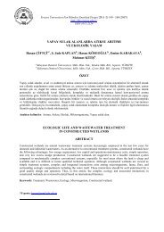
137Erciyes Üniversitesi Fen Bilimleri Enstitüsü Dergisi 26(2): 131-142 (2010)Table 1. Comparing the solutions and error analysis which has been found for N = 8, 10 at Example 4.Present method: Laguerre Methodi x iExact SolutionN = 8N = 103xy( x i ) = e y ( x i )E ( x i ) y ( x i )E ( x i )0 0 1 1 0 1 01 0.1 1.3498588076 1.3498588075 5.5 E-11 1.3498588076 6.5 E-142 0.2 1.8221188004 1.8221187709 2.9 E-08 1.8221188003 8.5 E-113 0.3 2.4596031112 2.4596019391 1.1 E-06 2.4596031028 8.3 E-094 0.4 3.3201169227 3.3201007911 1.6 E-05 3.3201167163 2.0 E-075 0.5 4.4816890703 4.4815647656 1.2 E-04 4.4816865957 2.4 E-066 0.6 6.0496474644 6.048983534 6.6 E-04 6.0496285489 1.8 E-057 0.7 8.1661699126 8.1634153481 2.7 E-03 8.1660638118 1.0 E-048 0.8 11.023176381 11.013674403 9.5 E-03 11.022701699 4.7 E-049 0.9 14.879731725 14.851256761 2.8 E-02 14.877944531 1.7 E-031 1 20.085536923 20.00915 7.6 E-02 20. 079663 5.8 E-038.00E-027.00E-02E (x )6.00E-025.00E-024.00E-023.00E-022.00E-021.00E-020.00E+000 0.1 0.2 0.3 0.4 0.5 0.6 0.7 0.8 0.9 1xN=8 N=10Figure 1. Numerical results of Example 4 for N = 8, 10 .

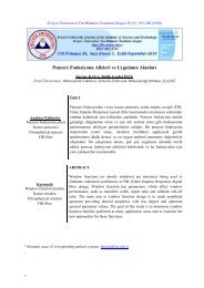
138Erciyes Üniversitesi Fen Bilimleri Enstitüsü Dergisi 26(2): 131-142 (2010)Example 5. Consider the following the integral equation in [4]12x+352x−t31y( x)= e − ∫ e y(t)dt .3We give numerical analysis for various N values in Table 2 and Figure 2, 3.108765y(x)432100 0,1 0,2 0,3 0,4 0,5 0,6 0,7 0,8 0,9 1xExact Solution BPF-Method TF-Method Laguerre Method(N=11)Figure 2. Comparing the solutions with the other methods which has been found for N = 11at Example5.7,00E-036,00E-035,00E-03E(x)4,00E-033,00E-032,00E-031,00E-030,00E+000 0,1 0,2 0,3 0,4 0,5 0,6 0,7 0,8 0,9 1xN=7 N=9 N=11Figure 3. Numerical results of Example 5 for N = 7,9, 11.

139Erciyes Üniversitesi Fen Bilimleri Enstitüsü Dergisi 26(2): 131-142 (2010)Table 2. Error analysis of Example 5 for the x values and comparison of present method, exact and themethods in [4] ( N = 7,9,11).ix iExact Solution2xy( x i ) = ePresent method : Laguerre MethodN = 7N = 9N = 11y ( x i ) E ( x i ) y ( x i ) E ( x i ) y ( x i ) E ( x i )0 0 1 1. 00025 2.5 E-05 1. 00001 1.0 E-05 1 01 0.1 1.22140 1. 22171 3. 0 E-04 1. 22141 1. 1 E-05 1. 2214 3. 2 E-082 0.2 1.49182 1. 49220 3. 7 E-04 1. 49184 1. 2 E-05 1. 49182 2. 6 E-073 0.3 1.82212 1. 82257 4. 5 E-04 1. 82213 1. 4 E-05 1. 82212 8. 6 E-074 0.4 2.22554 2. 22609 5. 5 E-04 2. 22556 1. 6 E-05 2. 22554 2. 0 E-065 0.5 2.71828 2. 71893 6. 5 E-04 2. 7183 1. 8 E-05 2. 71828 3. 8 E-066 0.6 3.32012 3. 32083 7. 0 E-04 3. 32014 1. 9 E-05 3. 32011 6. 5 E-067 0.7 4.05520 4. 05578 5. 8 E-04 4. 05522 1. 6 E-05 4. 05519 1. 0 E-058 0.8 4.95303 4. 95298 4. 9 E-05 4. 95303 4. 8 E-06 4. 95302 1. 5 E-059 0.9 6.04965 6. 04777 1. 8 E-03 6. 04957 8. 0 E-05 6. 04962 2. 2 E-0510 1 7.38906 7. 3828 6. 2 E-03 7. 38876 2. 9 E-04 7. 38902 3. 6 E-05ix iBPF Method in [4](Block Pulse Fnc.)m = 32TF Method in [4](Triangular Fnc.)0 0 1.031832 0.9998441 0.1 1.244627 1.2215982 0.2 1.501307 1.4922943 0.3 1.810922 1.8226844 0.4 2.184388 2.2258805 0.5 2.804810 2.7178576 0.6 3.383247 3.3206487 0.7 4.080975 4.0564748 0.8 4.922595 4.9545709 0.9 5.937783 6.05056810 1 7.162334 7.387901

140Erciyes Üniversitesi Fen Bilimleri Enstitüsü Dergisi 26(2): 131-142 (2010)Example 6. Our last example is the equationy12x−2t( x)= e − x + ( xe ) y(t)dtThe comparison of solutions (for N = 7, 9, 11) with exact solution∫0.xe 2 is given in Table 3 and Fig. 4.ix iExactSolution2y( x i ) = eTable 3. Error analysis of Example 6 for the x values.xPresent method: Laguerre MethodN = 7 y x ) N = 9 y x )N = 11 y x )( i0 0 1 1 1 11 0.1 1.221402758 1. 220964379 39 1. 22138590267 1. 221402725192 0.2 1.491824698 1. 490947923 22 1. 49179098664 1. 491824437383 0.3 1.8221188 1. 820803218 17 1. 82206823216 1. 822117935604 0.4 2.225540928 2. 223782850 89 2. 22547347465 2. 225538915205 0.5 2.718281828 2. 716062074 73 2. 71819724813 2. 718277975046 0.6 3.320116923 3. 317363876 34 3. 32001387690 3. 320110403087 0.7 4.055199967 4. 051699242 40 4. 05507286033 4. 055189787348 0.8 4.953032424 4. 948235426 23 4. 95286220449 4. 953017206509 0.9 6.049647464 6. 042305014 51 6. 04937847363 6. 0496246489510 1 7.389056099 7. 376568593 90 7. 38854396716 7. 38901959700i x i N = 7 E ( x i ) N = 9 E ( x i ) N = 11 E ( x i )0 0 0 0 01 0.1 4. 3 E-04 1. 6 E-05 3. 2 E-082 0.2 8. 7 E-04 3. 3 E-05 2. 6 E-073 0.3 1. 3 E-03 5. 0 E-05 8. 6 E-074 0.4 1. 7 E-03 6. 7 E-05 2. 0 E-065 0.5 2. 2 E-03 8. 4 E-05 3. 8 E-066 0.6 2. 7 E-03 1. 0 E-04 6. 5 E-067 0.7 3. 5 E-03 1. 2 E-04 1. 0 E-058 0.8 4. 7 E-03 1. 7 E-04 1. 5 E-059 0.9 7. 3 E-03 2. 6 E-04 2. 2 E-0510 1 1. 2 E02 5. 1 E-04 3. 6 E-05( i( i

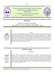
141Erciyes Üniversitesi Fen Bilimleri Enstitüsü Dergisi 26(2): 131-142 (2010)E (x )1,40E-021,20E-021,00E-028,00E-036,00E-034,00E-032,00E-030,00E+000 0,1 0,2 0,3 0,4 0,5 0,6 0,7 0,8 0,9 1xN=7 N=9 N=11Figure 4. Numerical results of Example 6 for N = 7,9, 11 .5. CONCLUSIONS AND DISCUSSIONSIn this paper, the usefulness of the methodpresented for the approximate solution ofFredholm integral equation (1) is demonstrated.To show the accuracy of the method, fiveintegral equations are chosen. A considerableadvantage of the method is that the solution isexpressed as a truncated Laguerre series. Thismeans that, after calculation of the Laguerrecoefficients, the solution y (x)can be easilyevaluated for arbitrary values of x at lowcomputation effort. If the functions f (x)andK ( x,t)can be expanded to the Laguerre seriesin a ≤ x, t ≤ b , then there exists the solutiony (x) ; otherwise, the method cannot be used in.On the other hand, it would appear that ourmethod shows to best advantage when theknown functions f (x)and K ( x,t)haveTaylor series about the origin which convergerapidly. To get the best approximating solutionof the equation, we must take more terms fromthe Laguerre expansions of functions, especiallywhen they converge slowly. Briefly, forcomputational efficiency, the truncation limitN must be chosen sufficiently large.REFERENCES1. L. Fox, I. Parker, Chebyshev polynomials inNumerical Analysis, Clarendon Press,Oxford, 1968.2. N. K. Basu, SIAM J. Numer. Anal., 10, 496-505, 1973.3. Arfken,G., Laguerre Functions,Mathematical Methods for Physicists,1985.4. E. Babolian, H.R. Marzban, M. Salmani,Using triangular orthogonal functions forsolving Fredholm integral equations of thesecond kind, App. Math. and Comput., 201,452-464, 2008.5. R. Farnoosh, M. Ebrahimi, Monte Carlomethod for solving Fredholm integralequations of the second kind, App. Math.and Comput., 195, 309-315, 2008.

142Erciyes Üniversitesi Fen Bilimleri Enstitüsü Dergisi 26(2): 131-142 (2010)6. R. P. Kanwal, and K. C. Liu, A Taylorexpansion approach for solving integralequations, Int. J. Math. Educ. Sci. Technol.,20, 411-414, 1989.7. M. Sezer, S. Dogan, Chebyshev seriessolutions of Fredholm integral equations,Int. J. Math. Educ. Sci. Technol., 27, 5, 649-657, 1996.8. K. Maleknejad, M. Karami, Using the WPGmethod for solving integral equations of thesecond kind, App. Math. and Comput., 166,123-130, 2005.9. S. Yalçınbaş, M. Aynigül, T. Akkaya,Legendre Series Solutions of FredholmIntegral Equations, Math. and Comput. App.15, 3, 371-381, 2010.