ASAC 2002 Austin R. Redlack Winnipeg, Manitoba Faculty of ...

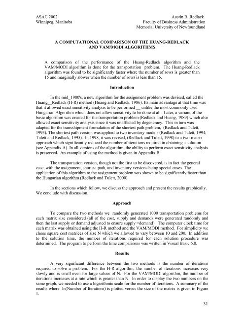
ASAC 2002Winnipeg, ManitobaAustin R. RedlackFaculty of Business AdministrationMemorial University of NewfoundlandA COMPUTATIONAL COMPARISON OF THE HUANG-REDLACKAND VAM/MODI ALGORITHMSA comparison of the performance of the Huang-Redlack algorithm and theVAM/MODI algorithm is done for the transportation problem. The Huang-Redlackalgorithm was found to be significantly faster where the number of rows is greater than15 and marginally slower when the number of rows is less than 15.IntroductionIn the mid_1980's, a new algorithm for the assignment problem was devised, called theHuang__Redlack (H-R) method (Huang and Redlack, 1986). Its main advantage at that time wasthat it allowed exact sensitivity analysis to be performed __ unlike the most commonly usedHungarian Algorithm which does not allow sensitivity to be done at all. Later, a variant of thebasic algorithm was created for the transportation problem (Redlack and Huang, 1989) which alsoallowed exact sensitivity analysis since it was unaffected by degeneracy. This in turn wasadapted for the transshipment formulation of the shortest path problem, (Redlack and Tulett,1993). The shortest path version was applied to two inventory models (Redlack and Tulett, 1994;Tulett and Redlack, 1995). In 1998, it was revised, (Redlack and Tulett, 1998) to a two-matrixapproach which significantly reduced the number of iterations required in obtaining a solution(see Appendix A). In all versions of the algorithm, the ability to perform exact sensitivity analysisis preserved. An example of using the method is given in Appendix B.The transportation version, though not the first to be discovered, is in fact the generalcase, with the assignment, shortest path, and inventory versions being special cases. Theapplication of this algorithm to the assignment problem was shown to be significantly faster thanthe Hungarian algorithm (Redlack and Tulett, 2000).In the sections which follow, we discuss the approach and present the results graphically.We conclude with discussion.ApproachTo compare the two methods we randomly generated 1000 transportation problems foreach matrix size considered (all of the cost, supply and demands were generated randomly andthen the last supply or demand adjusted to ensure supply =demand). The computer clock time foreach matrix was obtained using the H-R method and the VAM/MODI method. For simplicity wechose square cost matrices of size N which we allowed to vary between 10 and 200. In additionto the solution time, the number of iterations required for each solution procedure wasdetermined. The program to perform the time comparisons was written in Visual Basic 6.0.ResultsA very significant difference between the two methods is the number of iterationsrequired to solve a problem. For the H-R algorithm, the number of iterations increases veryslowly and is small even for large values of N. For the VAM/MODI algorithm, the number ofiterations increases at a rate which is greater than N. In order to display the two numbers on thesame graph, we needed to use a logarithmic scale for the number of iterations. A summary of theresults where ln(Number of Iterations) is plotted versus the size of the matrix is given in Figure1.31

Number of Iterationsln(Iterations)765432H-RMODI110 30 50 70 90 110 130 150 170 190Matrix SizeThe H-R method is also superior in terms of the time it takes to obtain a solution. Eachiteration involves more time than the VAM/MODI approach, but since there are significantlyfewer iterations, the actual solution time may be considerably less. The performances of the twoalgorithms are given in Figure 2200Time Trials150Time10050H-RMODI010 40 70 100 130 160 190Matrix Size32

In order to determine the order of the two solution procedures, we did a regression of ln(Numberof Iterations) versus ln(N). The results for N values in the range 50 to 200 are in the followingtable:H&RVAM/MODIIntercept -11.14 -12.19Std Error of Estimate 0.017 0.018R Squared 0.99982 0.99986N of Observations 16 16Degrees of Freedom 15 15Slope 2.882 3.296Std Err of Coef. 0.010 0.011In both cases the relationship is very linear with the order of N being roughly three.However, the VAM/MODI is on the high side of three whereas the H&R is on the low side ofthree with the difference of 0.4 being very significant. The intersection of the two lines is atln(N) approximately equal to 2.5 or N approximately equal to 12. The actual intersection of thetwo lines is N approximately equal to 15.DiscussionThe H-R method is superior to the VAM/MODI method for almost all values of N. Notonly does it allow for exact sensitivity analysis, as previous research has shown, it has now beenshown that it is also significantly faster in most cases.Thus there is now available an algorithm which will solve the assignment problem,transportation problem, shortest route problem and longest route problem either faster or onlyslightly worse than the specialized algorithms for the problems.While there is benefit in showing many different solution algorithms, there is also greatbenefit in having one algorithm which will allow concentration on formulating problems ratherthan on the learning of different solution procedures.AcknowledgmentsThe author expresses very great appreciation to Mehran Hojati for supplying a beautifulpiece of computer coding for solving the MODI method. As well as allowing the author to solvethe MODI problem, it also overcame a problem with the coding of the H&R method when thereis a number of alternate solutions..ReferencesHouthakker, H.S. ``In the Numerical Solution of the Transportation Problem,''Research, Vol. 3, 1955, 210_214.OperationsHuang, C.C., and Redlack, A.R. ``The Assignment Problem – A New Look at an Old Problem,''Proceedings of the 1986 Annual Conference Management Science Division, Vol. 7, No. 2, SureshK. Goyal (ed.), Administrative Sciences Association of Canada, 1986, 25_34.

Redlack, A.R., and Huang, C.C. ``The Transportation Problem – a Large Assignment Problem,''Proceedings of the 1989 Annual Conference. Management Science Division, Vol. 10, No. 2, UmaKumar (ed.), Administrative Sciences Association of Canada, 1989, 1_8.Redlack, A.R., and Tulett, D.M. ``Sensitivity Analysis for the Shortest Path Problem,''Proceedings of the 1993 Annual Conference. Management Science Division, Vol. 14, No. 2,Mehran Hojati (ed.), Administrative Sciences Association of Canada, 1993, 114_123.Redlack, A.R., and Tulett, D.M. ``Sensitivity Analysis for Inventory with Time VaryingDemand,'' Proceedings of the 1994 Annual Conference. Management Science Division, Vol. 15,No. 2, Jean_Marc Martel and Belaid Aouni (ed.), Administrative Sciences Association of Canada,1994, 79_88.Tulett, D.M., and Redlack, A.R. ``Parametric Analysis for Inventory with Time Varying andBack_logged Demand,'' Proceedings of the 1995 Annual Conference Management ScienceDivision, Vol. 16, No. 2, Chanchal Singh (ed.), Administrative Sciences Association of Canada,1995, 116_125.Redlack, A.R., and Tulett, D.M. ``The Transportation Algorithm - a Two Matrix Approach,''Proceedings of the 1998 Annual Conference. Management Science Division, Vol. 18, No. 2,Sajjad Zahir (ed.), Administrative Sciences Association of Canada, 1998,108-117.Redlack, A.R., and Tulett, D.M. ``A Computational Comparison of the Huang-Redlack andHungarian Algorithms”, Presented 2000 Annual Conference. Management Science Division34

Appendix A: Huang_Redlack Transportation Algorithm(1) Row Reduction 1For each row, subtract the minimum value in that row from each number in that row.(2) Column ReductionFor each column, subtract the minimum value in that column from each number in that column.(3) Make the Allocation(a) Beginning with row 1, find the first row which contains only one zero. Allocate the maximumnumber of units which can be allocated to that route and reduce the associated supply and demandrequirements by this amount. Indicate the allocation by boxing 9 the zero. If the associateddemand is nil, then cross out (using the symbol ι) any zeros in the associated column (makingthem unavailable when considering other rows). Repeat this procedure until each zero is eitherallocated or crossed out, or until each remaining row has at least two available zeros.(b) If available zeros remain, then find the columns which contain only one zero. For each ofthese, determine the allocation which could be made, and then make the largest possibleallocation. 2 Reduce the associated supply and demand requirements by this amount. If theassociated supply/demand remaining is nil, then cross out all the remaining zeros in therow/column. Return to sub_step a if any row now has only one available zero in it.(c) Continue sub_steps (a) and (b) until all zeros have been allocated or crossed out, or until norow or column has exactly one available zero.(d) If there are still at least two available zeros in some of the rows and columns, this means thatthere are alternate solutions. Find the zero to which the greatest allocation can be made, and thenmake this allocation. Reduce and cross out as in sub_step b.(e) Continue sub_steps (a) to (d) until all zeros have been either boxed or crossed out.(f) If all the supplies have been assigned, then the optimal allocations have been found; otherwisego to step 4.a.(4) Intermediate Matrix(a) Perform Procedure 1(b) If all the rows and columns are lined then there is a better solution, go to step 3.a.(c) Copy the rows lined by Procedure 1 to a new matrix and line the the columns lined byProcedure 1.(d) Find the smallest unlined cost in the new second matrix, c min . Using the column(s) associatedwith the value of c min just determined, perform Procedure 2.(e) Draw the column lines produced by Procedure 2 on the new matrix. If any new rows havebeen lined, then add c min to all the values in the rows lined by Procedure 2 and copy them to the1 The order in which the row and column reductions is done is arbitrary.2 In the case of ties, choose the route which is more to the left.35

new matrix. If all the rows have been copied over, then go to step 2. Otherwise, go to sub_step4.d.(5) Procedure 1(a) Draw a horizontal line through each row with an unallocated supply.(b) Draw a vertical line through each column which has a zero cost with a horizontal line throughit.(c) Draw a horizontal line through each row which has a vertical line through an allocated route.(d) Continue sub_steps b and c until no further lines can be drawn.(6) Procedure 2(a) Draw a vertical line through the specified column(s).(b) Draw a horizontal line through each row which has a vertical line through an allocated route.(c) Draw a vertical line through each column which has a horizontal line through a zero cost.(d) Continue sub_steps b, and c until no further lines can be drawn.36

Appendix B: An ExampleTo illustrate the algorithm, we will use the Example of Houthakker (1955). The shaded regionswill represent the cost matrix.V W X Y ZA 73 40 9 79 20 8 64 31 0 70 11B 62 93 96 8 13 7 54 85 88 0 5C 96 65 80 50 65 9 46 15 30 0 15D 57 58 29 12 87 3 45 46 17 0 75E 56 23 87 18 12 5 44 11 75 6 06 8 19 4 4To obtain the second matrix we just subtracted the minimum value in each row. Subtracting theminimum value in each column an performing the allocations we have2 a2 c 3 a1 d 2 dLine2 2 3 1 2Added20 20 08 170 11 0 3 b 37 37 17 87 28 310 74 88 04 2531 a 10 74 8805 12 4 3001591 b 2 4 30015 11 35 1705 30750 75 6 01 0 2 0 0301 c 1 1 35 17 2 075 12 b 1 1 76 7 1 2The left of the above table is the transportation tableau with the allocations in bold with the subscriptindicating the order in which the allocation was made. The unbolded numbers with subscripts indicate thesets of lines which are drawn in each of the three iterations. I would strongly recommend drawing in thelines in the order indicated in order to more easily follow the procedure. The added column indicates theorder in which the rows are copied to the second matrix. Note that 1 is added to the line numbered 2 and17 to the line numbered 3. The bold values with subscripts on the right are the minimum unlined valueswith the subscript indicating the order win which they are found. All of the rows are copied over so wesubtract the minimum value from each column and start over.37

2a 3a 2c 1c 2d Line 2 3 2 1 2 Added36 36 08 19 73 71 04 21 3 1303 4034 005 387 27004147459 7 03 3 2 0 4039002d 37 37 1 88 28 21a 9 73 7104 11b 1 1 3 2 13014 12f 1 35 1175 23b 3 3 62 10 3 3In this case we have added 1 to line numbered 2 and 3 to the line numbered 3. Subtracting theminimum value in each column and performing the assignment we have2e 2c 2g 1b 2a Line 2 2 2 1 2 Added36 34 08 19 70 70 04 2002 603 7207 51232 001 488 25111172030061 10 04 3 01 0 2 0 02h 37 35 1 89 26 21a 9 70 70 0 1 1 12d 1 1 13 1 12 22f 1 33 1273 22b 3 1 62 11 1 238

Subtracting the minimum value from each row and performing the assignment, we have 336 34 08 189 2508 69 69 04 203 3 005 604 712 1 11001 532 02 42 7202 04 861 11 01 9 00 0 0 0 0Since there are no more units to allocate, we have the optimal solution.3 In this case it would have been simpler just to subtract 1 from row 2 and add 1 to column 4.39