An elementary introduction to large deviations

• Large Deviations in Queuing Networks: Effective Bandwidths• Bypassing Modelling: Estimating the Scaled CGF2

for each positive number ǫ. This shows that the Weak Law of Large Numbersis a consequence of the Large Deviation Principle.9

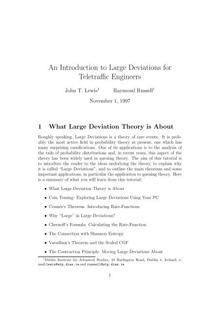
3 Cramér’s Theorem: Introducing Rate-FunctionsHarald Cramér was a Swedish mathematician who served as a consultantactuary for an insurance company; this led him to discover the first resultin Large Deviation theory. The Central Limit Theorem gives informationabout the behaviour of a probability distribution near its mean while therisk theory of insurance is concerned with rare events out on the tail of aprobability distribution. Cramér was looking for a refinement of the CentralLimit Theorem; what he proved was this:Cramér’s Theorem Let X 1 , X 2 , X 3 , . . . be a sequence of bounded, independentand identically distributed random variables each with mean m, and letM n = 1 n (X 1 + . . . + X n )denote the empirical mean; then the tails of the probability distribution of M ndecay exponentially with increasing n at a rate given by a convex rate-functionI(x):P( M n > x ) ≍ e −nI(x) for x > m,P( M n < x ) ≍ e −nI(x) for x < m.Historically, Cramér used complex variable methods to prove his theoremand gave I(x) as a power-series; later in this section we will explain why thisis a natural approach to the problem. However, there is another approachwhich has the advantage that it can be generalised in several directions andwhich has proved to be of great value in the development of the theory.We illustrate this approach in Appendix B by sketching a proof of Cramér’sTheorem which uses it; but first let us see how the theorem can be used inrisk-theory.An Application to Risk-TheoryLarge Deviation theory has been applied to sophisticated models in risk theory;to get a flavour of how this is done, consider the following simple model.Assume that an insurance company settles a fixed number of claims in afixed period of time, say one a day; assume also that it receives a steadyincome from premium payments, say an amount p each day. The sizes of theclaims are random and there is therefore the risk that, at the end of someplanning period of length T, the total amount paid in settlement of claimswill exceed the total income from premium payments over the period. Thisrisk is inevitable, but the company will want to ensure that it is small (in the10

interest of its shareholders, or because it is required by its reinsurers or someregulatory agency). So we are interested in the small probabilities concerningthe sum of a large number of random variables: this problem lies squarely inthe scope of Large Deviations.If the sizes X t of claims are independent and identically distributed, thenwe can apply Cramér’s Theorem to approximate the probability of ruin, theprobability that the amount ∑ Tt=1 X t paid out during the planning period Texceeds the premium income pT received in that period:( T∑)P X t > pT ≍ e −TI(p) .t=1So, if we require that the risk of ruin be small, say e −r for some large positivenumber r, then we can use the rate-function I to choose an appropriate valueof p:P(1T)T∑X t > pt=1≈e −re −TI(p) ≈ e −rI(p) ≈Since I(x) is convex, it is monotonically increasing for x greater than themean of X t and so the equationI(p) = r/Thas a unique solution for p.Of course, to solve this equation, we must know what I(x) is and thatmeans knowing the statistics of the sizes of the claims. For example, if thesize of each claim is normally distributed with mean m and variance σ 2 , thenthe rate-function isI(x) = 1 ( ) 2 x − m.2 σIt is easy to find the solution to the equation for p in this case: it is p =m + σ √ 2r/T; thus the premium should be set so that the daily incomeis the mean claim size plus an additional amount to cover the risk. Theratio (p − m)/m is called the safety loading; in this case, it is given by(σ/m) √ 2r/T. Notice that σ/m is a measure of the size of the fluctuationsin claim-size, while √ T/2r is fixed by the regulator.r/T11

Why “Large” in Large Deviations?Recall what the Central Limit Theorem tells us: if X 1 , X 2 , X 3 , . . . is a sequenceof independent and identically distributed random variables withmean µ and variance σ 2 < ∞, then the average of the first n of them,M n = 1 (X n 1 + . . . + X n ) is approximately normal with mean µ and varianceσ 2 /n. That is, its probability density function is1f(x) = √ n (x−µ) 22πσ2 /n e− 2 σ 2 ,and the approximation is only valid for x within about σ/ √ n of µ. If weignore the prefactor in f and compare the exponential term with the approximationthat Cramér’s Theorem gives us, we see that the terms (x −µ) 2 /2σ 2occupy a position analogous to that of the rate function. Let us look againat the coin tossing experiments: for x close to 1/2, we can expand our ratefunctionin a Taylor series:x ln x + (1 − x) ln(1 − x) + ln 2 = (x − 1 2 )22 × 1 + . . .4The mean of each toss of a coin is 1/2, and the variance of each toss is 1/4;thus the rate-function for coin tossing gives us the Central Limit Theorem. Ingeneral, whenever the rate-function can be approximated near its maximumby a quadratic form, we can expect the Central Limit Theorem to hold.So much for the similarities between the CLT and Large Deviations; thename “Large Deviations” arises from the contrast between them. The CLTgoverns random fluctuations only near the mean – deviations from the meanof the order of σ/ √ n. Fluctuations which are of the order of σ are, relative totypical fluctuations, much bigger: they are large deviations from the mean.They happen only rarely, and so Large Deviation theory is often describedas the theory of rare events – events which take place away from the mean,out in the tails of the distribution; thus Large Deviation theory can also bedescribed as a theory which studies the tails of distributions.Chernoff’s Formula: Calculating the Rate-FunctionOne way of calculating the rate-function for coin-tossing is to apply Stirling’sFormula in conjunction with the combinatorial arguments we used earlier;this is sketched in Appendix A. There is, however, an easier and moregeneral method for calculating the rate-function for the independent case; itis known as Chernoff’s Formula. To understand the idea behind it, we lookat a way of getting an upper bound on a tail probability which is often usedin probability theory.12

3Exponential functionIndicator function210aFigure 6: I (a,∞) x ≤ e θx /e θa for each a and each θ > 0.Chernoff’s BoundFirst let us look at a simple bound on P( M n > a ) known as Chernoff’sbound. We rewrite P( M n > a ) as an expectation using indicator functions.The indicator function of a set A ⊂ R is the function I A· defined by{ 1 if x ∈ A,I A x :=0 otherwise.Figure 6 shows graphically that, for each number a and each positive numberθ, I (a,∞) x ≤ e θx /e θa . Now note that E I (na,∞) nM n = P( nM n > na ) and soP( M n > a ) = P( nM n > na )= E I (na,∞) nM n≤ E e θnMn /e θna13

= e −θna E e θ(X 1+...+X n)= e −θna ( E e θX i) n;we take this last step 1 the X i ’s are independent and identically distributed.By defining λ(θ) = ln Ee θX 1we can write P( M n > a ) ≤ e −n{θa−λ(θ)} ; sincethis holds for each θ positive, we can optimise over θ to getP( M n > a ) ≤ minθ>0 e−n{θa−λ(θ)} = e −nmax θ>0{θa−λ(θ)} .If a is greater than the mean m, we can obtain a lower bound which givesP( M n > a ) ≍ e −nmax θ{θa−λ(θ)} ;This is just a statement of the Large Deviation principle for M n , and is thebasis forChernoff’s Formula: the rate-function can be calculated from λ, the cumulantgenerating function:I(x) = max{xθ − λ(θ)},θwhere λ is defined byλ(θ) := lnEe θX j.Coin-Tossing RevisitedWe explored the large-deviations of the coin-tossing experiment with a faircoin in some detail and painstakingly built up a picture of the rate-functionfrom the asymptotic slopes of our log-probability plots. We could do thesame again for a biased coin, but Cramér’s Theorem tells us immediatelythat we will again have a Large Deviation principle. Since the outcomes ofthe tosses are still bounded (either 0 or 1) and independent and identicallydistributed, Cramér’s Theorem applies and we can calculate the rate-functionusing Chernoff’s Formula: let p be the probability of getting heads, so thatthe cumulant generating function λ isλ(θ) = ln Ee θX 1= ln(pe θ + 1 − p).By Chernoff’s Formula, the rate-function is given byI(x) = max {xθ − λ(θ)} .θ14

1.6Asymptotic decay-rate of tail1.41.210.80.60.40.200 0.2 0.4 0.6 0.8 1Point at which tail startsFigure 7: The rate-function for coin tossing with a biased coin (p=0.2).Exercise 5 Use differential calculus to show that the value of θ which maximisesthe expression on the right-hand side is θ x = lnx/p −ln(1 −x)/(1 −p)and hence that the rate-function isI(x) = x ln x p+ (1 − x) ln1 − x1 − p .Figure 7 shows a plot of I(x) against x for p = 0.25.Why Does Chernoff’s Formula Work?The cumulants of a distribution are closely related to the moments. Thefirst cumulant is simply the mean, the first moment; the second cumulantis the variance, the second moment less the square of the first moment.15

The relationship between the higher cumulants and the moments is morecomplicated, but in general the k th cumulant can be written in terms of thefirst k moments. The relationship between the moments and the cumulantsis more clearly seen from their respective generating functions. The functionφ(θ) = Ee θX 1is the moment generating function for the X’s: the k th momentof the X’s is the k th derivative of φ evaluated at θ = 0:d kdθ kφ(θ) = EXk 1e θX 1∣d k φ ∣∣∣θ=0= E X kdθ k 1 = k th momentThe cumulant generating function (CGF) is defined to be the logarithm ofthe moment generating function, λ(t) := ln φ(t), and the cumulants are thenjust the derivatives of λ:ddθ λ(θ) ∣∣∣∣θ=0= m,d 2dθ 2λ(θ) ∣∣∣∣θ=0= σ 2 , ...So, why does Chernoff’s Formula work? In order to calculate the CentralLimit Theorem approximation for the distribution for M n , we must calculatethe mean and variance of the X’s: essentially we use the first two cumulantsto get the first two terms in a Taylor expansion of the rate-function to giveus a quadratic approximation. It is easy to see that, if we want to get the fullfunctional form of the rate-function, we must use all the terms in a Taylorseries — in other words, we must use all the cumulants. The CGF packagesall the cumulants together, and Chernoff’s Formula shows us how to extractthe rate-function from it.Proving Cramér’s TheoremCramér’s proof of his theorem was based essentially on an argument usingmoment generating functions and gave the rate-function as a power series.After seeing the connection with the Central Limit Theorem and Chernoff’sFormula, we can see how this is a natural approach to take; indeed, one ofthe standard proofs of the Central Limit Theorem is based on the momentgenerating function. This method of proof has the drawback that it is noteasy to see how to adapt it to more general situations. There is a more elegantargument which establishes the theorem and which can easily be modified toapply to random variables which are vector-valued and to random variables16

which are not necessarily independent. This argument shows at the sametime that the rate-function is convex; we sketch this proof in appendix B.17

4 The Connection with Shannon EntropyWe are often asked “How does Shannon entropy fit into Large Deviationtheory?” To answer this question fully would sidetrack us into an expositionof the ideas involved in Information Theory. However, we will use Cramér’sTheorem to give a proof of the Asymptotic Equipartition Property, one ofthe basic results of Information Theory; in the course of this, we will see howShannon entropy emerges from a Large Deviation rate-function.Let A = {a 1 , . . .a r } be a finite alphabet. We describe a language writtenusing this alphabet by assigning probabilities to each of the letters; theserepresent the relative frequency of occurrence of the letters in texts writtenin the language. We write p k for the relative frequency of the letter a k . Asa first approximation, we ignore correlations between letters and take theprobability of a text to be the product of the probabilities of each of thecomponent letters. This corresponds to the assumption that the sequenceof letters in any text is an independent and identically distributed sequenceof random letters. Let Ω n be the set of all texts containing exactly n letters;then the probability of the text ω = (ω 1 , ω 2 , . . .ω n ) (where each of theω i ’s represents a letter) is just p n 11 p n 22 . . .p nrr , where n k is the number of occurrencesof the letter a k in the text ω. We write α[ω] = p n 11 pn 22 . . .pnr r toexplicitly denote the dependence of this probability on the text.Claude Shannon made a remarkable discovery: if some letters are moreprobable (occur more frequently), then there is a subset Γ n of Ω n consistingof “typical texts” with the following properties:• texts not in Γ n occur very rarely, so that α[Γ n ] = ∑ ω∈Γ nα[ω] is closeto 1;• for n large, Γ n is much smaller than Ω n :#Γ n#Ω n≍ e −nδ for some δ > 0;• all texts in Γ n have roughly the same probability.This result is known as the Asymptotic Equipartition Property (AEP). Shannonintroduced a quantity which measures the non-uniformity of a probabilitymeasure; it is known as the Shannon entropy. The Shannon entropy isdefined byh(α) := −p 1 ln p 1 − p 2 ln p 2 . . . − p r ln p r .We see that 0 ≤ h(α) ≤ lnr; the maximum value lnr occurs when all thep k are equal. Because of the applications of information theory to computer18

Exercise 6 Use differential calculus to show that t must satisfy∂λ∂t k=p k e t kp 1 e t 1 + . . . + pr e tr = µ[{a k}],and sot k = ln µ[{a k}]+ λ(t).p kSubstitute this into the expression to be minimised to show thatwhere m k = µ[{a k }].I(µ) = m 1 ln m 1p 1+ . . . + m r ln m rp r,The expression m 1 lnm 1 /p 1 + . . . + m r ln m r /p r is written more simply asD(µ‖α) and is known as the informational divergence.Let us look again at the statement of Cramér’s Theorem: we see thatthe distribution of M n is concentrated near the mean m, the place where therate-function vanishes.Exercise 7 Show that it follows from Cramér’s Theorem that, as n increases,limn→∞ P( m − δ < M n < m + δ ) = 1,for any δ > 0.In Sanov’s Theorem, the rate-function is D(µ‖α); this vanishes if and onlyif µ = α. So we have thatlim α[L n ≈ α] = 1,n→∞and it follows that, if we choose Γ n to be those texts in which the relativefrequencies of the letters are close to those specified by α, then α[Γ n ] willconverge to 1 as n increases. Thus Γ n consists of the most probable texts andtexts which are not in Γ n occur only very rarely. To estimate the size of Γ n ,we apply Sanov’s Theorem a second time. Let β be the uniform probabilitymeasure which assigns probability 1/r to each of the r letters in A; thenβ[Γ n ] = #Γ n /#Ω n . Now, Γ n is the set of texts ω for which L n (ω) is closeto α, and so we can apply Sanov’s Theorem to the distribution of L n withrespect to β:β[Γ n ] = β[L n ≈ α] ≍ e −nD(α‖β) .20

ButD(α‖β) = p 1 (lnp 1 − ln 1/r) + . . . + p r (ln p r − ln 1/r)= ln r − h(α)= δ,and so #Γ n /#Ω n ≍ e −nδ .21

statistical thermodynamics, yields a direct proof of the existence of a ratefunctionsatisfying the requirements listed in appendix C and uses Varadhan’sTheorem to calculate it; the second is known as the Gärtner-Ellis Theorem— we will examine it after we have described the first approach.The Ruelle-Lanford ApproachWe illustrate the Ruelle-Lanford approach by outlining the proof of Cramér’sTheorem for I.I.D. random variables which is given in appendix B. We thenindicate how the argument goes when we relax the condition of independence.It is well known that if a sequence {a n } of numbers is such thata n ≥ a m whenever n > m (1)then its limit exists and is equal to its least upper bound:lim a n = sup a n (2)n→∞Let s n (x) := ln P( M n > x ); if we could prove that the sequence {s n /n}satisfies Equation 1, then the existence of the limit would follow. We can’tquite manage that. However we can use the I.I.D. properties of the randomvariables {X n } to prove thatn>0It then follows from a theorem in analysis thats m+n (x) ≥ s m (x) + s n (x) (3)s nlimn→∞ n = sup s nn>0 n .This proves the existence of the rate-function1I(x) = − limn→∞ n ln P( M n > x ).If we give names to these conditions, we can write slogans which are easyto remember. If Equation 1 holds, we say that {a n } is monotone increasing;if Equation 2 holds, we say that {a n } is approximately monotone increasing;if Equation 3 holds, we say that {s n } is super-additive. This is illustratedin Figure 8 using the coin-tossing data; the super-additive sequence{ln P( M n > 0.6 )} is shown on top, and the approximately monotone increasingsequence {ln P( M n > 0.6 )/n} is shown on the bottom converging to itsmaximum value.23

0-0.5-1ln P( Mn/n > 0.6 )-1.5-2-2.5-3-3.5-4-4.5010 20 30 40 50 60 70 80 90 100n-0.05ln P( Mn/n > 0.6 ) /n-0.1-0.15-0.2-0.25-0.3-0.35-0.410 20 30 40 50 60 70 80 90 100nFigure 8: The distribution of the mean for coin-tossing: ln P(M n > 0.6 )(top) is super-additive and so ln P( M n > 0.6 )/n (bottom) is approximatelymonotone; as n increases, ln P( M n > 0.6 )/n converges to its maximumvalue.24

ate-function I and f is a continuous function, then {f(X n )} satisfies a LargeDeviation principle with rate-function J, where J is given byJ(y) = min {I(x) : f(x) = y }.It is called the “contraction” principle because typically f is a contraction inthat it throws detail away by giving the same value f(x) to many differentvalues of x.Why does the contracted rate-function J have this form? Consider P( f(X n ) ≈ y ):there may be many values of x for which f(x) = y, say x 1 , x 2 , . . .,x m , and soP(f(X n ) ≈ y ) = P( X n ≈ x 1 or X n ≈ x 2 . . . or X n ≈ x m )= P( X n ≈ x 1 ) + P( X n ≈ x 2 ) + . . . + P( X n ≈ x m )≍ e −nI(x 1) + e −nI(x 2) + . . . + e −nI(xm) .As n grows large, the term which dominates all the others is the one forwhich I(x k ) is smallest, and soP( f(X n ) ≈ y ) ≍ e −nmin{ I(x): f(x)=y } = e −nJ(y) .To see the Contraction Principle in action, let us return to the AEP: wesaw that the empirical distribution L n [B] = (δ X1 [B]+. . .+δ Xn [B])/n satisfiesa Large Deviation principle in thatP( L n ≈ µ ) ≍ e −nI(µ)Suppose we take the letters a 1 , . . .a r to be real numbers and that, instead ofinvestigating the distribution of the empirical distribution L n , we decide toinvestigate the distribution of the empirical mean M n = a 1 n 1 /n+. . .+a r n r /n.Do we have to go and work out the Large Deviation Principle for M n fromscratch? No, because M n is a continuous function of L n ; it is a very simplefunctionM n = f(L n ) = a 1 L n [{a 1 }] + . . . + a r L n [{a r }].The contraction principle applies, allowing us to calculate the rate-functionJ for {M n } in terms of the rate-function I for {L n }. We have thatJ(x) = minµD(µ‖α) subject to a 1 m 1 + . . . + a r m r = x,where m k = µ[{a k }]. This is a simple constrained optimisation problem: wecan solve it using Lagrange multipliers.27

Exercise 9 Show that the value of µ which achieves the minimum is givenbye βa k pkµ[{a k }] =,e βa 1 p1 + . . . + e βar p rwhere β is the Lagrange multiplier whose value can be determined from theconstraint. (Hint: Note that there are two constraints on m – the requirementthat a 1 m 1 + . . . + a r m r be x and the fact that µ is a probability vector – andso you will need two Lagrange multipliers!)28

6 Large Deviations in Queuing SystemsA queuing network consists of a network through which customers flow, requiringsome kind of processing by servers at the nodes. Typically the servershave limited capacity and the customers must queue while waiting for service.The basic problems in queuing theory is to analyse the behaviour of asingle element of a network: the single-server queue.For simplicity, we will consider a single-server queue in discrete time and,ignoring any considerations of multiple classes of customers or priority, wetake the discipline to be FIFO (First In, First Out). Let us set up somenotation: let X i be the amount of work brought by customers arriving attime i, let Y i be the amount of work the server can do at time i, and let Q ibe the queue-length (i.e. the amount of work waiting to be done) at time i.The dynamics of the system are very simple: the length of the queue at time0, say, is the sum of the length of the queue at time -1 and the work whicharrives at time -1 less the work which can be done at time -1. The servicecannot be stored and so, if the service available is greater than the sum ofthe work in the queue and the work which arrives, then the new queue-lengthis not negative but zero. This can all be expressed neatly in the formulaQ 0 = max {0, X −1 − Y −1 + Q −1 },known as Lindley’s equation. We can iterate it, substituting for Q −1 ; tosimplify notation, we set Z i = X −i − Y −i for all i:Applying it again gives usQ 0 = max {0, Z 1 + Q −1 }= max {0, Z 1 + max {0, Z 2 + Q −2 }}= max {0, Z 1 , Z 1 + Z 2 + Q −2 }.Q 0 = max {0, Z 1 , Z 1 + Z 2 + max {0, Z 3 + Q −3 }}= max {0, Z 1 , Z 1 + Z 2 , Z 1 + Z 2 + Z 3 + Q −3 } .It is clear that, by defining W t = Z 1 + . . . + Z t , we can writeQ 0 = max {W 0 , W 1 , . . .W t−1 , W t + Q −t };W t is called the workload process. If we started off at some finite time −T inthe past with an empty queue, thenQ 0 = max {W 0 , W 1 , . . .W T −1 , W T } .29

ln P( Q > q )0-1-2-3-4-5-6-7-8-9-10-110 20 40 60 80q100 120 140Figure 9: The logarithm of a typical queue-length distribution31

We can get a feeling for why this is true from the following crude argument(a proof is given in Appendix E); first notice that( )P( Q > q ) = P max W t > qt≥0= P( ∪ t≥0 {W t > q} )≤ ∑ t≥0P( W t > q ) .Since P( W t /t > x ) ≍ e −tI(x) , we haveso thatP( W t > q ) = P( W t /t > q/t ) ≍ e −tI(q/t) I(q/t)−q= eq/tI(q) I(q/2)I(q/t)−q −q −qP( Q > q ) ≍ eq+ eq/2+ . . . + eq/t+ . . .and, just as in the discussion of the Contraction Principle, the term whichdominates when q is large is the one for which I(q/t)/(q/t) is smallest, thatis the one for which I(x)/x is a minimum:I(x)−q minxP( Q > q ) ≍ e x = e −qδ .Note that we can also characterise δ in terms of the scaled CGF:θ ≤ min I(x)/x if and only if θ ≤ I(x)/xxfor all xif and only if θx − I(x) ≤ 0 for all xthus θ ≤ δ if and only if λ(θ) ≤ 0 and soif and only if max{θx − I(x)} ≤ 0;xδ = max { θ : λ(θ) ≤ 0 }.Using the Scaled CGF for Resource AllocationBuffer DimensioningIf the queue has only a finite waiting space, then δ gives us an estimateof what that buffer-size must be in order to achieve a given probability ofoverflow. Look again at Figure 9: it is clear that, if we require the probabilityof overflow to be smaller than e −9 (a little over 10 −4 ), we need a buffer largerthan 120. We can use δ to give an estimate ˆP(b) of the probability of a bufferof size b overflowing:ˆP(b) = e −δb .32

Effective BandwidthsNote that in the case in which the service capacity is a constant, s per unittime, the workload process is W t = X −1 +. . .+X −t −st and the scaled CGFisλ(θ) =1limt→∞ t lnEeθWt1= limt→∞ t lnEeθ(X −1+...+X −t −st)= limt lnEeθ(X −1+...+X −t ) − sθ= λ A (θ) − sθt→∞1where λ A is the scaled CGF of the arrivals process. Thus, given the arrivalsscaled CGF, we can calculate δ as a function of s:δ(s) = max { θ : λ A (θ) ≤ sθ }.It may happen, as in ATM networks, that the buffer-size is fixed but thecapacity of the server can be varied; in that case, a natural question to askis “Given the arrivals process A t , what is the minimum service capacity s prequired to guarantee that the probability of buffer-overflow is less than somegiven level p?”. We can use the approximation P( Q > b ) ≈ e −δ(s)b to givean estimate of s p :s p = min { s : e −δ(s)b ≤ p } .Exercise 10 Show that s p = λ A (θ p )/θ p where θ p = (− ln p)/b.s p is, in general, larger than the mean bandwidth of the arrivals; and is knownas the effective bandwidth of the arrivals. The function λ A (θ)/θ is known asthe effective bandwidth function and the approximation P( Q > b ) ≈ e −δ(s)bis known as the effective bandwidth approximation.Effective Bandwidths in Risk TheoryRecall the simple model of risk theory we discussed in Section 3: an insurancecompany settles a fixed number of claims in a fixed period of time, say one aday, and receives a steady income from premium payments, say an amountp each day. Since the sizes of the claims are random, there is the risk that,at the end of the planning period T, the total amount paid in settlementof claims will exceed the total assets of the company. When we discussedthis model before, we assumed that the only asset the company has to cover33

If we denote by θ ∗ the value of θ which maximises this expression, then weget thatθ ∗ p + θ ∗ u/T − λ(θ ∗ ) = r/Thence, by taking p = λ(θ ∗ )/θ ∗ and u = r/θ ∗ we get a solution in which thepremium rate p is the effective bandwidth of the claims process at a value θ ∗of θ which gives a probability e −θ∗u = e −r of ruin in a buffer of size u.Bypassing Modelling: Estimating the Scaled CGFAll we need for the scaled CGF of the arrivals to exist is for the arrivals to bestationary and mixing. If these two conditions are satisfied, we can use thescaled CGF to make predictions about the behaviour of the queue. One wayto get the scaled CGF for the arrivals is to make a suitable statistical model,fit the parameters of the model to the data and then calculate the scaled CGFfrom the model. There are a number of problems with this approach. Firstly,real traffic streams cannot be accurately represented by simple models; anyrealistic model would have to be quite complex, with many parameters to befitted to the data. Secondly, the calculation of the scaled CGF for any but thesimplest model is not easy. Thirdly, even if you could find a realistic model,fit it to your data and calculate the scaled CGF, this would be a wastefulexercise: the scaled CGF is a Large Deviation object, and it does not dependon the details of the model, only on its “bulk properties”. Hence all theeffort you put into fitting your sophisticated model to the data is, to a largeextent, lost. Our approach is to ask “Why not measure directly what youare looking for?” There are many good precedents for this approach. Whenengineers design a steam turbine they need to know the thermodynamicproperties of steam. To find this out, they do not make a sophisticatedstatistical mechanical model of water and calculate the entropy from that;instead, they measure the entropy directly in a calorimetric experiment, or(more likely) they use steam tables – based on somebody else’s measurementsof the entropy. Now, we make the observation that thermodynamic entropyis nothing but a rate-function. So if you want the thermodynamics (thatis, the Large Deviations) of your queuing system, why not measure directlythe entropy (that is, the rate-function) of the workload process? How do wemeasure the rate-function – or, equivalently, the scaled CGF – of the workloadprocess? Consider the case in which the service capacity is a constant, s perunit time; the workload process is then W t = X −1 + . . . + X −t − st and thescaled CGF isλ(θ) = λ A (θ) − s35

where λ A is the scaled CGF of the arrivals process. If the arrivals X i areweakly dependent, we can approximate the scaled CGF by a finite-time cumulantgenerating function:λ A (θ) ≈ λ (T)A (θ) = 1 T lnEeθA T,for T sufficiently large. We can now estimate the value of the expectation bybreaking our data into blocks of length T and averaging over them:ˆλ A (θ) := 1 T ln 1 Kwhere the ˜X’s are the block sumsk=K∑k=1e θ ˜X k,˜X 1 := X 1 + . . . + X T , ˜X2 := X T+1 + . . . + X 2T , etc.This yields estimates of both the effective bandwidth ˆλ(θ)/θ and, giventhe value of s, the asymptotic decay-rate ˆδ of the queue-length distributionthrough}ˆδ := max{θ : ˆλ(θ) ≤ 0 .Other EstimatorsIs this the only way to estimate λ? Not at all; there are many ways toestimate it and, indeed, different methods may be appropriate for differentarrivals processes. Consider what exactly we are doing when we use theestimatorˆλ(θ) = 1 T ln 1 Kk=K∑k=1e θ ˜X k.If the ˜X k ’s are independent, then the scaled CGF of the X i ’s is just thecumulant generating function of the ˜X k ’s, and the above estimator is exactlywhat we need to measure the latter. Thus, when we say that we needed Tto be large enough for the finite time cumulant generating function λ (T) tobe a good approximation to the asymptotic one λ, we really mean that weneed T to be large enough for the block-sums ˜X k to be independent. Notonly can we easily calculate the scaled CGF for independent sequences, butwe can also do so for Markov sequences. Thus, if we use an estimator basedon a Markov structure, we only need T to be large enough that the ˜X k ’sare approximately Markov; such an estimator is tailor-made for the case ofMarkovian arrivals.36

There is a whole class of estimators, similar to the simple I.I.D. estimatorˆλ shown above, but which, instead of using one fixed size T for each block,use variable block-sizes. To see how they work, we need to consider the LargeDeviations of random time-changes.The Large Deviations of Random Time-ChangesSuppose we have a Large Deviation principle (LDP) for some process {S t },in thatP( S t ≈ s ) ≍ e −tI(s) ;if we take an increasing sequence {t n } of times such that t n → ∞, thenobviously we also have a LDP for the sequence {S tn }:P( S tn ≈ s ) ≍ e −tnI(s) ;If t n /n → τ, then we can also write P( S tn ≈ s ) ≍ e −nτI(s) . What happensif, instead of a deterministic sequence {t n }, we take a sequence of randomtimes {T n }? If {T n } satisfies the Weak Law of Large Numbers, so thatlim n P( |T n /n − τ| > ǫ ) = 0 for any positive number ǫ, then we might expectthatP( S Tn ≈ s ) ≍ e −nτI(s) .as before. What if {T n } satisfies a LDP? Obviously the Large Deviations of{T n } get mixed in with those of {S t }. We could ask a more specific question:if we have a joint LDP for S Tn and T n , so thatP( S Tn ≈ s, T n /n ≈ τ ) ≍ e −nJ(s,τ) ,then how are I(s) and J(s, τ) related?To answer that, we need to look at the joint Large Deviation principlefor S t and N t , where N t is the counting process associated with T n :N t = sup {n : T n ≤ t} ;N t is the number of random times which have occurred up to time t. A betterquestion is the following: if S t and N t satisfy a LDP jointlythen is it true thatP( S t ≈ s, N t /t ≈ ν ) ≍ e −tI(s,ν) ,P( S Tn ≈ s, T n /n ≈ τ ) ≍ e −nJ(s,τ)and, if so, what is the relationship between I(s, ν) and J(s, τ)?37

The answer is simple: yes (under appropriate hypotheses on the processesS t and N t and the rate-function I), and the relationship between the ratefunctionsisI(s, 1/τ)J(s, τ) = .τConsider the following scaled cumulant generating function1µ(θ) := limn→∞ n lnEeθTnS Tn ;an application of Varadhan’s Theorem allows us to calculate µ in terms of J:∫E e θTnS Tn= e θnτs dP(S Tn ≈ s, T n /n ≈ τ )∫≍ e θnτs e −nJ(s,τ) ds dτ≍ e n maxs,τ {θτs−J(s,τ)} .Thus µ(θ) = max s,τ {θτs − J(s, τ)} and, rewriting J in terms of I, we havethatµ(θ) = max τ{θs − I(s, 1/τ)}.s,τConsider also the scaled CGF of S t1λ(θ) = lim ln E eθtStt→∞ tExercise 11 Use Varadhan’s Theorem as we did above to show thatλ(θ) = max{θs − I(s, ν)}.s,ν(Hint: Apply Varadhan’s Theorem to E e θtSt+αNt and then set α = 0.)Is there any connection between λ and µ? Yes, they are related as follows:max{θs − I(s, ν)} ≤ 0 if and only if {θs − I(s, ν)} ≤ 0s,νfor all s and all ν > 0if and only if {θs − I(s, 1/τ)} ≤ 0 for all s and all τ > 0if and only if τ{θs − I(s, 1/τ)} ≤ 0 for all s and all τ > 0if and only if max τ{θs − I(s, 1/τ)} ≤ 0s,τand so λ(θ) ≤ 0 if and only if µ(θ) ≤ 0 and hence{θ : λ(θ) ≤ 0 } = { θ : µ(θ) ≤ 0 } .38

This means that, if the process S t is the average workload W t /t of a queueup to time t, then we can characterise the asymptotic decay rate δ of thequeue-length distribution as eitherδ = max {θ : λ(θ) ≤ 0 } or δ = max { θ : µ(θ) ≤ 0 }Let us look more closely at µ: it is defined as1limn→∞ n ln E 1eθW Tn = limn→∞ n ln E eθ(X −1+...+X −Tn −sT n) ;where s is the service rate of the queue and T n is any increasing sequence ofrandom times. This tells us that, when estimating δ, we are not restrictedto using a sequence of fixed block-sizes to aggregate the observations of thearrivals but are free to use any sequence {T n } of large block-sizes. We cantherefore choose blocks which reflect the structure of the arrivals process togive us estimators which have lower bias and/or variance.AThe Large Deviations of Coin-Tossing: ABare-Hands CalculationAnother way to see Large Deviations at work is to use Stirling’s Formulain conjunction with the combinatorial expressions for the tail-probabilities.Thus consider P( M n < a ):P( M n < a ) =⌈a⌉−1∑k=0( nk) 12 n.If a < 1/2, then each term in the sum is bounded by n C ⌈na⌉ and so( ) n 1P( M n < a ) ≤ ⌈na⌉⌈na⌉ 2 =: A n.nNow consider ln A n : we can rewrite ln n C ⌈na⌉ as− ⌈na⌉ ( ) ()1n ⌈na⌉ ln ⌈na⌉! − ln ⌈na⌉ ⌊n(1 − a)⌋ 1−n ⌊n(1 − a)⌋ ln ⌊n(1 − a)⌋! − ln ⌊n(1 − a)⌋( ) 1+n ln n! − ln nand use Stirling’s Formula− ⌈na⌉nlimn→∞ln⌈na⌉n( ) 1n ln n! − ln n = −139⌊n(1 − a)⌋ ⌊n(1 − a)⌋− lnn n

to get1limn→∞ n ln A n = −a ln a − (1 − a) ln(1 − a) − ln 2.Let us look again at P( M n < a ): not only can we bound it above bysomething which decays exponentially, but we can also bound it below bysomething which decays exponentially at the same rate. So long as a > 0,( )n 1P( M n < a ) ≥⌈na⌉ − 1 2 n.Exercise 12 Show that( )1limn→∞ n ln n 1= −a ln a − (1 − a) ln(1 − a) − ln 2.⌈na⌉ − 1 2n So we have, for 0 < a < 1/2,1limn→∞ n lnP( M n < a ) = −a ln a − (1 − a) ln(1 − a) − ln 2= −I(a)= − infx

and so, if M m(0) > x and M n (m) > x, then M (0)m+n > x. Henceso that{M(0)mP ({ M (0)m> x} ∩ { M (m)n> x} ∩ { M (m)nbut, since the X n ’s are independent,P ({ M (0)m> x } ⊂{ }M (0)m+n > x ,> x } ) ( )≤ P M (0)m+n > x ;> x } ∩ { M n (m) > x } ) = P ( M m(0) > x ) P ( M n (m) > x )and, since the X n ’s are identically distributed,P ( M n (m) > x ) = P ( M n (0) > x ) .(If we define s n (x) := ln P M n(0) > x), then this implies thats m (x) + s n (x) ≤ s m+n (x)and we say that the sequence {s n } nis super-additive.It can be shown that, if a sequence {a n } nis super-additive, then lim n a n /nexists and is equal to sup n a n /n. (We say that {a n /n} is almost monotoneincreasing). Thus lim n s n (x) exists; let us define I(x) = − lim n s n (x). Wehave proved that there exists a function I such that1limn→∞ n ln P( M n > x ) = −I(x),where M n = M n (0) . Returning to Equation 4, we see that, if M n(0)M n (n) > y, then M (0)2n > (x + y)/2; hence{M(0)n> x } ∩ { M (n)n> y } ⊂{M (0)2n > x + y },2> x andso thatP ({ M (0)n> x } ∩ { M (n)n> y }) (≤ P M (0)2n > x + y ).2Using the fact that the X n ’s are independent and identically distributed, wehave( ) x + ys n (x) + s n (y) ≤ s 2n241

so that{1 12 n s n(x) + 1 n(y)}n s ≤ 12n s 2n( x + ySince I(x) = − lim n s n (x) exists for all x, we have( )1x + y2 {I(x) + I(y)} ≥ I ;2this implies that I is convex.2).CA Precise Statement of the Large DeviationPrincipleWe use the suggestive notationP( M n ≈ x ) ≍ e −nI(x)to indicate that the sequence P( M n > x ) of probability distributions satisfiesa Large Deviation principle with rate-function I; that is(LD1) the function I is lower-semicontinuous(LD2) for each real number a, the level set {x ∈ R : I(x) ≤ a } is compact(LD3) for each closed subset F of R,lim supn→∞(LD4) for each open subset G of R,lim infn→∞1n ln P( M n ∈ F ) ≤ − infx∈F I(x)1n lnP( M n ∈ G ) ≥ − infx∈G I(x)D The Gärtner-Ellis TheoremWe state the Gärtner-Ellis Theorem for a sequence {M n } of real-valued randomvariables; the theorem can be extended to vector-valued random variableswithout too much difficulty. Defineλ n (θ) := 1 ln E enθMnnfor θ ∈ R and assume :42

1. λ n (θ) is finite for all θ;2. λ(θ) := lim n→∞ λ n (θ) exists and is finite for all θ;then the upper bound (LD3) holds with rate-functionI(x) = sup{xθ − λ(θ)}.θ∈RIf, in addition, λ(θ) is differentiable for all θ ∈ R, then the lower bound(LD4) holds.EDeriving the Asymptotics of the Queue-Length from the Large Deviations of theWorkloadThe proof of the lower bound is easy, so we give it first. The queue-lengthQ is related to the workload W n by Q = sup n W n and so the event {Q > b}can be expressed as{Q > b} = ⋃ n≥0{W n > b} .Thus, for each n ≥ 0,and so{Q > b} ⊃ {W n > b}P(Q > b ) ≥ P( W n > b )for all n ≥ 0. Fix c > 0; since b/c ≤ ⌈b/c⌉, we have that c ≥{W⌈b/c⌉ > b } ={ 1⌈b/c⌉ W ⌈b/c⌉ >b⌈b/c⌉b } { 1⊃⌈b/c⌉ ⌈b/c⌉ W ⌈b/c⌉ > cso that}and henceP( Q > b ) ≥ P ( W ⌈b/c⌉ > b ) ( )1≥ P⌈b/c⌉ W ⌈b/c⌉ > c .Since b/c ≥ ⌊b/c⌋, we have 1 b ≤ 1 c · 1⌊b/c⌋1b lnP( Q > b ) ≥ 1 c ·so that(1 1⌊b/c⌋ ln P ⌈b/c⌉ W ⌈b/c⌉ > c).43

(Remember that, for any event A, P( A ) ≤ 1 so that ln P( A ) ≤ 0!) It followsthat, for each c > 0, we have1lim inf ln P( Q > b ) ≥1 ( )1 1lim infb→∞ b c b→∞ ⌊b/c⌋ lnP ⌈b/c⌉ W ⌈b/c⌉ > c)= 1 clim infn→∞1n ln P ( 1n W n > c≥− 1 c I(c),where in the last step we used (LD4). But this holds for all c > 0, so thatwe have the lower boundlim infb→∞1ln P( Q > b ) ≥b sup(− 1c>0 c I(c))= − infc>01c I(c).The get the upper bound from a general result which follows from puttingtogether the Chernoff bound and the Principle of the Largest Term. Let{ W n } n≥0be a sequence of random variables such that, for each real numberθ, E e θWn is finite for all n and λ(θ) := lim n λ n (θ) exists and is finite, wherelim supb→∞λ n (θ) := 1 n ln E eθWn .Define δ := sup { θ > 0 : λ(θ) < 0 }; then(1b lnPsup W n > bn≥0)≤ −δ.Proof: If the set {θ > 0 : λ(θ) < 0 } is empty, then δ = −∞ and there isnothing to prove. Otherwise, choose ¯θ such that 0 < ¯θ < δ and λ(¯θ) < 0.Then, using the Chernoff Bound, we have for each integer nsince E e¯θW n< ∞, we haveP( W n > b ) ≤ e −¯θb E e¯θW n;lim supb→∞1b ln P( W n > b ) ≤ ¯θ.Thus, for each integer N, we have( )P sup W n > b ≤ ∑ P( W n > b ) ≤ N sup P( W n > b )n≤Nn≤Nn≤N44

so thatlim supb→∞( )1b ln P 1sup W n > b ≤ sup lim supn≤Nn≤N b→∞ b ln P( W n > b ) ≤ ¯θ.On the other hand, we have( )P sup W n > b ≤ ∑ P( W n > b ) ≤ e ∑ −¯θb E e¯θW n= e ∑ −¯θb e nλn(¯θ) .n>Nn>Nn>Nn>NSince lim n λ n (¯θ) = λ(¯θ) < 0, there exists a positive number ǫ such thatǫ < −λ(¯θ) and an integer N¯θ such that λ n (¯θ) < −ǫ for every n > N¯θ. Itfollows thatP(supn>N¯θ)≤ e −¯θb ∑n>N¯θe −nǫ < e −¯θb ·11 − e −ǫ.Applying the Principle of the Largest Term once more, we have( )1lim supb→∞ b ln P sup W n > b =n≥0{ ( ) (1max lim supb→∞ b ln P 1, lim supb→∞ b ln Psup W n > bn≤N¯θsup W n > bn>N¯θ)}so thatlim supb→∞(1b ln P)sup W n > b ≤ −¯θ;n≥0but this is true for all ¯θ < δ and so the result follows:( )1lim supb→∞ b lnP sup W n > b ≤ −δ.n≥0✷45