PREP Quickstart, Multivariable Calculus Sage Quickstart for ...

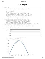
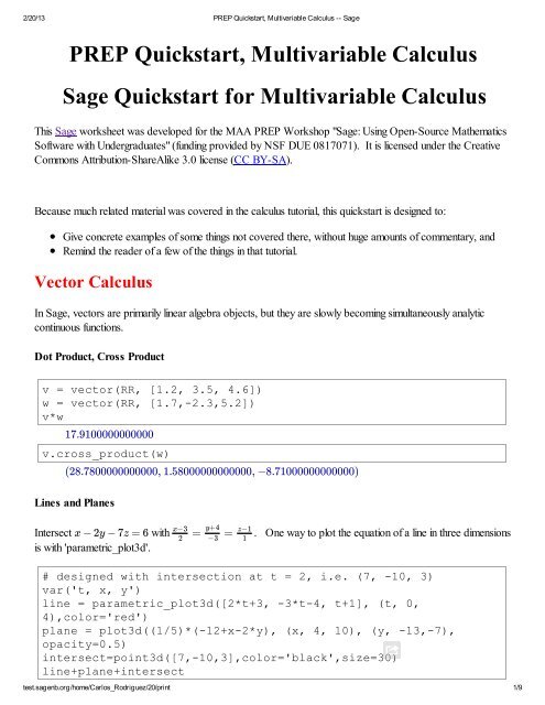
25, )1254(6,2 t, )34 t2 (2,2/20/13 PREP Quickstart, Multivariable Calculus -- SageToggle Advanced ControlsHelp for Jmol 3-D viewerVector-Valued Functionsvar('t')r=vector((2*t-4, t^2, (1/4)*t^3))rr(t=5)(2 t − 4, , ) t 2 1 4 t 3The following makes the derivative also a vector-valued callable expression.velocity = r.diff(t) # velocity(t) = list(r.diff(t)) also wouldworkvelocityvelocity(t=1)test.sagenb.org/home/Carlos_Rodriguez/20/print 2/9(2, 2, )

(2, 2, )3 42/20/13 PREP Quickstart, Multivariable Calculus -- SageIf we know a little vector calculus, we can also do line integrals. Here we compute the arclength betweenand t = π.T=velocity/velocity.norm()t = 0T(t=1).n()(0.683486126173409, 0.683486126173409, 0.256307297315028)We can even then get the arc length by integrating the normalized derivative. As pointed out in the calculustutorial, the syntax for numerical_integral is slightly nonstandard - we just put in the endpoints, not the variable.arc_length = numerical_integral(rprime.norm(), 0,1)arc_lengthTraceback (click to the left of this block for traceback)...NameError: name 'rprime' is not definedIf we know a little vector calculus, we can also do line integrals. Here we compute a number of quantities.var('x,y,t')density(x,y)=x^2+ytstart=0tend=pit_range=(t,tstart,tend)r_prime = diff(r,t)ds=diff(r,t).norm()arclength=integral(ds,t, tstart, tend)To do line integrals, let's make a function that will calculatevarious differentials to to easily specify the dtintegrands.. We'll use our formulas relating# Let's make a function right off to evaluate an integral overthis curve.# this function uses our values of r, tstart, and tenddef line_integral(integrand):return RR(numerical_integral((integrand).subs(x=r[0],y=r[1],z=r[2]), tstart, tend)[0])var('x,y,z,t')r_prime = diff(r,t)∫ (integrand)dttest.sagenb.org/home/Carlos_Rodriguez/20/print 3/9

2/20/13 PREP Quickstart, Multivariable Calculus -- Sageds=diff(r,t).norm()s=line_integral(ds)centroid_x=line_integral(x*ds)/scentroid_y=line_integral(y*ds)/scentroid_z=line_integral(z*ds)/sdm=density(x,y,z)*dsm=line_integral(dm)avg_density = m/smoment_about_yz_plane=line_integral(x*dm)moment_about_xz_plane=line_integral(y*dm)moment_about_xy_plane=line_integral(z*dm)center_mass_x = moment_about_yz_plane/mcenter_mass_y = moment_about_xz_plane/mcenter_mass_z = moment_about_xy_plane/mIx=line_integral((y^2+z^2)*dm)Iy=line_integral((x^2+z^2)*dm)Iz=line_integral((x^2+y^2)*dm)Rx = sqrt(Ix/m)Ry = sqrt(Iy/m)Rz = sqrt(Iz/m)Let's display everything in a nice table.html.table([[r"Density $\delta(x,y)$", density],[r"Curve $\vec r(t)$",r],[r"$t$ range", t_range],[r"$\vec r'(t)$", r_prime],[r"$ds$, a little bit of arclength", ds],[r"$s$ - arclength", s],[r"Centroid (constant density) $\left(\frac{1}{m}\intx\,ds,\frac{1}{m}\int y\,ds, \frac{1}{m}\int z\,ds\right)$",(centroid_x,centroid_y,centroid_z)],[r"$dm=\delta ds$ - a little bit of mass", dm],[r"$m=\int \delta ds$ - mass", m],[r"average density $\frac{1}{m}\int ds$" , avg_density.n()],[r"$M_{yz}=\int x dm$ - moment about $yz$ plane",moment_about_yz_plane],[r"$M_{xz}=\int y dm$ - moment about $xz$ plane",moment_about_xz_plane],[r"$M_{xy}=\int z dm$ - moment about $xy$ plane",moment_about_xy_plane],[r"Center of mass $\left(\frac1m \int xdm, \frac1m \int ydm,\frac1m \int z dm\right)$", (center_mass_x, center_mass_y,test.sagenb.org/home/Carlos_Rodriguez/20/print 4/9

2/20/13 PREP Quickstart, Multivariable Calculus -- Sagecenter_mass_z)],[r"$I_x = \int (y^2+z^2) dm$", Ix],[r"$I_y=\int (x^2+z^2) dm$",Iy],[mp(r"$I_z=\int (x^2+y^2)dm$"), Iz],[r"$R_x=\sqrt{I_x/m}$", Rx],[mp(r"$R_y=\sqrt{I_y/m}"), Ry],[mp(r"$R_z=\sqrt{I_z/m}"),Rz]])Traceback (click to the left of this block for traceback)...NameError: name 'mp' is not definedWe can also plot vector fields, even in three dimensions.x,y,z=var('x y z')plot_vector_field3d((x*cos(z),-y*cos(z),sin(z)), (x,0,pi),(y,0,pi), (z,0,pi),colors=['red','green','blue'])Toggle Advanced ControlsHelp for Jmol 3-D viewerFunctions of Several VariablesThis connects directly to other issues of multivariable functions.How to view these was mostly addressed in the various plotting tutorials. Here is a reminder of what can betest.sagenb.org/home/Carlos_Rodriguez/20/print 5/9

2/20/13 PREP Quickstart, Multivariable Calculus -- Sagedone.# import matplotlib.cm; matplotlib.cm.datad.keys()# 'Spectral', 'summer', 'blues'g(x,y)=e^-x*sin(y)contour_plot(g, (x, -2, 2), (y, -4*pi, 4*pi), cmap = 'Blues',contours=10, colorbar=True)Partial DifferentiationThe following exercise is from Hass, Weir, and Thomas, University Calculus, Exercise 12.7.35. It has a localminimum at .(4,−2)f(x, y) = x^2 + x*y + y^2 - 6*x + 2test.sagenb.org/home/Carlos_Rodriguez/20/print 6/9

↦ 2 x + y − 6(x,y)↦ x + 2 y(x,y)f xxD = 3f xxf xx2/20/13 PREP Quickstart, Multivariable Calculus -- SageQuiz: Why did we not need to declare the variables in this case?fx(x,y)= f.diff(x)fy(x,y) = f.diff(y)fx; fyf.gradient()solve([fx==0, fy==0], (x, y))(x,y) ↦ (2 x + y − 6, x + 2 y)H = f.hessian()H(x,y)[[x = 4,y = (−2)]]2112And of course if the Hessian has positive determinant andis positive, we have a local minimum.( )Notice how we were able to use many things we've done up to now to solve this.MatricesSymbolic functionsSolvingDifferential calculusSpecial formatting commandsAnd, below, plotting!html("$f_{xx}=%s$"%H(4,-2)[0,0])html("$D=%s$"%H(4,-2).det())= 2And of course if the Hessian is positive definite andis positive, we have a local minimum.Notice how we were able to use many things we've done up to now to solve this.test.sagenb.org/home/Carlos_Rodriguez/20/print 7/9

2/20/13 PREP Quickstart, Multivariable Calculus -- SageMatricesSymbolic functionsSolvingDifferential calculusSpecial formatting commandsAnd, below, plotting!plot3d(f,(x,-5,5),(y,-5,5))+point((4,-2,f(4,-2)),color='red',size=20)Toggle Advanced ControlsHelp for Jmol 3-D viewerf(x,y)=x^2*yQuiz: why did we need to declare variables this time?# integrate in the order dy dxf(x,y).integrate(y,0,4*x).integrate(x,0,3)19445# another way to integrate, and in the opposite order toointegrate( integrate(f(x,y), (x, y/4, 3)), (y, 0, 12) )19445var('u v')surface = plot3d(f(x,y), (x, 0, 3.2), (y, 0, 12.3), color =test.sagenb.org/home/Carlos_Rodriguez/20/print 8/9

2/20/13 PREP Quickstart, Multivariable Calculus -- Sage'blue', opacity=0.3)domain = parametric_plot3d([3*u, 4*(3*u)*v,0], (u, 0, 1), (v,0,1), color = 'green', opacity = 0.75)image = parametric_plot3d([3*u, 4*(3*u)*v, f(3*u, 12*u*v)], (u,0, 1), (v, 0,1), color = 'green', opacity = 1.00)surface+domain+imageToggle Advanced ControlsHelp for Jmol 3-D viewertest.sagenb.org/home/Carlos_Rodriguez/20/print 9/9