Introduction to differential forms

Introduction to differential forms
Donu Arapura
This is a supplement for my Math 362 class. The calculus of differential
forms gives an alternative to vector calculus which, although quite compelling,
is rarely taught at this level.
1 1-forms
A differential 1-form (or simply a differential or a 1-form) on an open subset of
R 2 is an expression F (x, y)dx + G(x, y)dy where F, G are R-valued functions on
the open set. A very important example of a differential is given as follows: If
f(x, y) is C 1 R-valued function on an open set U, then its total differential (or
exterior derivative) is
df = ∂f ∂f
dx +
∂x ∂g dy
It is a differential on U.
In a similar fashion, a differential 1-form on an open subset of R 3 is an
expression F (x, y, z)dx + G(x, y, z)dy + H(x, y, z)dz where F, G, H are R-valued
functions on the open set. If f(x, y, z) is a C 1 function on this set, then its total
differential is
df = ∂f
∂x
∂f ∂f
dx + dy +
∂y ∂z dz
At this stage, it is worth pointing out that a differential form is very similar
to a vector field. In fact, we can set up a correspondence:
F i + Gj + Hk ↔ F dx + Gdy + Hdz
Under this set up, the gradient ∇f corresponds to df. Thus it might seem that
all we are doing is writing the previous concepts in a funny notation. However,
the notation is very suggestive and ultimately quite powerful. Suppose that that
x, y, z depend on some parameter t, and f depends on x, y, z, then the chain
rule says
df
dt = ∂f dx
∂x dt + ∂f dy
∂y dt + ∂f dz
∂z dt
Thus the formula for df can be obtained by canceling dt.
1

2 Exactness in R 2
Suppose that F dx + Gdy is a differential on R 2 with C 1 coefficients. We will
say that it is exact if one can find a C 2 function f(x, y) with df = F dx + Gdy
Most differential forms are not exact. To see why, note that the above equation
is equivalent to
F = ∂f
∂x , G = ∂f
∂y .
Therefore if f exists then
∂F
∂y = ∂2 f
∂y∂x = ∂2 f
∂x∂y = ∂G
∂x
But this equation would fail for most examples such as ydx. We will call a
differential closed if ∂F ∂G
∂y
and
∂x
are equal. So we have just shown that if a
differential is to be exact, then it had better be closed.
Exactness is a very important concept. You’ve probably already encountered
it in the context of differential equations. Given an equation
we can rewrite it as
dy
= F (x, y)
dx
F dx − dy = 0
If the differential on the left is exact and equal to say, df, then the curves
f(x, y) = c give solutions to this equation.
These concepts arise in physics. For example given a vector field F =
F 1 i + F 2 j representing a force, one would like find a function P (x, y) called
the potential energy, such that F = −∇P . The force is called conservative (see
section 8) if it has a potential energy function. In terms of differential forms, F
is conservative precisely when F 1 dx + F 2 dy is exact.
3 Parametric curves
Before discussing line integrals, we have to say a few words about parametric
curves. A parametric curve in the plane is vector valued function C : [a, b] → R 2 .
In other words, we let x and y depend on some parameter t running from a to
b. It is not just a set of points, but the trajectory of particle travelling along the
curve. To begin with, we will assume that C is C 1 . Then we can define the the
velocity or tangent vector v = ( dx ). We want to assume that the particle
travels without stopping, v ≠ 0. Then v gives a direction to C, which we also
refer to as its orientation. If C is given by
dt , dy
dt
x = f(t), y = g(t), a ≤ t ≤ b
then
x = f(−u), y = g(−u), −b ≤ u ≤ −a
2

will be called −C. This represents the same set of points, but traveled in the
opposite direction.
Suppose that C is given depending on some parameter t,
x = f(t), y = g(t)
and that t depends in turn on a new parameter t = h(u) such that dt
du ≠ 0.
Then we can get a new parametric curve C ′
x = f(h(u)), y = g(h(u))
It the derivative dt
du
is everywhere positive, we want to view the oriented curves
C and C ′ as the equivalent. If this derivative is everywhere negative, then −C
and C ′ are equivalent. For example, the curves
C : x = cos θ, y = sin θ, 0 ≤ θ ≤ 2π
C ′ : x = sin t, y = cos t, 0 ≤ t ≤ 2π
represent going once around the unit circle counterclockwise and clockwise respectively.
So C ′ should be equivalent to −C. We can see this rigorously by
making a change of variable θ = π/2 − t.
It will be convient to allow piecewise C 1 curves. We can treat these as unions
of C 1 curves, where one starts where the previous one ends. We can talk about
parametrized curves in R 3 in pretty much the same way.
4 Line integrals
Now comes the real question. Given a differential F dx + Gdy, when is it exact
Or equivalently, how can we tell whether a force is conservative or not Checking
that it’s closed is easy, and as we’ve seen, if a differential is not closed, then
it can’t be exact. The amazing thing is that the converse statement is often
(although not always) true:
THEOREM 4.1 If F (x, y)dx + G(x, y)dy is a closed form on all of R 2 with
C 1 coefficients, then it is exact.
To prove this, we would need solve the equation df = F dx + Gdy. In other
words, we need to undo the effect of d and this should clearly involve some kind
of integration process. To define this, we first have to choose a parametric C 1
curve C. Then we define:
DEFINITION 4.2
∫
F dx + Gdy =
C
∫ b
a
[F (x(t), y(t)) dx
dt
+ G(x(t), y(t))
dy
dt ]dt
3

If C is piecewise C 1 , then we simply add up the integrals over the C 1 pieces.
Although we’ve done everything at once, it is often easier, in practice, to do
this in steps. First change the variables from x and y to expresions in t, then
replace dx by dx
dt
dt etc. Then integrate with respect to t. For example, if we
parameterize the unit circle c by x = cos θ, y = sin θ, 0 ≤ θ ≤ 2π, we see
−
y
x 2 + y 2 dx + x
x 2 + y 2 dy = − sin θ(cos θ)′ dθ + cos θ(sin θ) ′ dθ = dθ
and therefore
From the chain rule, we get
LEMMA 4.3
∫
C
−
y
∫
x 2 + y 2 dx + x
2π
x 2 + y 2 dy = dθ = 1
∫
−C
∫
F dx + Gdy = − F dx + Gdy
C
If C and C ′ are equivalent, then
∫
∫
F dx + Gdy =
C
C ′
0
F dx + Gdy
While we’re at it, we can also define a line integral in R 3 . Suppose that
F dx + Gdy + Hdz is a differential form with C 1 coeffients. Let C : [a, b] → R 3
be a piecewise C 1 parametric curve, then
DEFINITION 4.4
∫ b
a
[F (x(t), y(t), z(t)) dx
dt
∫
C
F dx + Gdy + Hdz =
dy
dz
+ G(x(t), y(t), z(t)) + H(x(t), y(t), z(t))
dt dt ]dt
The notion of exactness extends to R 3 automatically: a form is exact if it
equals df for a C 2 function. One of the most important properties of exactness
is its path independence:
C 1
PROPOSITION 4.5 If ω is exact and C 1 and C 2 are two parametrized curves
with the same endpoints (or more acurately the same starting point and ending
point), then
∫ ∫
ω = ω
It’s quite easy to see why this works. If ω = df and C 1 : [a, b] → R 3 then
∫ ∫ b
df
df =
C 1
dt dt
by the chain rule. Now the fundamental theorem of calculus shows that the
last integral equals f(C 1 (b)) − f(C 1 (a)), which is to say the value of f at the
a
C 2
4

endpoint minus its value at the starting point. A similar calculation shows that
the integral over C 2 gives same answer. If the C is closed, which means that
the starting point is the endpoint, then this argument gives
COROLLARY 4.6 If ω is exact and Cis closed, then ∫ C ω = 0.
Now we can prove theorem 4.1. If F dx + Gdy is a closed form on R 2 , set
∫
f(x, y) = F dx + Gdy
where the curve is indicated below:
C
(x,y)
(0,0)
(x,0)
We parameterize both line segments seperately by x = t, y = 0 and x =
x(constant), y = t, and sum to get
f(x, y) =
∫ x
F (t, 0)dt +
∫ y
0
0
G(x, t)dt
Then we claim that df = F dx + Gdy. To see this, we differentiate using the
fundamental theorem of calculus. The easy calcutation is
∂f
∂y
∫ y
= ∂ G(x, t)dt
∂y 0
= G(x, y)
Slightly trickier is
∂f
∂x
∫ x
∫ y
= ∂ F (x, 0)dt + ∂ G(x, t)dt
∂x 0
∂x 0
∫ y
∂G(x, t)
= F (x, 0) +
dt
0 ∂x
∫ y
∂F (x, t)
= F (x, 0) +
dt
0 ∂t
= F (x, 0) + F (x, y) − F (x, 0)
= F (x, y)
5

The same proof works if if we replace R 2 by an open rectangle. However, it
will fail for more general open sets. For example,
−
y
x 2 + y 2 dx + x
x 2 + y 2 dy
is C 1 1-form on the open set {(x, y) | (x, y) ≠ (0, 0)} which is closed. But it is
not exact, since its integral along the unit circle is 0.
5 Work
Line integrals have many important uses. One very direct application in physics
comes from the idea of work. If you pick up a rock off the ground, or perhaps
roll it up a ramp, it takes energy. The energy expended is called work. If you’re
moving the rock in straight line for a short distance, then the displacement can
be represented by a vector d = (∆x, ∆y, ∆z) and the force of gravity by a vector
F = (F 1 , F 2 , F 3). Then the work done is simply
−F · d = −(F 1 ∆x + F 2 ∆y + F 3 ∆z).
On the other hand, if you decide to shoot a rocket up into space, then you would
have to take into account that the trajectory c may not be straight nor can the
force F be assumed to be constant (it’s a vector field). However as the notation
suggests, for the work we would now need to calculate the integral
∫
− F 1 dx + F 2 dy + F 3 dz
One often writes this as
c
∫
− F · ds
c
(think of ds as the “vector” (dx, dy, dz).)
6 2-forms
Recall that the cross product is an operation on vector fields satisfying:
u × v = −v × u (anticommutative law)
u × (v + w) = u × v + u × w (distributive law)
Geometrically u × v represents the vector, perpendicular to the uv-plane,
whose length is the area of the parallelogram spanned by u and v with direction
determined by the right hand rule.
We’ll introduce an operation on 1-forms called the wedge product (written
as ∧) which is analogous to the cross product. One important difference is that
while the cross product of two vectors is again a vector, the wedge product
results a new kind of expression called a 2-form. The wedge product will be
both anticommutative and distributive like the cross product:
6

A typical 2-form looks like this:
α ∧ β = −β ∧ α
α ∧ (β + γ) = α ∧ β + α ∧ γ
F (x, y, z)dx ∧ dy + G(x, y, z)dy ∧ dz + H(x, y, z)dz ∧ dx
where F, G and H are functions defined on an open subset of R 3 . The real
significance of 2-forms will come later when we do surface integrals. A 2-form
will be an expression that can be integrated over a surface in the same way that
a 1-form can be integrated over a curve.
7 “d” of a 1-form and the curl
Given a 1-form F (x, y, z)dx + G(x, y, z)dy + H(x, y, z)dz. We want to define its
derivative dω which will be a 2-form. The rules we use to evaluate it are:
d(α + β) = dα + dβ
d(fα) = (df) ∧ α + fdα
d(dx) = d(dy) = d(dz) = 0
where α and β are 1-forms and f is a function. Putting these together yields a
formula
d(F dx + Gdy + Hdz) = (G x − F y )dx ∧ dy + (H y − G z )dy ∧ dz + (F z − H x )dz ∧ dx
where F x = ∂F
∂x
and so on.
A 2-form can be converted to a vector field by replacing dx ∧ dy by k = i × j,
dy ∧ dz by i = j × k and dz ∧ dx by j = k × i. If we start with a vector field
V = F i + Gj + Hk, replace it by a 1-form F dx + Gdy + Hdz, apply d, then
convert it back to a vector field, we end up with the curl of V
∇ × V = (H y − G z )i + (G x − F y )k + (F z − H x )j
(In practice, one often writes this as a determinant
i j k
∇ × V =
∂ ∂
∂dx ∂dy
∣ F G H
∂
∂dz
∣ .
)
7

8 Exactness in R 3 and conservation of energy
A C 1 1-form ω = F dx + Gdy + Hdz is called exact if there is a C 2 function
(called a potential) such that ω = df. ω is called closed if dω = 0, or equivalently
if
F y = G x , F z = H x , G z = H y
Then exact 1-forms are closed.
THEOREM 8.1 If ω = F dx + Gdy + Hdz is a closed form on R 3 with C 1
coefficients, then ω is exact. In fact if f(x 0 , y o , z 0 ) = ∫ ω, where C is any
C
piecewise C 1 curve connecting (0, 0, 0) to (x 0 , y 0 , z 0 ), then df = ω.
This can be rephrased in the language of vector fields. If F = F i + Gj + Hk
is C 1 vector field representing a force, then it is called conservative if there is a
C 2 real valued function P , called potential energy, such that F = −∇P . The
theorem implies that a force F, which is C 1 on all of R 3 , is conservative if and
only if ∇ × F = 0. P (x, y, z) is just the work done by moving a particle of unit
mass along a path connecting (0, 0, 0) to (x, y, z).
To appreciate the importance of this concept, recall from physics that the
kinetic energy of a particle of constant mass m and velocity
is
v = ( dx
dt , dy
dt , dz
dt )
K = 1 2 m||v||2 = 1 mv · v.
2
Also one of Newton’s laws says
m dv
dt = F
If F is conservative, then we can replace it by −∇P above, move it to the other
side, and then dot both sides by v to obtain
mv · dv
dt + v · ∇P = 0
which simplifies 1 to
d
(K + P ) = 0.
dt
This implies that the total energy K + P is constant.
1 This takes a bit of work that I’m leaving as an exercise. It’s probably easier to work
backwards. You’ll need the product rule for dot products and the chain rule.
8

9 “d” of a 2-form and divergence
A 3-form is simply an expression f(x, y, z)dx ∧ dy ∧ dz. These are things that
will eventually get integrated over solid regions. The important thing for the
present is an operation which takes 2-forms to 3-forms once again denoted by
“d”.
d(F dy ∧ dz + Gdz ∧ dx + Hdx ∧ dy) = (F x + G y + H z )dx ∧ dy ∧ dz
It’s probably easier to understand the pattern after converting the above 2-
form to the vector field V = F i + Gj + Hk. Then the coeffiecient of dx ∧ dy ∧ dz
is the divergence
∇ · V = F x + G y + H z
So far we’ve applied d to functions to obtain 1-forms, and then to 1-forms to
get 2-forms, and finally to 2-forms. The real power of this notation is contained
in the following simple-looking formula
PROPOSITION 9.1 d 2 = 0
What this means is that given a C 2 real valued function defined on an open
subset of R 3 , then d(df) = 0, and given a 1-form ω = F dx + Gdy + Hdz with
C 2 coefficents defined on an open subset of R 3 , d(dω) = 0. Both of these are
quite easy to check:
d(df) = (f yx − f xy )dx ∧ dy + (f zy − f yz )dy ∧ dz + (f xz − f zx )dz ∧ dx = 0
d(dω) = [G xz − F yz + H yx − G zx + F zy − H xy ]dx ∧ dy ∧ dz = 0
In terms of standard vector notation this is equivalent to
The analogue of theorem 8.1 holds:
∇ × (∇f) = 0
∇ · (∇ × V) = 0
THEOREM 9.2 If ω is a 2-form on R 3 such that dω = 0, then there exists a
1-form ξ such that dξ = ω.
10 Parameterized Surfaces
Recall that a parameterized curve is a C 1 function from a interval [a, b] ⊂ R 1 to
R 3 . If we replace the interval by subset of the plane R 2 , we get a parameterized
surface. Let’s look at a few of examples
1) The upper half sphere of radius 1 centered at the origin can be parameterized
using cartesian coordinates
⎧
⎪⎨
⎪⎩
x = u
y = v
z = √ 1 − u 2 − v 2
u 2 + v 2 ≤ 1
9

2) The upper half sphere can be parameterized using spherical coordinates
⎧
x = sin(φ) cos(θ)
⎪⎨
y = sin(φ) sin(θ)
z = cos(φ)
⎪⎩
0 ≤ φ ≤ π/2, 0 ≤ θ < 2π
3) The upper half sphere can be parameterized using cylindrical coordinates
⎧
x = r cos(θ)
⎪⎨
y = r sin(θ)
z = √ 1 − r ⎪⎩
2
0 ≤ r ≤ 1, 0 ≤ θ < 2π
An orientation on a curve is a choice of a direction for the curve. For a
surface an orientation is a choice of “up” or “down”. The easist way to make
this precise is to view an orientation as a choice of (an upward or outward
pointing) unit normal vector field n on S. A parameterized surface S
⎧
x = f(u, v)
⎪⎨
y = g(u, v)
z = h(u, v)
⎪⎩
(u, v) ∈ D
is called smooth provided that f, g, h are C 1 , the function that they define from
D → R 3 is one to one, and the tangent vector fields
T u = ( ∂x
∂u , ∂y
∂u , ∂z
∂u )
T v = ( ∂x
∂v , ∂y
∂v , ∂z
∂v )
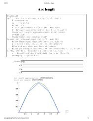
are linearly independent. In this case, once we pick an ordering of the variables
(say u first, v second) an orientation is determined by the normal
n =
T u × T v
||T u × T v ||
10

n
T v
T
u
S
v=constant
u=constant
FIGURE 1
If we look at the examples given earlier. (1) is smooth. However there is
a slight problem with our examples (2) and (3). Here T θ = 0, when φ = 0 in
example (2) and when r = 0 in example (3). To deal with scenario, we will
consider a surface smooth if there is at least one smooth parameterization for
it.
Let C be a closed C 1 curve in R 2 and D be the interior of C. D is an example
of a surface with a boundary C. In this case the surface lies flat in the plane,
but more general examples can be constructed by letting S be a parameterized
surface ⎧⎪ x = f(u, v)
⎨
y = g(u, v)
⎪ z = h(u, v)
⎩
(u, v) ∈ D ⊂ R 2
then the image of C in R 3 will be the boundary of S. For example, the boundary
of the upper half sphere S
⎧
⎪⎨
⎪⎩
x = sin(φ) cos(θ)
y = sin(φ) sin(θ)
z = cos(φ)
0 ≤ φ ≤ π/2, 0 ≤ θ < 2π
11

is the circle C given by
x = cos(θ), y = sin(θ), z = 0, 0 ≤ θ ≤ 2π
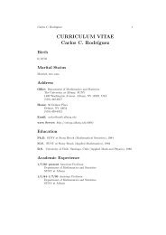
In what follows, we will need to match up the orientation of S and its boundary
curve. This will be done by the right hand rule: if the fingers of the right hand
point in the direction of C, then the direction of the thumb should be “up”.
n
S
C
FIGURE 2
11 Surface Integrals
Let S be a smooth parameterized surface
⎧
x = f(u, v)
⎪⎨
y = g(u, v)
z = h(u, v)
⎪⎩
(u, v) ∈ D
with orientation corresponding to the ordering u, v. The symbols dx etc. can
be converted to the new coordinates as follows
dx = ∂x ∂x
du +
∂u ∂v dv
dx ∧ dy = ( ∂x
∂u
dy = ∂y ∂y
du +
∂u ∂v dv
du +
∂x
∂v
12
∂y ∂y
dv) ∧ ( du +
∂u ∂v dv)

= ( ∂x ∂y
∂u ∂v − ∂x ∂y
)du ∧ dv
∂v ∂u
∂(x, y)
= du ∧ dv
∂(u, v)
In this way, it is possible to convert any 2-form ω to uv-coordinates.
DEFINITION 11.1 The integral of a 2-form on S is given by
∫ ∫
∫ ∫
∂(x, y) ∂(y, z) ∂(z, x)
F dx∧dy+Gdy∧dz+Hdz∧dx = [F +G +H
∂(u, v) ∂(u, v) ∂(u, v) ]dudv
S
In practice, the integral of a 2-form can be calculated by first converting it
to the form f(u, v)du ∧ dv, and then evaluating ∫ ∫ D
f(u, v) dudv.
Let S be the upper half sphere of radius 1 oriented with the upward normal
parameterized using spherical coordinates, we get
So
dx ∧ dy =
∫ ∫
S
dx ∧ dy =
D
∂(x, y)
dφ ∧ dθ = cos(φ) sin(φ)dφ ∧ dθ
∂(φ, θ)
∫ 2π ∫ π/2
0
0
cos(φ) sin(φ)dφdθ = π
On the other hand if use the same surface parameterized using cylindrical
coordinates
∂(x, y)
dx ∧ dy = dr ∧ dθrdr ∧ dθ
∂(r, θ)
Then
∫ ∫
S
dx ∧ dy =
∫ 2π ∫ 1
0
0
rdrdθ = π
which leads to the same answer as one would hope. The general result is:
THEOREM 11.2 Suppose that a oriented surface S has two different smooth
C 1 parameterizations, then for any 2-form ω, the expression for the integrals of
ω calculated with respect to both parameterizations agree.
(This theorem needs to be applied to the half sphere with the point (0, 0, 1)
removed in the above examples.)
12 Triangulation
Complicated surfaces may be divided up into nonoverlapping patches which can
be parameterized separately. The simplest scheme for doing this is to triangulate
the surface, which means that we divide it up into triangular patches as depicted
below. Each triangle on the surface can be parameterized by a triangle on the
plane.
13

oundary
We will insist that if any two triangles touch, they either meet only at a
vertex, or they share an entire edge. We define the boundary of a surface to be
the union of all edges which are not shared. The surface is called closed if the
boundary is empty.
Given a surface which has been divided up into patches, we can integrate a
2-form on it by summing up the integrals over each patch. However, we require
that the orientations match up, which is possible if the surface has “two sides”.
Below is a picture of a one sided, or nonorientable, surface called the Mobius
strip.
Once we have pick and orientation of S, we get one for the boundary using
the right hand rule.
14

13 Flux
In many situations arising in physics, one needs to integrate a vector field F =
F 1 i + F 2 j + F 3 k over a surface. The resulting quantity is often called a flux.
We will simply define this integral, which is usually written as ∫ ∫ ∫ ∫
F · dS or
S
S
F · n dS, to mean
∫ ∫
F 1 dy ∧ dz + F 2 dz ∧ dx + F 3 dx ∧ dy
S
It is probally easier to view this as a two step process, first convert F to a 2-form
as follows:
F 1 i + F 2 j + F 3 k ↔ F 1 dy ∧ dz + F 2 dz ∧ dx + F 3 dx ∧ dy,
then integrate. Earler, we learned how to convert a vector field to a 1-form:
F 1 i + F 2 j + F 3 k ↔ F 1 dx + F 2 dy + F 3 dz
To complete the triangle, we can convert a 1-form to a 2-form and back via:
F 1 dx + F 2 dy + F 3 dz ↔ F 1 dy ∧ dz + F 2 dz ∧ dx + F 3 dx ∧ dy
This operation is usually denoted by ∗.
As a typical example, consider a fluid such as air or water. Associated to
this, there is a scalar field ρ(x, y, z) which measures the density, and a vector
field v which measures the velocity of the flow (e.g. the wind velocity). Then
the ∫ ∫ rate at which the fluid passes through a surface S is given by the flux integral
ρv · dS
S
14 Green’s and Stokes’ Theorems
Stoke’s theorem is really the fundamental theorem of calculus of surface integrals.
We assume that surfaces can triangulated.
THEOREM 14.1 (Stokes’ theorem) Let S be an oriented smooth surface
with smooth boundary curve C. If C is oriented using the right hand rule, then
for any C 1 1-form ω on an open set of R 3 containing S,
∫ ∫ ∫
dω = ω
S
If the surface lies in the plane, it is possible make this very explicit:
THEOREM 14.2 (Green’s theorem) Let C be a closed C 1 curve in R 2 oriented
counterclockwise and D be the interior of C. If P (x, y) and Q(x, y) are
both C 1 functions then
∫
C
∫ ∫
P dx + Qdy =
D
C
( ∂Q
∂y − ∂P
∂x )dxdy
15

As an application, Green’s theorem shows that the area of D can be computed
as line integral on the boundary
∫ ∫ ∫
dxdy = ydx
D
If S is a closed oriented surface in R 3 , such as the surface of a sphere, Stoke’s
theorem show that any exact 2-form integrates to 0. To see this write S as the
union of two surfaces S 1 and S 2 with common boundary curve C. Orient C
using the right hand rule with respect to S 1 , then orientation comming from S 2
goes in the opposite direction. Therefore
∫ ∫ ∫ ∫ ∫ ∫ ∫ ∫ ∫ ∫
dω = dω + dω = ω − ω = 0
S
S 1 S 2 C
C
In vector notation, Stokes’ theorem is written as
∫ ∫
∫
∇ × F · n dS = F · ds
S
where F is a C 1 -vector field.
In physics, there a two fundamental vector fields, the electric field E and the
magnetic field B. They’re governed by Maxwell’s equations, one of which is
C
∇ × E = − ∂B
∂t
where t is time. If we integrate both sides over S, apply Stokes’ theorem and
simplify, we obtain Faraday’s law of induction:
∫
E · ds = − ∂ ∫ ∫
B · n dS
C ∂t
To get a sense of what this says, imagine that C is wire loop and that we are
dragging a magnet through it. This action will induce an electric current; the
left hand integral is precisely the induced voltage and the right side is related to
the strength of the magnet and the rate at which it is being dragged through.
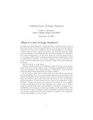
Stoke’s theorem works even if the boundary has several components. However,
the inner an outer components would have opposite directions.
S
C
C
2
S
C
1
16

THEOREM 14.3 (Stokes’ theorem II) Let S be an oriented smooth surface
with smooth boundary curves C 1 , C 2 . . .. If C i is oriented using the right
hand rule, then for any C 1 1-form ω on an open set of R 3 containing S,
∫ ∫ ∫ ∫
dω = ω + ω + . . .
C 1 C 2
S
15 Triple integrals and the divergence theorem
A 3-form is an expression f(x, y, z)dx ∧ dy ∧ dz. Given a solid region V ⊂ R 3 ,
we define
∫ ∫ ∫
∫ ∫ ∫
f(x, y, z)dx ∧ dy ∧ dz = f(x, y, z)dxdydz
V
THEOREM 15.1 (Divergence theorem) Let V be the interior of a smooth
closed surface S oriented with the outward pointing normal. If ω is a C 1 2-form
on an open subset of R 3 containing V , then
∫ ∫ ∫ ∫ ∫
dω = ω
In standard vector notation, this reads
∫ ∫ ∫
∫ ∫
∇ · F dV =
V
V
S
S
V
F · n dS
where F is a C 1 vector field.
As an application, consider a fluid with density ρ and velocity v. If S is the
∫boundary ∫ of a solid region V with outward pointing normal n, then the flux
S
ρv · n dS is the rate at which matter flows out of V . In other words, it is
minus the rate at which matter flows in, and this equals −∂/∂t ∫ ∫ ∫ ρdV . On
V
∫the ∫ ∫other hand, by the divergence theorem, the above double integral equals
∇ · (ρv) dV . Setting these equal and subtracting yields
S
∫ ∫ ∫
V
[∇ · (ρv) + ∂ρ ] dV = 0.
∂t
The only way this can hold for all possible regions V is that the integrand
∇ · (ρv) + ∂ρ
∂t = 0
This is one of the basic laws of fluid mechanics.
We can extend the divergence theorem to solids with disconnected boundary.
Suppose that S 2 is a smooth closed oriented surface contained inside another
such surface S 1 . We use the outward pointing normal S 1 and the inner pointing
normal on S 2 . Let V be region in between S 1 and S 2 . Then,
THEOREM 15.2 (Divergence theorem II) If ω is a C 1 2-form on an open
subset of R 3 containing V , then
∫ ∫ ∫ ∫ ∫ ∫ ∫
dω = ω + ω
S 1 S 2
V
17

16 Gravitational Flux
Place a “point particle” of mass m at the origin of R 3 , then this generates a
force on any particle of unit mass at r = (x, y, z) given by
F = −mr
r 3
where r = ||r|| = √ x 2 + y 2 + z 2 . This has singularity at 0, so it is a vector field
on R 3 − {0}. The corresponding 2-form is given by
ω = −m
xdy ∧ dz + ydz ∧ dx + zdx ∧ dy
r 3
Let B R be the ball of radius R around 0, and let S R be its boundary. Since the
outward unit normal to S R is just n = r/r. One might expect that the flux
∫ ∫S R
F · ndS = − m R 2 ∫ ∫
S R
dS
= − m R 2 area(S R) = − m R 2 (4πR2 )
However, this is really just a proof by notation at this point. To justify it, we
work in spherical coordinates. S R is given by
⎧
⎪⎨
⎪⎩
x = R sin(φ) cos(θ)
y = R sin(φ) sin(θ)
z = R cos(φ)
0 ≤ φ ≤ π, 0 ≤ θ < 2π
Rewriting ω in these coordinates and simplifying:
ω = −mR 3 sin(φ)dφ ∧ dθ
Therefore,
∫ ∫
∫ ∫
F · ndS = ω = −4πm
S R S R
as hoped. We claim that if S is any closed surface not containing 0
∫ ∫ { −4πm if 0 lies in the interior of S
ω =
S
0 otherwise
By direct calculation, we see that dω = 0. Therefore, the divergence theorem
yields
∫ ∫ ∫ ∫ ∫
ω = dω = 0
S
if the interior V does not contain 0. On the other hand, if V contains 0, let B R
be a small ball contained in V , and let V − B R denote part of V lying outside
of B R . We use the second form of the divergence theorem
∫ ∫ ∫ ∫ ∫ ∫ ∫ ∫
ω − ω = ω = 0
S
S R V −B R
18
V

We are subtracting the second surface integral, since we are suppose to use the
inner normal for S R . Thus ∫ ∫
ω = −4πm
S
Incidentally, this shows that ω is not exact. Thus theorem 9.2 fails for R 3 −{0}.
From here, we can easily extract an expression for the flux for several particles
or even a continuous distribution of matter. If F is the force of gravity
associated to some mass distribution, then for any closed surface S oriented by
the outer normal, then the flux
∫ ∫
F · ndS
S
is −4π times the mass inside S. For a continuous distribution with density ρ,
this is given by ∫ ∫ ∫ ρdV . Applying the divergence theorem again, in this case,
yields
∫ ∫ ∫
(∇ · F + 4πρ)dV = 0
for all regions V . Therefore
17 Beyond R 3
V
∇ · F = −4πρ
It is possible to do calculus in R n with n > 3. Here the language of differential
forms comes into its own. While it would be impossible to talk about the
curl of a vector field in, say, R 4 , the derivative of a 1-form or 2-form presents
no problems; we simply apply the rules we’ve already learned. Integration
over higher dimensional “surfaces” or manifolds can be defined, and there is an
analogue of Stokes’ theorem in this setting.
As exotic as all of this sounds, there are applications of these ideas outside
of mathematics. For example, in relativity theory one needs to treat the electric
E = E 1 i + E 2 j + E 3 k and magnetic fields B = B 1 i + B 2 j + B 3 k as part of a
single “field” on space-time. In mathematical terms, we can take space-time to
be R 4 - with the fourth coordinate as time t. The electromagnetic field can be
represented by a 2-form
F = B 3 dx ∧ dy + B 1 dy ∧ dz + B 2 dz ∧ dx + E 1 dx ∧ dt + E 2 dy ∧ dt + E 3 dz ∧ dt
If we compute dF using the analogues of the rules we’ve learned:
dF = ( ∂B 3
∂x dx + ∂B 3
∂y dy + ∂B 3
∂z dz + ∂B 3
dt) ∧ dx ∧ dy + . . .
∂t
= ( ∂B 1
∂x + ∂B 2
∂y + ∂B 3
∂z )dx ∧ dy ∧ dz + ( ∂E 2
∂x − ∂E 1
∂y + ∂B 3
)dx ∧ dy ∧ dt + . . .
∂t
19

Two of Maxwell’s equations
∇ · B = 0, ∇ × E = − ∂B
∂t
can be expressed very succintly in this language as dF = 0. The analogue of
theorem 9.2 holds for R n , and shows that
F = d(A 1 dx + A 2 dy + A 3 dy + A 4 dt)
for some 1-form called the potential. Thus we’ve reduced the 6 quantites to just
4.
18 Further reading
For more information about differential forms, see the books “Differential forms
and applications to the physical sciences” by H. Flanders and “Calculus on
manifolds” by M. Spivak. All the physics background can be found in “Lectures
on Physics” by R. Feynman et. al.
20