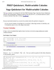
Introduction to differential forms

2 Exactness in R 2
Suppose that F dx + Gdy is a differential on R 2 with C 1 coefficients. We will
say that it is exact if one can find a C 2 function f(x, y) with df = F dx + Gdy
Most differential forms are not exact. To see why, note that the above equation
is equivalent to
F = ∂f
∂x , G = ∂f
∂y .
Therefore if f exists then
∂F
∂y = ∂2 f
∂y∂x = ∂2 f
∂x∂y = ∂G
∂x
But this equation would fail for most examples such as ydx. We will call a
differential closed if ∂F ∂G
∂y
and
∂x
are equal. So we have just shown that if a
differential is to be exact, then it had better be closed.
Exactness is a very important concept. You’ve probably already encountered
it in the context of differential equations. Given an equation
we can rewrite it as
dy
= F (x, y)
dx
F dx − dy = 0
If the differential on the left is exact and equal to say, df, then the curves
f(x, y) = c give solutions to this equation.
These concepts arise in physics. For example given a vector field F =
F 1 i + F 2 j representing a force, one would like find a function P (x, y) called
the potential energy, such that F = −∇P . The force is called conservative (see
section 8) if it has a potential energy function. In terms of differential forms, F
is conservative precisely when F 1 dx + F 2 dy is exact.
3 Parametric curves
Before discussing line integrals, we have to say a few words about parametric
curves. A parametric curve in the plane is vector valued function C : [a, b] → R 2 .
In other words, we let x and y depend on some parameter t running from a to
b. It is not just a set of points, but the trajectory of particle travelling along the
curve. To begin with, we will assume that C is C 1 . Then we can define the the
velocity or tangent vector v = ( dx ). We want to assume that the particle
travels without stopping, v ≠ 0. Then v gives a direction to C, which we also
refer to as its orientation. If C is given by
dt , dy
dt
x = f(t), y = g(t), a ≤ t ≤ b
then
x = f(−u), y = g(−u), −b ≤ u ≤ −a
2