Chapter 10 Continuous probability distributions - Ugrad.math.ubc.ca

More documents

Recommendations

Info

$Math 103, Section 203, Spring Term 2004, Midterm # 1 (35 min ...$

Math 103 Notes Chapter 10Now as T → ∞, we haveI T =[−Te −kT − e−kT+ 1 ].k kTe −kT → 0, e −kT → 0so that¯t = lim I T = 1T →∞ k .Thus the mean or expected decay time is¯t = 1 k .10.5 Discrete versus continuous probabilityIn an earlier chapter, we compared the treatment of two types of mass distributions. We firstexplored a set of discrete masses strung along a “thin wire”. Later, we considered a single “bar”with a continuous distribution of density along its length. In the first case, there was an unambiguousmeaning to the concept of “mass at a point”. In the second case, we could assign a mass to somesection of the bar between, say x = a and x = b. (To do so we had to integrate the mass density onthe interval a ≤ x ≤ b.) In the first case, we talked about the mass of the objects, whereas in thelatter case, we were interested in the idea of density (mass per unit distance: Note that the unitsof mass density are not the same as the units of mass.)The same dichotomy exists in the topic of probability. In an earlier chapter, we were concernedwith the probability of discrete events whose outcome belongs to some finite set of possibilities (e.g.Head or Tail for a coin toss, allele A or a in genetics). But many random processes lead to aninfinite, continuous set of possible outcomes. We need the notion of continuous probability to dealwith such cases. In continuous probability, we consider the probability density - analogous to massdensity. We can assign a probability to some range of values of the outcome between x = a andx = b. (To do so we have to integrate the probability density on the interval a ≤ x ≤ b.)The examples below provide some further insight to the connection between continuous anddiscrete probability. In particular, we will see that one can arrive at the idea of probability densityby refining a set of measurements and making the appropriate scaling. We explore this connectionin more detail below.10.5.1 Example: Student heightsSuppose we measure the heights of all UBC students. This would produce about 30,000 datavalues. We could make a graph and show how these heights are distributed. For example, we couldsubdivide the student body into those students between 0 and 1.5m, and those between 1.5 and 3meters. Our bar graph would contain two bars, with the number of students in each height categoryrepresented by the heights of the bars, as shown in Figure 10.3(a).Suppose we want to keep more detail. We could divide the population into smaller groups byshrinking the size of the interval or “bin” into which height is subdivided. (An example is shownv.2005.1 - January 5, 2009 10
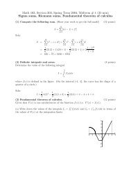
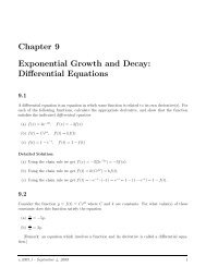
Math 103 Notes Chapter 10p(h)p(h)p(h)∆ hh∆ hhhFigure 10.3: Refining a histogram by increasing the number of bins leads (eventually) to the ideaof a continuous probability density.in Figure 10.3(b)). Here, by a “bin” we mean a little interval of width ∆h where h is height, i.e. aheight interval. For example, we could keep track of the heights in increments of 50 cm. If we wereto plot the number of students in each height category, then as the size of the bins gets smaller,so would the height of the bar: there would be fewer students in each category if we increase thenumber of categories.To keep the bar height from shrinking, we might reorganize the data slightly. Instead of plottingthe number of students in each bin, we might plotnumber of students in bin.∆hIf we do this, then both numerator and denominator decrease as the size of the bins is made smaller,so that the shape of the distribution is preserved (i.e. it does not get flatter).We observe that in this case, the number of students in a given height category is representedby the area of the bar corresponding to that category:( )number of students in binArea of bin = ∆h= number of students in bin.∆hThe important point to consider is that the height of each bar in the plot represents the number ofstudents per unit height.This type of plot is precisely what leads us to the idea of a density distribution. As ∆h shrinks,we get a continuous graph. If we “normalize”, i.e. divide by the total area under the graph, we geta probability density, p(h) for the height of the population. As noted, p(h) represents the fractionof students per unit height whose height is h. It is thus a density, and has the appropriate units.More generally,p(x) ∆xrepresents the fraction of individuals whose height is in the range x ≤ h ≤ x + ∆x.10.5.2 Examples: Age dependent mortalityLet p(a) be a probability density for the probability of mortality of a female Canadian non-smoker atage a, where 0 ≤ a ≤ 120. (We have chosen an upper endpoint of age 120 since practically no Canav.2005.1- January 5, 2009 11
Page 1 and 2: Chapter 10Continuous probability di
Page 3 and 4: Math 103 Notes Chapter 10Finding th
Page 5 and 6: Math 103 Notes Chapter 10Definition
Page 7: Math 103 Notes Chapter 10Figure 10.
Page 12 and 13: Math 103 Notes Chapter 10dian femal
Page 14 and 15: Math 103 Notes Chapter 10(a) The de
Page 16 and 17: Math 103 Notes Chapter 10up to the
Page 18 and 19: Math 103 Notes Chapter 10ThusV = M

Chapter 10 Continuous probability distributions - Ugrad.math.ubc.ca

Create successful ePaper yourself

Delete template?

Save as template?