Chapter 10 Continuous probability distributions - Ugrad.math.ubc.ca

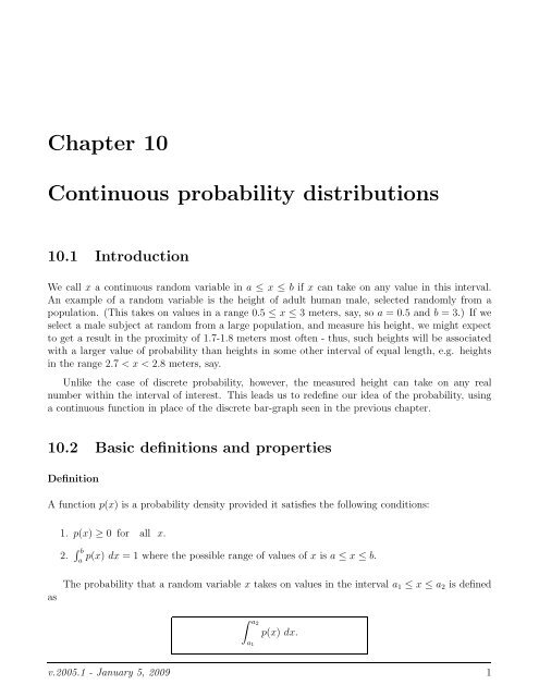
Chapter 10Continuous probability distributions10.1 IntroductionWe call x a continuous random variable in a ≤ x ≤ b if x can take on any value in this interval.An example of a random variable is the height of adult human male, selected randomly from apopulation. (This takes on values in a range 0.5 ≤ x ≤ 3 meters, say, so a = 0.5 and b = 3.) If weselect a male subject at random from a large population, and measure his height, we might expectto get a result in the proximity of 1.7-1.8 meters most often - thus, such heights will be associatedwith a larger value of probability than heights in some other interval of equal length, e.g. heightsin the range 2.7 < x < 2.8 meters, say.Unlike the case of discrete probability, however, the measured height can take on any realnumber within the interval of interest. This leads us to redefine our idea of the probability, usinga continuous function in place of the discrete bar-graph seen in the previous chapter.10.2 Basic definitions and propertiesDefinitionA function p(x) is a probability density provided it satisfies the following conditions:1. p(x) ≥ 0 for all x.2. ∫ bp(x) dx = 1 where the possible range of values of x is a ≤ x ≤ b.aasThe probability that a random variable x takes on values in the interval a 1 ≤ x ≤ a 2 is defined∫ a2a 1p(x) dx.v.2005.1 - January 5, 2009 1

Math 103 Notes Chapter 10Unlike our previous discrete probability, we will not ask “what is the probability that x takeson some exact value?” Rather, we ask for the probability that x is within some range of values,and this is computed by performing an integral. (Remark: the probability that x is exactly equalto b is the integral∫ bbp(x) dx = 0; the value is zero, by properties of the definite integral.)DefinitionThe cumulative distribution function F(x) represents the probability that the random variable takeson any value up to x, i.e.F(x) =∫ xap(s) ds.The cumulative distribution is simply the area under the probability density.The above definition has several implications:Properties of continuous probability1. Since p(x) ≥ 0, the cumulative distribution is an increasing function.2. The connection between the probability density and its cumulative distribution can be written(using the Fundamental Theorem of Calculus) as3. F(a) = 0. This follows from the fact thatp(x) = F ′ (x).F(a) =∫ aBy a property of the definite integral, this is zero.4. F(b) = 1. This follows from the fact thatap(s) ds.by property 2 of p(x).F(b) =∫ bap(s) ds = 15. The probability that x takes on a value in the interval a 1 ≤ x ≤ a 2 is the same asF(a 2 ) − F(a 1 ).This follows from the additive property of integrals:∫ a2p(s) ds −∫ a1p(s) ds =∫ a2aaa 1p(s) dsv.2005.1 - January 5, 2009 2

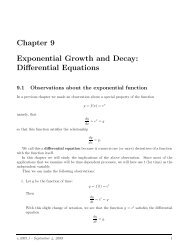
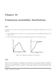
Math 103 Notes Chapter 10Finding the normalization constantNot every function can represent a probability density. For one thing, the function must be positiveeverywhere. Further, the total area under its graph should be 1, by property 2 of a probabilitydensity. However, in many cases we can convert a function to a probability density by simplymultiplying it by a constant, C, equivalent to the reciprocal of the total area under its graph overthe interval of interest. This process is called “normalization”, and the constant C is called thenormalization constant.10.2.1 ExampleConsider the function f(x) = sin(πx/6) for 0 ≤ x ≤ 6.(a) Normalize the function so that it describes a probability density.(b) Find the cumulative distribution function, F(x).SolutionThe function is positive in the interval 0 ≤ x ≤ 6, so we can define the desired probability density.Letp(x) = C sin( π 6 x).(a) We must find the normalization constant, C, such thatHere is how we find the constant:1 =∫ 60∫ 60p(x) dx = 1.C sin( π 6 x) dx = C 6 π(− cos( π 6 x) ) ∣ ∣ ∣∣61 = C 6 12(− cos(π) + cos(0)) = Cπ πThus, we find that the desired constant of normalization isC = π 12 .Once we rescale our function by this constant, we get the desired probability density,p(x) = π 12 sin(π 6 x).This density has the property that the total area under its graph over the interval 0 ≤ x ≤ 6 is 1.A graph of this probability density function is shown in Figure 10.1(a).(b)F(x) =∫ x0p(s) ds = π 12∫ x0sin( π s) ds6v.2005.1 - January 5, 2009 30

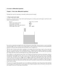
Math 103 Notes Chapter 10F(x) = π (− 6 ) ∣ ∣∣∣x12 π cos(π 6 s) = 1 (1 − cos( π )02 6 x) .This cumulative distribution function is shown in Figure 10.1(b).10.250.20.80.150.60.10.40.050.201 2 3 4 5 601 2 3 4 5 6xxFigure 10.1: (a) The probability density p(x), (left) and (b) the cumulative distribution F(x) (right)for example 1.10.3 Mean and medianRecall that we have defined the mean of a distribution of grades or mass in a previous chapter. Fora mass density ρ(x), the idea of the mean coincides with the center of mass of the distribution,¯x =∫ ba∫ baxρ(x) dx.ρ(x) dxThis definition can also be applied to a probability∫density, but in this case the integral in thebdenominator is simply 1 (by property 2), i.e. p(x) dx = 1. (The simplification is analogous toaan observation we made for expected value in a discrete probability distribution.)We define the mean of a probability density as follows:DefinitionFor a random variable in a ≤ x ≤ b and a probability density p(x) defined on this interval, themean or average value of x (also called the expected value), denoted ¯x is given by¯x =∫ baxp(x) dx.The idea of median encountered previously in grade distributions also has a parallel here. Simplyput, the median is the value of x that splits the probability distribution into two portions whoseareas are identical.v.2005.1 - January 5, 2009 4

Math 103 Notes Chapter 10DefinitionThe median x m of a probability distribution is a value of x in the interval a ≤ x m ≤ b such that∫ xmap(x) dx =∫ bx mp(x) dx = 1 2 .It follows from this definition that the median is the value of x for which the cumulative distributionsatisfiesF(x m ) = 1 2 .10.3.1 ExampleFind the mean and the median of the probability distribution found in Example 10.2.1.SolutionTo find the mean we compute¯x = π 12∫ 60x sin( π x) dx.6Integration by parts is required here. Let u = x, dv = sin( πx) dx. Then du = dx, v = − 6 6 π cos(πx)6The result is(¯x = π −x 6 ∣ ∣∣∣612 π cos(π 6 x) + 6 ∫ )6cos( π0π 0 6 x)dx(¯x = 1 −x cos( π ∣ ∣∣∣62 6 x) + 6 ∣ )∣∣∣6π sin(π 6 x)¯x = 1 (−6 cos(π) + 6 2 π sin(π) − 6 )π sin(0) = 6 2 = 300To find the median, x m , we setF(x m ) = 1 2 .Using the form of the cumulative distribution from example 1, we find that1(1 − cos( π )2 6 x m) = 1 2 .1 − cos( π 6 x m) = 1v.2005.1 - January 5, 2009 5

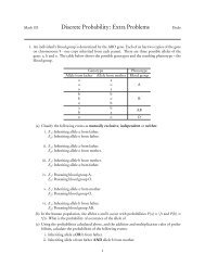
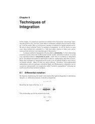
Math 103 Notes Chapter 10cos( π 6 x m) = 0The angles whose cosine is zero are ±π/2, ±3π/2 etc. We select the angle in the relevant interval,i.e. π/2. This leads toπ6 x m = π 2so the median isx m = 3.RemarkA glance at the original probability distribution should convince us that it is symmetric about thevalue x = 3. Thus we should have anticipated that the mean and median of this distribution wouldboth occur at the same place, i.e. at the midpoint of the interval. This will be true in general forsymmetric probability distributions, just as it was for symmetric mass or grade distributions.10.3.2 How is the mean different from the median?p(x)p(x)xxFigure 10.2:We have seen in Example 2 that for symmetric distributions, the mean and the median arethe same. Is this always the case? When are the two different, and how can we understand thedistinction?Recall that the mean is closely associated with the idea of a center of mass, a concept from physicsthat describes the location of a pivot point at which the entire “mass” would exactly balance. It isworth remembering thatmean of p(x) = expected value of x = average value of x.This concept is not to be confused with the average value of a function, which is an average valueof the y coordinate.The median simply indicates a place at which the “total mass” is subdivided into two equalportions. (In the case of probability density, each of those portions represents an equal area,A 1 = A 2 = 1/2 since the total area under the graph is 1 by definition.)v.2005.1 - January 5, 2009 6

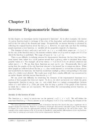
Math 103 Notes Chapter 10Figure 10.2 shows how the two concepts of median (indicated by vertical line) and mean (indicatedby triangular “pivot point”) differ. At the left, for a symmetric probability density, themean and the median coincide, just as they did in Example 2. To the right, a small portion of thedistribution was moved off to the far right. This change did not affect the location of the median,since the areas to the right and to the left of the vertical line are still equal. However, the fact thatpart of the mass is farther away to the right leads to a shift in the mean of the distribution, tocompensate for the change.Simply put, the mean contains more information about the way that the distribution is arrangedspatially. This stems from the fact that the mean of the distribution is a “sum” - i.e. integral - ofterms of the form xp(x)∆x. Thus the location along the x axis, x, not just the “mass”, p(x)∆x,affects the contribution of parts of the distribution to the value of the mean.10.4 Radioactive decayRadioactive decay is a probabilistic phenomenon: an atom spontaneously emits a particle andchanges into a new form. We cannot predict exactly when a given atom will undergo this event,but we can study a large collection of atoms and draw some interesting conclusions.We can define a probability density function that represents the probability that an atom woulddecay at time t. This function represents the fraction of the atoms that decay per unit time. Itturns out that a good candidate for such a function isp(t) = Ce −kt ,where k is a constant that represents the rate of decay of the specific radioactive material. Inprinciple, this function is defined over the interval 0 ≤ t ≤ ∞; that is, it is possible that we wouldhave to wait a “very long time” to have all of the atoms decay. This means that these integralshave to be evaluated “at infinity”, introducing a complication that we will learn how to handle inthe context of this example. Using this function we can characterize the mean and median decaytime for the material.NormalizationWe first find the constant of normalization, i.e. setWe need to ensure that∫ ∞0∫ ∞0p(t) dt = 1.Ce −kt dt = 1.An integral of this sort in which one of the endpoints is at infinity is called an improper integral.We must see if it makes sense by computing it as a limit, i.e. by calculatingI T =∫ T0Ce −kt dtv.2005.1 - January 5, 2009 7

Math 103 Notes Chapter 10Median decay timeWe can use the cumulative distribution function to help determine the median decay time, t m . Todetermine t m , the time at which half of the atoms have decayed, we set F(t m ) = 0.5, giving uswe getF(t m ) = 1 − e −ktm = 1 2e −ktm = 1 2e ktm = 2kt m = ln 2So we find thatt m = ln 2k .Thus half of the atoms have decayed by this time. (Remark: this is easily recognized as the halflife of the radioactive process from previous familiarity with exponentially decaying functions.)Mean decay timeThe mean time of decay ¯t is given by¯t =∫ ∞0tp(t) dt.We compute this integral again as an improper integral by taking a limit as the top endpointincreases to infinity, i.e. we first findand then setI T =To compute I T we use integration by parts:I T =∫ T0∫ T0tp(t) dt,¯t = limT →∞ I T.∫ Ttke −kt dt = k te −kt dt.0Let u = t, dv = e −kt dt. Then du = dt, v = e −kt /(−k), so thatI T =∫ ]∣I T = k[t e−kt e−kt ∣∣∣T(−k) − (−k) dt 0[ ∫−te −kt +]∣ ∣∣∣Te −kt dt0]∣ ∣∣∣=[−te −kt − e−kt Tkv.2005.1 - January 5, 2009 9.0

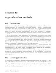
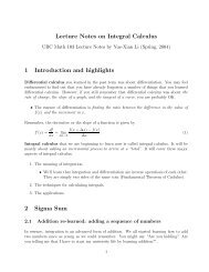
Math 103 Notes Chapter 10Now as T → ∞, we haveI T =[−Te −kT − e−kT+ 1 ].k kTe −kT → 0, e −kT → 0so that¯t = lim I T = 1T →∞ k .Thus the mean or expected decay time is¯t = 1 k .10.5 Discrete versus continuous probabilityIn an earlier chapter, we compared the treatment of two types of mass distributions. We firstexplored a set of discrete masses strung along a “thin wire”. Later, we considered a single “bar”with a continuous distribution of density along its length. In the first case, there was an unambiguousmeaning to the concept of “mass at a point”. In the second case, we could assign a mass to somesection of the bar between, say x = a and x = b. (To do so we had to integrate the mass density onthe interval a ≤ x ≤ b.) In the first case, we talked about the mass of the objects, whereas in thelatter case, we were interested in the idea of density (mass per unit distance: Note that the unitsof mass density are not the same as the units of mass.)The same dichotomy exists in the topic of probability. In an earlier chapter, we were concernedwith the probability of discrete events whose outcome belongs to some finite set of possibilities (e.g.Head or Tail for a coin toss, allele A or a in genetics). But many random processes lead to aninfinite, continuous set of possible outcomes. We need the notion of continuous probability to dealwith such cases. In continuous probability, we consider the probability density - analogous to massdensity. We can assign a probability to some range of values of the outcome between x = a andx = b. (To do so we have to integrate the probability density on the interval a ≤ x ≤ b.)The examples below provide some further insight to the connection between continuous anddiscrete probability. In particular, we will see that one can arrive at the idea of probability densityby refining a set of measurements and making the appropriate scaling. We explore this connectionin more detail below.10.5.1 Example: Student heightsSuppose we measure the heights of all UBC students. This would produce about 30,000 datavalues. We could make a graph and show how these heights are distributed. For example, we couldsubdivide the student body into those students between 0 and 1.5m, and those between 1.5 and 3meters. Our bar graph would contain two bars, with the number of students in each height categoryrepresented by the heights of the bars, as shown in Figure 10.3(a).Suppose we want to keep more detail. We could divide the population into smaller groups byshrinking the size of the interval or “bin” into which height is subdivided. (An example is shownv.2005.1 - January 5, 2009 10

Math 103 Notes Chapter 10p(h)p(h)p(h)∆ hh∆ hhhFigure 10.3: Refining a histogram by increasing the number of bins leads (eventually) to the ideaof a continuous probability density.in Figure 10.3(b)). Here, by a “bin” we mean a little interval of width ∆h where h is height, i.e. aheight interval. For example, we could keep track of the heights in increments of 50 cm. If we wereto plot the number of students in each height category, then as the size of the bins gets smaller,so would the height of the bar: there would be fewer students in each category if we increase thenumber of categories.To keep the bar height from shrinking, we might reorganize the data slightly. Instead of plottingthe number of students in each bin, we might plotnumber of students in bin.∆hIf we do this, then both numerator and denominator decrease as the size of the bins is made smaller,so that the shape of the distribution is preserved (i.e. it does not get flatter).We observe that in this case, the number of students in a given height category is representedby the area of the bar corresponding to that category:( )number of students in binArea of bin = ∆h= number of students in bin.∆hThe important point to consider is that the height of each bar in the plot represents the number ofstudents per unit height.This type of plot is precisely what leads us to the idea of a density distribution. As ∆h shrinks,we get a continuous graph. If we “normalize”, i.e. divide by the total area under the graph, we geta probability density, p(h) for the height of the population. As noted, p(h) represents the fractionof students per unit height whose height is h. It is thus a density, and has the appropriate units.More generally,p(x) ∆xrepresents the fraction of individuals whose height is in the range x ≤ h ≤ x + ∆x.10.5.2 Examples: Age dependent mortalityLet p(a) be a probability density for the probability of mortality of a female Canadian non-smoker atage a, where 0 ≤ a ≤ 120. (We have chosen an upper endpoint of age 120 since practically no Canav.2005.1- January 5, 2009 11

Math 103 Notes Chapter 10dian female lives past this age at present.) Let F(a) be the cumulative distribution correspondingto this probability density.(a) What is the probability of dying by age a?(b) What is the probability of surviving to age a?(c) Suppose that we are told that F(75) = 0.8 and that F(80) differs from F(75) by 0.11. Whatis the probability of surviving to age 80? Which is larger, F(75) or F(80)?(d) Use the information in part (c) to estimate the probability of dying between the ages of 75and 80 years old. Further, estimate p(80) from this information.Solution(a) The probability of dying by age a is the same as the probability of dying any time up to agea, i.e. it isF(a) =∫ a0p(s) ds,i.e. it is the cumulative distribution for this probability density. That, precisely, is the interpretationof the cumulative function.(b) The probability of surviving to age a is the same as the probability of not dying before agea. By the elementary properties of probability discussed in the previous chapter, this is1 − F(a).(c) From the properties of probability, we know that the cumulative distribution is an increasingfunction, and thus it must be true that F(80) > F(75). Then F(80) = F(75) + 0.11 = 0.8 + 0.11 =0.91. Thus the probability of surviving to age 80 is 1-0.91=0.09. This means that 9% of thepopulation will make it to their 80’th birthday, according to this analysis.(d) The probability of dying between the ages of 75 and 80 years old is exactly∫ 8075p(x) dx.However, we can also state this in terms of the cumulative function, since∫ 8075p(x) dx =∫ 800p(x) dx −∫ 750p(x) dx = F(80) − F(75) = 0.11Thus the probability of death between the ages of 75 and 80 is 0.11.To estimate p(80), we use the connection between the probability density and the cumulativedistribution:p(x) = F ′ (x).Then it is approximately true thatp(x) ≈F(x) − F(x − ∆x).∆xv.2005.1 - January 5, 2009 12

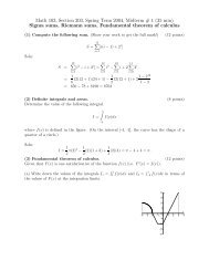
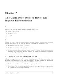
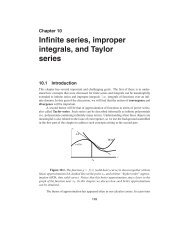
Math 103 Notes Chapter 10(Recall the definition of the derivative - the limit of the slope of the secant line as the widthincrements ∆x approach 0.)Thusp(80) ≈F(80) − F(75)5= 0.115= 0.022 per year10.5.3 Example: Raindrop size distributionDuring a Vancouver rainstorm, the density function which describes the radii of raindrops is constantover the range 0 ≤ r ≤ 4 (where r is measured in mm) and zero for larger r.(a) What is the density function p(r)?(b) What is the cumulative distribution F(r)?(c) In terms of the volume, what is the cumulative distribution F(V )?(d) In terms of the volume, what is the density function p(V )?(e) What is the average volume of a raindrop?SolutionThis problem is challenging because one may be tempted to think that the uniform distribution ofdrop radii should give a uniform distribution of drop volumes. This is not the case, as the followingargument shows! The sequence of steps is illustrated in Figure 10.4.p(r)F(r)r4 4rp(V)F(V)VVFigure 10.4: Probability densities for raindrop radius and raindrop volume (left panels) and for thecumulative distributions (right) of each.v.2005.1 - January 5, 2009 13

Math 103 Notes Chapter 10(a) The density function is p(r) = 1 0 ≤ r ≤ 4. This means that the probability per unit radius4of finding a drop of size r is the same for all radii in 0 ≤ r ≤ 4. Some of these drops will correspondto small volumes, and others to very large volumes. We will see that the probability per unit volumeof finding a drop of given volume will be quite different.(b) The cumulative distribution function isF(r) =∫ r014 ds = r 4 0 ≤ r ≤ 4.(c) The cumulative distribution function is proportional to the radius of the drop. We use theconnection between radii and volume of spheres to rewrite that function in terms of the volume ofthe drop: SinceV = 4 3 πr3we haveand sor =F(V ) = r 4 = 1 4( ) 1/3 3V 1/34π( ) 1/3 3V 1/3 .4πWe find the range of values of V by substituting r = 0, 4 into the equation V = 4 3 πr3 , to getV = 0,43 π43 . Therefore the interval is 0 ≤ V ≤ 4 3 π43 = (256/3)π.(d) We now use the connection between the probability density and the cumulative distribution,namely that p is the derivative of F. Now that the variable has been converted to volume, thatderivative is a little more “interesting”:p(V ) = F ′ (V )Therefore,p(V ) = 1 4( ) 1/3 3 14π 3 V −2/3 .Thus the probability per unit volume of finding a drop of volume V in 0 ≤ V ≤ 4 3 π43 is not at alluniform. This results from the fact that the differential quantity dr behaves very differently fromdV , and reinforces the fact that we are dealing with density, not with a probability per se. We notethat this distribution has smaller values at larger values of V .(e) The range of values of V is0 ≤ V ≤ 4 3 π43 = 256π3v.2005.1 - January 5, 2009 14

Math 103 Notes Chapter 10and therefore the mean volume is¯V =∫ 256π/30= 112= 112= 112= 116V p(V )dV( ) 1/3 ∫ 3 256π/3V · V −2/3 dV4π 0( ) 1/3 ∫ 3 256π/3V 1/3 dV4π 0( ) 1/3∣ 3 3 ∣∣∣256π/34π 4 V 4/3 0( ) 1/3 ( ) 4/33 256π4π 3= 64π3 ≈ 67mm3 .10.6 Moments of a probability distributionWe are now familiar with some of the properties of probability distributions. On this page we willintroduce a set of numbers that describe various properties of such distributions. Some of thesehave already been encountered in our previous discussion, but now we will see that these fit into apattern of quantities called moments of the distribution.MomentsLet f(x) be any function which is defined and positive on an interval [a, b]. We might refer to thefunction as a distribution, whether or not we consider it to be a probability density distribution.Then we will define the following moments of this function:zero’th moment M 0 =first moment M 1 =second moment M 2 =∫ ba∫ ba∫ baf(x) dxx f(x) dxx 2 f(x) dxn’th moment M n =.∫ bax n f(x) dx.Observe that moments of any order are defined by integrating the distribution f(x) with asuitable power of x over the interval [a, b]. However, in practice we will see that usually momentsv.2005.1 - January 5, 2009 15

Math 103 Notes Chapter 10up to the second are usefully employed to describe common attributes of a distribution.10.6.1 Moments of a probability density distributionIn the particular case that the distribution is a probability density, p(x), defined on the intervala ≤ x ≤ b, we have already established the following :M 0 =∫ bap(x) dx = 1(This follows from the basic property of a probability density.) ThusThe zero’th moment of any probability density is 1.FurtherM 1 =∫ bax p(x) dx = ¯x = µ.That is,The first moment of a probability density is the same as the mean (i.e. expected value) of thatprobability density.So far, we have used the symbol ¯x to represent the mean or average value of x but often thesymbol µ is also used to denote the mean.The second moment, of a probability density also has a useful interpretation. From abovedefinitions, the second moment of p(x) over the interval a ≤ x ≤ b isM 2 =∫ bax 2 p(x) dxWe will shortly see that the second moment helps describe the way that density is distributed aboutthe mean. For this purpose, we must describe the notion of variance or standard deviation.Variance and standard deviationTwo kids of approximately the same size can balance on a teeter-totter by sitting very close to thepoint at which the beam pivots. They can also achieve a balance by sitting at the very ends of thebeam, equally far away. In both cases, the center of mass of the distribution is at the same place:precisely at the pivot point. However, the mass is distributed very differently in these two cases.In the first case, the mass is clustered close to the center, whereas in the second, it is distributedfurther away. We may want to be able to describe this distinction, and we could do so by consideringhigher moments of the mass distribution.Similarly, if we want to describe how a probability density distribution is distributed about itsmean, we consider moments higher than the first. We use the idea of the variance to describewhether the distribution is clustered close to its mean, or spread out over a great distance from themean.v.2005.1 - January 5, 2009 16

Math 103 Notes Chapter 10VarianceThe variance is defined as the average value of the quantity (distance from mean) 2 , where theaverage is taken over the whole distribution. (The reason for the square is that we would not likevalues to the left and right of the mean to cancel out.)For discrete probability with mean, µ we define variance byV = ∑ (x i − µ) 2 p iFor a continuous probability density, with mean µ, we define the variance byV =∫ ba(x − µ) 2 p(x) dxThe standard deviationThe standard deviation is defined asσ = √ VLet us see what this implies about the connection between the variance and the moments of thedistribution.Relationship of variance to second moment¿From the equation for variance we calculate thatV =∫ baExpanding the integral leads to:(x − µ) 2 p(x) dx =∫ ba(x 2 − 2µx + µ 2 ) p(x) dx.V ==∫ ba∫ bax 2 p(x)dx −∫ bx 2 p(x)dx − 2µa∫ b2µx p(x) dx +a∫ bx p(x) dx + µ 2 ∫ baµ 2 p(x) dxap(x) dx.We recognize the integrals in the above expression, since they are simply moments of the probabilitydistribution. Plugging in these facts, we arrive atv.2005.1 - January 5, 2009 17

Math 103 Notes Chapter 10ThusV = M 2 − 2µ µ + µ 2V = M 2 − µ 2Thus the variance is clearly related to the second moment and to the mean of the distribution.Relationship of variance to second moment¿From the definitions given above, we find thatσ = √ V = √ M 2 − µ 210.6.2 ExampleConsider the continuous distribution, in which the probability is constant, p(x) = C, for values of xin the interval [a, b] and zero for values outside this interval. Such a distribution is called a uniformdistribution. (It has the shape of a rectangular band of height C and base (b − a).) It is easy tosee that the value of the constant C should be 1/(b − a) so that the area under this rectangularband will be 1, in keeping with the property of a probability distribution. Thus the equation of thisprobability is p(x) = 1 . We compute the first moments of this probability densityb − aM 0 =∫ bap(x)dx = 1b − a∫ ba1 dx = 1.(This was already known, since we have determined that the zeroth moment of any probabilitydensity is 1.) We also find thatM 1 =∫ bx p(x) dx = 1 x dxb − a a= 1x 2bb − a 2 ∣ = b2 − a 22(b − a) .This last expression can be simplified by factoring, leading toaµ = M 1 =a(b − a)(b + a)2(b − a)∫ b= b + a2Thus we have found that the mean µ is in the center of the interval [a, b], as expected. The medianwould be at the same place by a simple symmetry argument: half the area is to the left and halfthe area is to the right of this point.v.2005.1 - January 5, 2009 18

Math 103 Notes Chapter 10To find the variance we might first calculate the second moment,M 2 = x 2 p(x) dx = 1 ∫ bx 2 dxab − a aIt can be shown by simple integration that this yields the result∫ bwhich can be simplified toM 2 = b3 − a 33(b − a) ,M 2 = (b − a)(b2 + ab + a 2 )3(b − a)= b2 + ab + a 2.3We would then compute the varianceAfter simplification, we getThe standard deviation is thenV = M 2 − µ 2 = b2 + ab + a 2−3V = b2 − 2ab + a 212σ ==(b − a)2 √ 3 .(b − a)2.12(b + a)2.4v.2005.1 - January 5, 2009 19