Passivity based control of port-controlled Hamiltonian systems
Passivity based control of port-controlled Hamiltonian systems
Passivity based control of port-controlled Hamiltonian systems

Create successful ePaper yourself
Turn your PDF publications into a flip-book with our unique Google optimized e-Paper software.
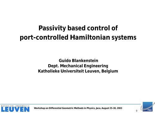
<strong>Passivity</strong> <strong>based</strong> <strong>control</strong> <strong>of</strong><strong>port</strong>-<strong>control</strong>led <strong>Hamiltonian</strong> <strong>systems</strong>Guido BlankensteinDept. Mechanical EngineeringKatholieke Universiteit Leuven, BelgiumWorkshop on Differential Geometric Methods in Physics, Jaca, August 25-30, 20030
2. Port-<strong>control</strong>led <strong>Hamiltonian</strong> <strong>systems</strong>Port-<strong>control</strong>led <strong>Hamiltonian</strong> <strong>systems</strong> have the general form( ) (−ẋ∂H∂xF (x) + E(x)(x))= 0 (1)f ext e extwhere H(x) is the energy function, and f ext , e ext are dual externalvariables, with 〈e ext |f ext 〉 power.HereD = {(X, f ext , α, e ext ) ∈ T X ⊕ V ⊕ T ∗ X ⊕ V |( ) ( )X(x)α(x)F (x) + E(x) = 0} (2)f ext e extis a generalized Dirac structure, i.e., rank[F (x) E(x)] = dim X +dim Vand E(x)F T (x) + F (x)E T (x) = 0.Workshop on Differential Geometric Methods in Physics, Jaca, August 25-30, 20032
The system is energy conserving:ddt H(x(t)) = 〈e ext(t)|f ext (t)〉 (3)If the system contains dissipative elements (e.g. dampers, resistors),thenE(x)F T (x) + F (x)E T (x) ≤ 0 (4)and the power balance changes intoddt H(x(t)) ≤ 〈e ext(t)|f ext (t)〉 (5)Examples are electrical RLC circuits, mechanical multi-body <strong>systems</strong>,mechanical <strong>systems</strong> with kinematic constraints, electromechanicalsystem, physical network models, etc.Workshop on Differential Geometric Methods in Physics, Jaca, August 25-30, 20033
A common class <strong>of</strong> <strong>port</strong>-<strong>control</strong>led <strong>Hamiltonian</strong> <strong>systems</strong> is given by( ) ( ) ( ) ( I 0 −ẋ J(x) − R(x) g(x) ∂H+0 I y −g T ∂x (x))= 0 (6)(x) 0 uyieldingExamples includeẋ = (J(x) − R(x)) ∂H (x) + g(x)u∂x (7a)y = g T (x) ∂H∂x (x)(7b)• electrical circuits with independent elements( ) 0 I• mechanical <strong>systems</strong>: x = (q, p) and J = J =−I 0• (non-holonomic) kinematically constrained mechanical <strong>systems</strong>:x = (q, p 1 ), and J the restriction <strong>of</strong> J to the constraintmanifold X constraint ⊂ T ∗ X .Workshop on Differential Geometric Methods in Physics, Jaca, August 25-30, 20034
3. <strong>Passivity</strong> <strong>based</strong> <strong>control</strong>Port-<strong>control</strong>led <strong>Hamiltonian</strong> <strong>systems</strong> satisfy the power balance:ddt H(x(t)) = uT (t)y(t) − ∂H T(x(t))R(x(t)) ∂H (x(t)) (8)∂x∂xwhich upon integration yields the energy balance∫ tH(x(t)) − H(x(0)) = u T (τ)y(τ)dτ −} {{ } 0} {{ }stored energysupplied energy∫ tT∂H(x(τ))R(x(τ)) ∂H0 ∂x∂x (x(τ))dτ} {{ }≥0, dissipated energy(9)If H is non-negative, we say the system is passive. For u T y ≡ 0,Ḣ ≤ 0 and consequently ¯x = argmin H(x) is a stable equilibrium.Workshop on Differential Geometric Methods in Physics, Jaca, August 25-30, 20035
To stabilize a desired equilibrium point x ⋆ ≠ ¯x, find a <strong>control</strong>leru = β(x) + v such that the closed loop dynamics satisfyH s (x(t)) − H s (x(0)) =∫ t0v T (τ)y s (τ)dτ − R s (t)} {{ }≥0(10)with x ⋆ = argmin H s (x). The closed loop system is passive, andhence x ⋆ is a stable equilibrium.This is called passivity <strong>based</strong> <strong>control</strong>.In this presentation we discuss two PBC methods:• <strong>control</strong> by interconnection• interconnection and damping assigmentWorkshop on Differential Geometric Methods in Physics, Jaca, August 25-30, 20036
4. Control by interconnectionApply the interconnectivity <strong>of</strong> <strong>port</strong>-<strong>Hamiltonian</strong> <strong>systems</strong> for <strong>control</strong>purposes.v + u yPlant−y_cControlleru_cControl by interconnection.Workshop on Differential Geometric Methods in Physics, Jaca, August 25-30, 20037
Port-<strong>Hamiltonian</strong> plant system:Controller system:ẋ = (J(x) − R(x)) ∂H (x) + g(x)u∂x (11a)y = g T (x) ∂H∂x (x)˙ξ = (J c (ξ) − R c (ξ)) ∂H c∂ξ (ξ) + g c(ξ)u cy c = g T c (ξ) ∂H c∂ξ (ξ)(11b)(12a)(12b)Standard feedback interconnection:u = −y c + v, u c = y (13)Workshop on Differential Geometric Methods in Physics, Jaca, August 25-30, 20038
The closed loop system has the form(ẋ )= [( J(x) −g(x)g T )c (ξ)˙ξ g c (ξ)g T (x) J c (ξ)( ) g(x)+ v0y = ( g T (x)0 ) ( ∂H∂x (x))∂H c∂ξ (ξ)( ) (R(x) 0 ]∂H∂x−(x))0 R c (ξ) ∂H c∂ξ (ξ)(14a)(14b)which is again <strong>port</strong>-<strong>Hamiltonian</strong> with closed loop energy functionH cl (x, ξ) = H(x) + H c (ξ) (15)Now, suppose we can eliminate the <strong>control</strong>ler variables ξ by findingconstant functions C(x, ξ) = ξ − C(x), then the closed loop energy isH cl (x) = H(x) + H c (C(x)) (16)The x-dynamics is <strong>port</strong>-<strong>Hamiltonian</strong> with shaped energy function.Workshop on Differential Geometric Methods in Physics, Jaca, August 25-30, 20039
C(x, ξ) = ξ − C(x) are constant if (assume v = 0)( ( −∂C∂x (x) I) J(x) − R(x) −g(x)gc T )(ξ)g c (ξ)g T = 0 (17)(x) J c (ξ) − R c (ξ)Lemma: (17) holds iffT∂C(x)(x)J(x) ∂C(x)∂x∂x (x) = J c(ξ) (18a)R(x) ∂C(x) (x) = 0 (18b)∂xR c (ξ) = 0(18c)T∂C(x)(x)J(x) = g c (ξ)g T (x)∂x(18d)In fact, the functions ξ − C(x) are Casimirs.Workshop on Differential Geometric Methods in Physics, Jaca, August 25-30, 200310
Reduced dynamics on a multi-level set L = {(x, ξ)|ξ−C(x) = const.}ẋ = (J(x) − R(x)) ∂H∂x (x) − g(x)gT c (ξ) ∂H c∂ξ (ξ)= [ J(x) − R(x) ]( ∂H∂x= [ J(x) − R(x) ] ∂H s∂x (x)with shaped energy function(x) +∂C(x)∂x∂H c∂ξ (ξ)) (19)H s (x) = H(x) + H c (C(x)) (20)Energy balancing <strong>control</strong>:H s (x(t)) = H(x(t)) +∫ t0u T c (τ)y c (τ)dτ = H(x(t)) −∫ t0u T (τ)y(τ)dτWorkshop on Differential Geometric Methods in Physics, Jaca, August 25-30, 200311
5. Control by interconnection – mechanical <strong>systems</strong>Mechanical system:( ( ˙q 0 In=ṗ)−I n −R(q)y = G T (q) ∂H∂p) ( ∂H∂q∂H∂p)( ) 0+ uG(q)(21a)(21b)Total energyH(q, p) = 1 2 pT M −1 (q)p + P (q) (22)Workshop on Differential Geometric Methods in Physics, Jaca, August 25-30, 200312
The functions ξ − C(q, p) are Casimirs iff∂CT ∂C∂q ∂p − ∂C T ∂C∂p ∂q = J c(ξ)R(q) ∂C∂p = 0R c (ξ) = 0(23a)(23b)(23c)T∂C∂p= 0,T∂C∂q= g c (ξ)G T (q) (23d)Equivalenlty,J c = 0,∂C∂p = 0,gT c (ξ)G(q) = ∂C (q) (24)∂qChoose g c (ξ) = I m , then Casimirs exist iff G is integrable:∂G ik∂q j(q) = ∂G jk∂q i(q) (25)Workshop on Differential Geometric Methods in Physics, Jaca, August 25-30, 200313
E.g. assume full actuation: G(q) = I nCasimirs ξ − C(q, p) = ξ − q (26)Closed loop dynamics reduced on multi-level set( ( ) ˙q 0 In=ṗ)( )∂H s∂q−I n −R(q)∂H s∂p(27)withH s (q, p) = H(q, p) + H c (q)= 1 2 pT M −1 (q)p + [ P (q) + H c (q) ] (28)Hence, this method amounts to potential energy shaping.Workshop on Differential Geometric Methods in Physics, Jaca, August 25-30, 200314
6. Example: inverted pendulumEuler-Lagrange equations: ¨q + sin q + d ˙q = uPort-<strong>control</strong>led <strong>Hamiltonian</strong> model:( ( ˙q 0 1=ṗ)−1 −dy = ∂H∂p = ˙q) ( ∂H∂q∂H∂p)( 0+ u1)(29a)(29b)with H(q, p) = 1 2 p2 + (1 − cos q).Problem: Stabilize upright position <strong>of</strong> the pendulum, at q = π.The Casimir is given by ξ−C(q, p) = ξ−q. Hence, the simplest choiceis to takeH c (ξ) = cos ξ + 1 2 κ(ξ − π)2 (30)Workshop on Differential Geometric Methods in Physics, Jaca, August 25-30, 200315
Then the energy <strong>of</strong> the closed loop isH s (q, p) = H(q, p) + H c (q)= 1 2 p2 + (1 − cos q) + cos q + 1 2 κ(q − π)2 (31)= 1 2 p2 + 1 2 κ(q − π)2 + 1which has a strict minimum in (q, p) = (π, 0). Hence, the uprightposition is asymptotically stable.The <strong>control</strong>ler system (J c (ξ) = R c (ξ) = 0, g c (ξ) = 1) is:˙ξ = u c (= y = ˙q) (32a)y c = ∂H c(ξ) = − sin ξ + κ(ξ − π) (= −u) (32b)∂ξwhich represents a potential torque consisting <strong>of</strong>• gravity compensation• virtual spring, with stiffness κ and equilibrium at q = πWorkshop on Differential Geometric Methods in Physics, Jaca, August 25-30, 200316
7. Drawbacks <strong>of</strong> <strong>control</strong> by interconnectionTwo possible drawbacks <strong>of</strong> the method:• doesn’t work in the presence <strong>of</strong> pervasive dissipation• restricted to potential energy shaping in case <strong>of</strong> mechanical<strong>systems</strong>Workshop on Differential Geometric Methods in Physics, Jaca, August 25-30, 200317
7.1. Drawback: pervasive dissipationRecall energy balancing:H s (x(t)) = H(x(t)) −∫ t0u T (τ)y(τ)dτ (33)Differentiate w.r.t. time to get ∂(Hs−H)∂x(x(t))ẋ(t) = −u T (t)y(t)At the desired equilibrium, ẋ = 0, this yields0 = −(u ⋆ ) T y ⋆ (34)Hence, the power extracted from the <strong>control</strong>ler at the equilibriumshould be zero.For mechanical <strong>systems</strong> this is ok: y ⋆ = ˙q| q=q ⋆ = 0However, for some electrical or electromechanical <strong>systems</strong> this conditionis not always satisfied, e.g. parallel RLC circuit.Workshop on Differential Geometric Methods in Physics, Jaca, August 25-30, 200318
7.2. Drawback: only potential energy shapingUnderactuated mechanical <strong>systems</strong> generally need kinetic energyshaping, next to potential energy shaping.180 - q 2uq 1Inverted pendulum on a cart.Workshop on Differential Geometric Methods in Physics, Jaca, August 25-30, 200319
8. Interconnection and damping assignment (IDA-PBC)Port-<strong>Hamiltonian</strong> plant system:ẋ = (J(x) − R(x)) ∂H (x) + g(x)u∂x (35a)y = g T (x) ∂H∂x (x)(35b)Look for a static state feedback <strong>control</strong> law u = β(x) + v such thatthe closed loop system becomesẋ = (J s (x) − R s (x)) ∂H s(x) + g(x)v∂x (36a)y s = g T (x) ∂H s∂x (x)(36b)with shaped interconnection structure J s , damping structure R s , andenergy function H s .Workshop on Differential Geometric Methods in Physics, Jaca, August 25-30, 200320
Equating open loop and closed loop gives(J(x) − R(x)) ∂H∂x (x) + g(x)β(x) = (J s(x) − R s (x)) ∂H s(x) (37)∂xwhich which is equivalent to (matching conditions)g ⊥ (x) [ (J s (x) − R s (x)) ∂H s(x) − (J(x) − R(x))∂H∂x ∂x (x)] = 0 (38)where g ⊥ is a left annihilator <strong>of</strong> g, i.e., g ⊥ (x)g(x) = 0.Eq. (38) is a set <strong>of</strong> non-linear PDEs in J s , R s and H s . If a solutionexists, thenβ(x) = (g T (x)g(x)) −1 g T (x) [ (J s (x)−R s (x)) ∂H s∂x (x)−(J(x)−R(x))∂H ∂x (x)]Workshop on Differential Geometric Methods in Physics, Jaca, August 25-30, 200321
9. IDA-PBC for mechanical <strong>systems</strong>Mechanical system:( ( ˙q 0 In=ṗ)−I n −R(q)y = G T (q) ∂H∂p) ( ∂H∂q∂H∂p)( ) 0+ uG(q)(39a)(39b)with total energy H(q, p) = 1 2 pT M −1 (q)p + P (q)Find a state feedback law u = β(q, p) such that( ˙qṗ)= [ ( 0 0J s (q, p) −0 R s (q)) ]( ∂Hs∂q∂H s∂p)(40)with shaped energy H s (q, p) = 1 2 pT Ms−1 (q)p + P s (q)Workshop on Differential Geometric Methods in Physics, Jaca, August 25-30, 200322
Since ˙q = M −1 (q)p is an non-actuated coordinate, J s has the form(0 MJ s (q, p) =−1 )(q)M s (q)−M s (q)M −1 (q) Js 22(41)(q, p)Equating open loop and closed loop yields( ) ( )∂H ( 0 In ∂q 0+ β =−I n −R M −1 p G)[ ( 0 0J s −) ( )]∂Hs∂q0 R s pM −1sThe matching conditions areG ⊥ (q) [ ∂H∂q (q, p) + R(q)M −1 (q)p − M s (q)M −1 (q) ∂H s(q, p)∂q+ ( Js22 (q, p) − R s (q) ) Ms −1 (q)p ] = 0 (42)Workshop on Differential Geometric Methods in Physics, Jaca, August 25-30, 200323
Collecting terms quadratic, linear and independent <strong>of</strong> p yields:G ⊥[ ∂ q ( 1 2 pT M −1 p)−M s M −1 ∂ q ( 1 2 pT Ms −1 p)+(Js22 ) q,p Ms −1 p ] = 0 (43)which is a non-linear PDE in M s and J 22s ,G ⊥[ RM −1 p + ( (Js22 ) q )− R s M−1s p ] = 0 (44)which is a linear PDE in R s , andwhich is a linear PDE in P s .G ⊥[ ∂ q P − M s M −1 ∂ q P s]= 0 (45)Workshop on Differential Geometric Methods in Physics, Jaca, August 25-30, 200324
10. Example: inverted pendulum on a cartConfiguration q = (q 1 , q 2 ) = (position cart, angle pendulum). Onlyactuation <strong>of</strong> the first coordinate, hence( 1G(q) = , G0)⊥ (q) = ( 0 1 ) (46)Potential energy <strong>of</strong> the pendulum: P (q 1 , q 2 ) = 1 − cos q 2Try to stabilize the upright position <strong>of</strong> the pendulum, at q 2 = π, bypotential energy shaping, i.e., M s (q) = M(q):( )[ ( ) ( )0 ∂q1 P 0 1 − s ]= 0 (47)sin q 2 ∂ q2 P sThis has solutionsP s (q 1 , q 2 ) = − cos q 2 + Φ(q 1 ) (48)which do not have a minimum in q 2 = π.Workshop on Differential Geometric Methods in Physics, Jaca, August 25-30, 200325
11. Some remarks on IDA-PBC• Sometimes the non-linear PDEs can be written as a set <strong>of</strong> nonlinearODEs.• The non-linear PDEs can be written as a set <strong>of</strong> quasi-linearPDEs (λ-method).• There exists an explicit choice <strong>of</strong> Js22 under which the closedloop system is Euler-Lagrangian (Controlled Lagrangians Method).• Extension to dynamic feedback (to avoid velocity measurement).• Universal stabilizing property!• Extension to <strong>port</strong>-<strong>control</strong>led <strong>Hamiltonian</strong> <strong>systems</strong> with constraints(e.g. mechanical <strong>systems</strong> with kinematic constraints).Workshop on Differential Geometric Methods in Physics, Jaca, August 25-30, 200326
12. Summary• Port-<strong>control</strong>led <strong>Hamiltonian</strong> system: dynamical system w.r.t.(dissipative 1 ) Dirac structure• <strong>Passivity</strong> <strong>based</strong> <strong>control</strong>: energy shaping to stabilize a desiredequilibrium• Control by interconnection: feedback loop with PCH <strong>control</strong>ler,dynamics restricted to Casimir level set• Mechanical <strong>systems</strong>: only potential energy shaping• Interconnection and damping assignment (IDA-PBC): static statefeedback• (Underactuated) mechanical <strong>systems</strong>: total energy shaping• http://www.geoplex.cc1 non-canonicalWorkshop on Differential Geometric Methods in Physics, Jaca, August 25-30, 200327