Chapter 47: Theory and Analysis of Structures - Free

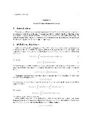
47Theory and Analysisof StructuresJ.Y. Richard LiewNational University of SingaporeN.E. ShanmugamNational University of Singapore47.1 Fundamental PrinciplesBoundary Conditions • Loads and Reactions • Principle ofSuperposition47.2 BeamsRelation between Load, Shear Force, and Bending Moment •Shear Force and Bending Moment Diagrams • Fixed-EndBeams • Continuous Beams • Beam Deflection • Curved Beams47.3 TrussesMethod of Joints • Method of Sections • Compound Trusses47.4 FramesSlope Deflection Method • Frame Analysis Using SlopeDeflection Method • Moment Distribution Method • Methodof Consistent Deformations47.5 PlatesBending of Thin Plates • Boundary Conditions • Bending ofRectangular Plates • Bending of Circular Plates • Strain Energyof Simple Plates • Plates of Various Shapes and BoundaryConditions • Orthotropic Plates47.6 ShellsStress Resultants in Shell Element • Shells of Revolution •Spherical Dome • Conical Shells • Shells of RevolutionSubjected to Unsymmetrical Loading • Cylindrical Shells •Symmetrically Loaded Circular Cylindrical Shells47.7 Influence Lines .Influence Lines for Shear in Simple Beams • Influence Lines forBending Moment in Simple Beams • Influence Lines forTrusses • Qualitative Influence Lines • Influence Lines forContinuous Beams47.8 Energy MethodsStrain Energy Due to Uniaxial Stress • Strain Energy inBending • Strain Energy in Shear • The Energy Relations inStructural Analysis • Unit Load Method47.9 Matrix MethodsFlexibility Method • Stiffness Method • Element StiffnessMatrix • Structure Stiffness Matrix • Loading between Nodes •Semirigid End Connection© 2003 by CRC Press LLC

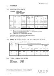
47-2 The Civil Engineering Handbook, Second Edition47.1 Fundamental Principles47.10 Finite Element MethodBasic Principle • Elastic Formulation • Plane Stress • PlaneStrain • Choice of Element Shapes and Sizes • Choice ofDisplacement Function • Nodal Degrees of Freedom •Isoparametric Elements • Isoparametric Families of Elements •Element Shape Functions • Formulation of Stiffness Matrix •Plates Subjected to In-Plane Forces • Beam Element • PlateElement47.11 Inelastic AnalysisAn Overall View • Ductility • Redistribution of Forces •Concept of Plastic Hinge • Plastic Moment Capacity • Theoryof Plastic Analysis • Equilibrium Method • MechanismMethod • Analysis Aids for Gable Frames • Grillages •Vierendeel Girders • Hinge-by-Hinge Analysis47.12 Stability of StructuresStability Analysis Methods • Column Stability • Stability ofBeam-Columns • Slope Deflection Equations • Second-OrderElastic Analysis • Modifications to Account for Plastic HingeEffects • Modification for End Connections • Second-OrderRefined Plastic Hinge Analysis • Second-Order Spread ofPlasticity Analysis • Three-Dimensional Frame Element •Buckling of Thin Plates • Buckling of Shells47.13 Dynamic AnalysisEquation of Motion • Free Vibration • Forced Vibration •Response to Suddenly Applied Load • Response to Time-Varying Loads • Multiple Degree Systems • Distributed MassSystems • Portal Frames • Damping • Numerical AnalysisThe main purpose of structural analysis is to determine forces and deformations of the structure due toapplied loads. Structural design involves form finding, determination of loadings, and proportioning ofstructural members and components in such a way that the assembled structure is capable of supportingthe loads within the design limit states. An analytical model is an idealization of the actual structure.The structural model should relate the actual behavior to material properties, structural details, loading,and boundary conditions as accurately as is practicable.Structures often appear in three-dimensional forms. For structures that have a regular layout and arerectangular in shape, subject to symmetric loads, it is possible to idealize them into two-dimensionalframes arranged in orthogonal directions. A structure is said to be two-dimensional or planar if all themembers lie in the same plane. Joints in a structure are those points where two or more members areconnected. Beams are members subjected to loading acting transversely to their longitudinal axis andcreating flexural bending only. Ties are members that are subjected to axial tension only, while struts(columns or posts) are members subjected to axial compression only. A truss is a structural systemconsisting of members that are designed to resist only axial forces. A structural system in which jointsare capable of transferring end moments is called a frame. Members in this system are assumed to becapable of resisting bending moments, axial force, and shear force.Boundary ConditionsA hinge or pinned joint does not allow translational movements (Fig. 47.1a). It is assumed to be frictionlessand to allow rotation of a member with respect to the others. A roller permits the attached structuralpart to rotate freely with respect to the rigid surface and to translate freely in the direction parallel tothe surface (Fig. 47.1b). Translational movement in any other direction is not allowed. A fixed support(Fig. 47.1c) does not allow rotation or translation in any direction. A rotational spring provides some© 2003 by CRC Press LLC

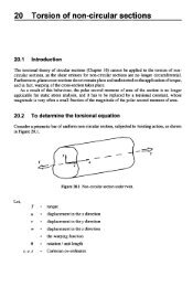
Theory and Analysis of Structures 47-3(a) Hinge support(b) Roller support(c) Fixed support(d) Rotational spring(e) Translational springFIGURE 47.1 Various boundary conditions.rotational restraint but does not provide any translational restraint (Fig. 47.1d). A translational springcan provide partial restraints along the direction of deformation (Fig. 47.1e).Loads and ReactionsLoads that are of constant magnitude and remain in the original position are called permanent loads.They are also referred to as dead loads, which may include the self weight of the structure and otherloads, such as walls, floors, roof, plumbing, and fixtures that are permanently attached to the structure.Loads that may change in position and magnitude are called variable loads. They are commonly referredto as live or imposed loads, which may include those caused by construction operations, wind, rain,earthquakes, snow, blasts, and temperature changes, in addition to those that are movable, such asfurniture and warehouse materials.Ponding loads are due to water or snow on a flat roof that accumulates faster than it runs off. Windloads act as pressures on windward surfaces and pressures or suctions on leeward surfaces. Impact loadsare caused by suddenly applied loads or by the vibration of moving or movable loads. They are usuallytaken as a fraction of the live loads. Earthquake loads are those forces caused by the acceleration of theground surface during an earthquake.A structure that is initially at rest and remains at rest when acted upon by applied loads is said to bein a state of equilibrium. The resultant of the external loads on the body and the supporting forces orreactions is zero. If a structure is to be in equilibrium under the action of a system of loads, it mustsatisfy the six static equilibrium equations:Â Fx = 0, Â Fy = 0, Â Fz= 0Â Mx = 0, Â My = 0, Â Mz= 0(47.1)The summation in these equations is for all the components of the forces (F) and of the moments(M) about each of the three axes x, y, and z. If a structure is subjected to forces that lie in one plane, sayx-y, the above equations are reduced to:Â Fx = 0, Â Fy = 0, Â Mz= 0(47.2)Consider a beam under the action of the applied loads, as shown in Fig. 47.2a. The reaction at supportB must act perpendicular to the surface on which the rollers are constrained to roll upon. The support© 2003 by CRC Press LLC

47-4 The Civil Engineering Handbook, Second Edition400 kNA5 mC60°5 mB30°(a) Applied load400 Sin 60° = 346.4 kNA x400 Cos 60° = 200 kN B xA yB yFIGURE 47.2 Beam in equilibrium.reactions and the applied loads, which are resolved in vertical and horizontal directions, are shown inFig. 47.2b.From geometry, it can be calculated that B y = 3B x 1. Equation (47.2) can be used to determine themagnitude of the support reactions. Taking moment about B givesfrom which10A y – 346.4 ¥ 5 = 0A y = 173.2 kNEquating the sum of vertical forces, SF y , to zero givesand hence we getTherefore173.2 + B y – 346.4 = 0B y = 173.2 kNEquilibrium in the horizontal direction, SF x = 0, givesand hence(b) Support reactionsB = B 3 = 100 kN.xyA x – 200 – 100 = 0A x = 300 kNThere are three unknown reaction components at a fixed end, two at a hinge, and one at a roller. If,for a particular structure, the total number of unknown reaction components equal the number ofequations available, the unknowns may be calculated from the equilibrium equations, and the structureis then said to be statically determinate externally. Should the number of unknowns be greater than thenumber of equations available, the structure is statically indeterminate externally; if less, it is unstableexternally. The ability of a structure to support adequately the loads applied to it is dependent not onlyon the number of reaction components but also on the arrangement of those components. It is possiblefor a structure to have as many or more reaction components than there are equations available and yetbe unstable. This condition is referred to as geometric instability.© 2003 by CRC Press LLC

Theory and Analysis of Structures 47-5Principle of SuperpositionThe principle states that if the structural behavior is linearly elastic, the forces acting on a structure maybe separated or divided into any convenient fashion and the structure analyzed for the separate cases.The final results can be obtained by adding up the individual results. This is applicable to the computationof structural responses such as moment, shear, deflection, etc.However, there are two situations where the principle of superposition cannot be applied. The firstcase is associated with instances where the geometry of the structure is appreciably altered under load.The second case is in situations where the structure is composed of a material in which the stress is notlinearly related to the strain.47.2 BeamsOne of the most common structural elements is a beam; it bends when subjected to loads actingtransversely to its centroidal axis or sometimes by loads acting both transversely and parallel to this axis.The discussions given in the following subsections are limited to straight beams in which the centroidalaxis is a straight line with a shear center coinciding with the centroid of the cross-section. It is alsoassumed that all the loads and reactions lie in a simple plane that also contains the centroidal axis of theflexural member and the principal axis of every cross-section. If these conditions are satisfied, the beamwill simply bend in the plane of loading without twisting.Relation between Load, Shear Force, and Bending MomentShear force at any transverse cross-section of a straight beam is the algebraic sum of the componentsacting transverse to the axis of the beam of all the loads and reactions applied to the portion of the beamon either side of the cross-section. Bending moment at any transverse cross-section of a straight beam isthe algebraic sum of the moments, taken about an axis passing through the centroid of the cross-section.The axis about which the moments are taken is, of course, normal to the plane of loading.When a beam is subjected to transverse loads, there exist certain relationships between load, shearforce, and bending moment. Let us consider the beam shown in Fig. 47.3 subjected to some arbitraryloading, p. Let S and M be the shear and bending moment, respectively, for any point m at a distance x,which is measured from A, being positive when measured to the right. Corresponding values of the shearand bending moment at point n at a differential distance dx to the right of m are S + dS and M + dM,respectively. It can be shown, neglecting the second order quantities, thatdSp =dx(47.3)andS =dMdx(47.4)p/unit lengthAxx C× × × ×C m n Ddxx DLBFIGURE 47.3 Beam under arbitrary loading.© 2003 by CRC Press LLC

47-6 The Civil Engineering Handbook, Second EditionEquation (47.3) shows that the rate of change of shear at any point is equal to the intensity of loadapplied to the beam at that point. Therefore, the difference in shear at two cross-sections C and D isX DS - S = pÚ dxDC(47.5)X cWe can write this in the same way for moment asMDxD- MC= S dxÚxC(47.6)Shear Force and Bending Moment DiagramsIn order to plot the shear force and bending moment diagrams, it is necessary to adopt a sign conventionfor these responses. A shear force is considered to be positive if it produces a clockwise moment abouta point in the free body on which it acts. A negative shear force produces a counterclockwise momentabout the point. The bending moment is taken as positive if it causes compression in the upper fibersof the beam and tension in the lower fiber. In other words, a sagging moment is positive and a hoggingmoment is negative. The construction of these diagrams is explained with an example given in Fig. 47.4.Section E of the beam is in equilibrium under the action of applied loads and internal forces actingat E, as shown in Fig. 47.5. There must be an internal vertical force and internal bending moment tomaintain equilibrium at section E. The vertical force or the moment can be obtained as the algebraicsum of all forces or the algebraic sum of the moment of all forces that lie on either side of section E.The shear on a cross-section an infinitesimal distance to the right of point A is +55, and therefore theshear diagram rises abruptly from zero to +55 at this point. In portion AC, since there is no additionalload, the shear remains +55 on any cross-section throughout this interval, and the diagram is a horizontal,as shown in Fig. 47.4. An infinitesimal distance to the left of C the shear is +55, but an infinitesimalx30 kN 4 kN/m 40 kNAC D E F3 4 6 8 955 kN30 m55+ 2511−343351265165B39 kN39FIGURE 47.4 Bending moment and shear force diagrams.A55 kN4 kN/mEC D3 m 4 m 6 mVCTFIGURE 47.5 Internal forces.© 2003 by CRC Press LLC

Theory and Analysis of Structures 47-7distance to the right of this point the concentrated load of magnitude 30 has caused the shear to bereduced to +25. Therefore, at point C, there is an abrupt change in the shear force from +55 to +25. Inthe same manner, the shear force diagram for portion CD of the beam remains a rectangle. In portionDE, the shear on any cross-section a distance x from point D isS = 55 – 30 – 4x = 25 – 4xwhich indicates that the shear diagram in this portion is a straight line decreasing from an ordinate of+25 at D to +1 at E. The remainder of the shear force diagram can easily be verified in the same way. Itshould be noted that, in effect, a concentrated load is assumed to be applied at a point, and hence, atsuch a point the ordinate to the shear diagram changes abruptly by an amount equal to the load.In portion AC, the bending moment at a cross-section a distance x from point A is M = 55x. Therefore,the bending moment diagram starts at zero at A and increases along a straight line to an ordinate of+165 at point C. In portion CD, the bending moment at any point a distance x from C is M = 55(x +3) – 30x. Hence, the bending moment diagram in this portion is a straight line increasing from 165 atC to 265 at D. In portion DE, the bending moment at any point a distance x from D is M = 55(x + 7) –30(X + 4) – 4x 2 /22. Hence, the bending moment diagram in this portion is a curve with an ordinate of265 at D and 343 at E. In an analogous manner, the remainder of the bending moment diagram caneasily be constructed.Bending moment and shear force diagrams for beams with simple boundary conditions and subjectto some selected load cases are given in Fig. 47.6.Fixed-End BeamsWhen the ends of a beam are held so firmly that they are not free to rotate under the action of appliedloads, the beam is known as a built-in or fixed-end beam and it is statically indeterminate. The bendingmoment diagram for such a beam can be considered to consist of two parts viz. the free bending momentdiagram obtained by treating the beam as if the ends are simply supported and the fixing moment diagramresulting from the restraints imposed at the ends of the beam. The solution of a fixed beam is greatlysimplified by considering Mohr’s principles, which state that:1. The area of the fixing bending moment diagram is equal to that of the free bending momentdiagram.2. The centers of gravity of the two diagrams lie in the same vertical line, i.e., are equidistant froma given end of the beam.The construction of the bending moment diagram for a fixed beam is explained with an exampleshown in Fig. 47.7. P Q U T is the free bending moment diagram, M s , and P Q R S is the fixing momentdiagram, M i . The net bending moment diagram, M, is shaded. If A s is the area of the free bending momentdiagram and A i the area of the fixing moment diagram, then from the first Mohr’s principle we haveA s = A i and12Wab 1¥ ¥ L = (L 2 M A + M B) ¥ LM M WabA + B =L(47.7)From the second principle, equating the moment about A of A s and A i , we have2 2( )WabMA+ 2MB= 2a + 3ab+b3L(47.8)© 2003 by CRC Press LLC

47-8 The Civil Engineering Handbook, Second EditionLOADING SHEAR FORCE BENDING MOMENTq o / unit lengthxA C Ba bLR AR A = q o aM x = q ox 22M max = q oa 22q o / unit lengthA C Ba bLR AR A = q o bM max = q o b a + b − 2q o / unit lengthA C D Ba b cLq oA C Ba bLR AR AR A = q o bR A = q oa2M max = q o b a + b − 2xM x = q ox36aM max = q oa 26PAaCLb BR AR A = PM maxxM x = P.xM max = P.aMAAaR AC Ba bLq oBbLR Bs = a − LR AZero shearR A = q oa s 1−−32R B = q oas6R BxM max = M x = MxM max = q oa 2 1− s + 2 s6 3when x = a 1−s−3s −3FIGURE 47.6 Shear force and bending moment diagrams for beams with simple boundary conditions subjected toselected loading cases.Solving Eqs. (47.7) and (47.8) for M A and M B we getMMAB=Wab2L2Wa 2=b2L© 2003 by CRC Press LLC

Theory and Analysis of Structures 47-9LOADING SHEAR FORCE BENDING MOMENTR AAaR Aq oLbBR BR A = q oa 2b1 −2 3R B = q oa b3R BxM max = q oa 2 1− 2 b 3/23 3When x = a 1 − 2 b3PR AAR AL/2LBR BR A = R B = P − 2R BM max = P L4PPAaR ALBaR BR A = R B = PM max = PaPAaR ALbBR BR AR A = Pb/LR BR B = Pa/LM max = Pa bLPPR AA C D Ba b cLR A a > cR BRA = P(b + 2c)LR B = P(b +2a)LR BM C = Pa(b + 2c)LM D = Pc(b + 2a)LPPABL/3 L/3 L/3LR AR BR AR A = R B = PR BM max = P L3P P PA C D E BL/6 L/3 L/3 L/6LR AR BR AR A = R B = 3 P2R BM C = M E = P L4M D = 5 PL12FIGURE 47.6 (continued).Shear force can be determined once the bending moment is known. The shear force at the ends of thebeam, i.e., at A and B, areSSABM=M=AB- ML- MLBending moment and shear force diagrams for fixed-end beams subjected to some typical loadingcases are shown in Fig. 47.8.BA++WbLWaL© 2003 by CRC Press LLC

47-10 The Civil Engineering Handbook, Second EditionLOADING SHEAR FORCE BENDING MOMENTPPPR AA C D E BL/4 L/4 L/4 L/4LR AR BR A = R B = 3 P2R BM C = M E = 3P L8M D = P L2PPPPR AA C D E F BL/8 L/4 L/4 L/4 L/8LR AR BR A = R B = 2PR BM C = M F = P L4M D = M E = P L2q o = unit loadSC A D B ES LR AR BR AR A = R B = q o S + L − 2RBM A = M B = − q oS 22M D = q o8L 2 + M Aq o = unit loadR BC A D B ES L SR AR BR AR A = R B = q o SM A = M B = − q oS 22q o = unit loadC AB DS LR AQR BR AR BR A = q o (S + L) 2 R2 L B = q o (L + S) ( L − S)2Lq o L 2 /8M A = q oS 22FIGURE 47.6 (continued).AaLWTbBSM APWabLURQM BFIGURE 47.7 Fixed-end beam.Continuous BeamsContinuous beams like fixed-end beams are statically indeterminate. Bending moments in these beamsare functions of the geometry, moments of inertia, and modulus of elasticity of individual members,besides the load and span. They may be determined by Clapeyron’s theorem of three moments, themoment distribution method, or the slope deflection method.An example of a two-span continuous beam is solved by Clapeyron’s theorem of three moments. Thetheorem is applied to two adjacent spans at a time, and the resulting equations in terms of unknownsupport moments are solved. The theorem states that© 2003 by CRC Press LLC

Theory and Analysis of Structures 47-11LOADING SHEAR FORCE BENDING MOMENTWAAA CadWq oA C BLA CaLPPCLq o /unit lengthDbLLq o /unit lengthPeA C BL/2 L/2bPBBA C D BL/3 L/3 L/3cBBq oM A M BR AR BM A = M B = − q o L212R A = R B = q o L/2M C = q o L224R AR B M AM BWhen r is the simple support reaction −qM A = o [e 3 (4L − 3e) − c 3 (4L − 3c)]R A = r A + M A − M BRL B = r B + M B − M 12LbA −qL M B = o [d 3 (4L − 3d) − a 3 (4L − 3a)]12Lbx M xMR AM BAR Bq o L 2MR A = 0.15q o L R B = 0.35q o Lx = − 10x 3J60 L 3 − 9x + 2NL+ M max = q o L2 /46.6 when x = 0.55LM A = − q o L 2 /30 M B = − q o L2 /20q o L 2 /32R AR M BAM BR A = R B = q o L/45q o L 2M A = M B = −96R M AC = PL8R B M AM BR A = R B = P/2M A = M B = − PL/8R A2Pa 2 b 2RM C =BL 3R A = P Jb − 2 N J1 + 2 a M−NAMBL LR B = P Ja − 2 N J1 + 2 b Pab 2Pba 2−M MNA = −B = −L L L 2L 2R AR BR A = R B = PM APL/9M A = M B = − 2PL/9MBFIGURE 47.8 Shear force and bending moment diagrams for built-up beams subjected to typical loading cases.Ê AxMAL1 + 2MB L1 + L2 MCL26ÁË L1 1( ) + = +1Ax ˆ2 2L˜¯2(47.9)in which M A , M B , and M C are the hogging moment at supports A, B, and C, respectively, of two adjacentspans of length L 1 and L 2 (Fig. 47.9); A 1 and A 2 are the area of bending moment diagrams produced bythe vertical loads on the simple spans AB and BC, respectively; x 1 is the centroid of A 1 from A; and x 2 isthe distance of the centroid of A 2 from C. If the beam section is constant within a span but remainsdifferent for each of the spans Eq. (47.9) can be written as© 2003 by CRC Press LLC

47-12 The Civil Engineering Handbook, Second EditionLOADING SHEAR FORCE BENDING MOMENTP P PA C D E BL/6 L/3 L/3 L/6R A = R B = 3P/2R AM D =11PL/72R BM A PL/4M BM A = M B = −19PL/72P P PA C D E BL/4 L/4 L/4 L/4R AR A = R B = 3P/2 R BM AM D = 3PL/163PL/8 M BM A = M B = −5PL/16P P P PM D = M E = 5PL/32A C D E FBL/8 L/4 L/4 L/4 L/8R AR A = R B = 2P R BM APL/4M BM A = M B = −11PL/32FIGURE 47.8 (continued).ABCLoadL 2L 1M BM CM AA 1 A 2x 1 x 2BendingmomentFIGURE 47.9 Continuous beams.ML IÊML L ˆM L 1 22Ax1 1Ax2 2+ 2 Á +6Ë I I ¯˜ + I= ÊLI+ ˆÁË LI˜¯1A B C11 22112 2(47.10)in which I 1 and I 2 are the moments of inertia of the beam sections in spans L 1 and L 2 , respectively.Example 47.1The example in Fig. 47.10 shows the application of this theorem.For spans AC and BCÈMA ¥ 10 + 2MC( 10 + 10) + MB¥ 10 = 6 ÍÎ¥ 500 ¥ 10 ¥ 5 ¥ 250 ¥ 10 ¥ 5˘+1010˙˚1212Since the support at A is simply supported, M A = 0. Therefore,4M C + M B = 1250 (47.11)Considering an imaginary span BD on the right side of B and applying the theorem for spans CB and BD© 2003 by CRC Press LLC

Theory and Analysis of Structures 47-13A200 kN 20 kN/mCIIBD5 m 10 m 10 m500285.7 250107.271.4117.9Spans AC and BCFIGURE 47.10 Example of a continuous beam.128.682.1M 10 2M 10 M 10 6¥ + ( ) + ¥ = ¥C B DM + 2M = 500 QM -M23C B C D¥ 10 ¥ 5 ¥ 210( )(47.12)Solving Eqs. (47.11) and (47.12) we getM B = 107.2 kNmM C = 285.7 kNmShear force at A isSAM=A- MLC+ 100 = - 28. 6 + 100 = 71.4 kNShear force at C isSCÊ M= ÁË- MLˆ Ê M - Mˆ+ 100˜ + Á+ 100˜¯ Ë L¯C A C B( ) + ( + ) == 28. 6 + 100 17. 9 100 246.5kNShear force at B isThe bending moment and shear force diagrams are shown in Fig. 47.10.Beam DeflectionSBÊ M= ÁËB- ML=- 17. 9 + 100 = 82.1kNThere are several methods for determining beam deflections: (1) moment area method, (2) conjugatebeam method, (3) virtual work, and (4) Castigliano’s second theorem, among others.The elastic curve of a member is the shape the neutral axis takes when the member deflects underload. The inverse of the radius of curvature at any point of this curve is obtained asCˆ+ 100˜¯© 2003 by CRC Press LLC

47-14 The Civil Engineering Handbook, Second Edition1 M=R EI(47.13)in which M is the bending moment at the point and EI the flexural rigidity of the beam section. Sincethe deflection is small, 1/R is approximately taken as d 2 y/dx 2 , and Eq. (47.13) may be rewritten as:M = EI2dy2dx(47.14)In Eq. (47.14), y is the deflection of the beam at distance x measured from the origin of coordinate.The change in slope in a distance dx can be expressed as M dx/EI, and hence the slope in a beam isobtained asqBBM- qA=Ú EI dxA(47.15)Equation (47.15) may be stated: the change in slope between the tangents to the elastic curve at twopoints is equal to the area of the M/EI diagram between the two points.Once the change in slope between tangents to the elastic curve is determined, the deflection can beobtained by integrating further the slope equation. In a distance dx the neutral axis changes in directionby an amount dq. The deflection of one point on the beam with respect to the tangent at another pointdue to this angle change is equal to dd = x dq, where x is the distance from the point at which deflectionis desired to the particular differential distance.To determine the total deflection from the tangent at one point, A, to the tangent at another point,B, on the beam, it is necessary to obtain a summation of the products of each dq angle (from A to B)times the distance to the point where deflection is desired, ordBBMx dx- dA=Ú EIA(47.16)The deflection of a tangent to the elastic curve of a beam with respect to a tangent at another pointis equal to the moment of M/EI diagram between the two points, taken about the point at which deflectionis desired.Moment Area MethodThe moment area method is most conveniently used for determining slopes and deflections for beamsin which the direction of the tangent to the elastic curve at one or more points is known, such as cantileverbeams, where the tangent at the fixed end does not change in slope. The method is applied easily tobeams loaded with concentrated loads, because the moment diagrams consist of straight lines. Thesediagrams can be broken down into single triangles and rectangles. Beams supporting uniform loads oruniformly varying loads may be handled by integration. Properties of some of the shapes of M/EIdiagrams that designers usually come across are given in Fig. 47.11.It should be understood that the slopes and deflections obtained using the moment area theorems arewith respect to tangents to the elastic curve at the points being considered. The theorems do not directlygive the slope or deflection at a point in the beam compared to the horizontal axis (except in one or twospecial cases); they give the change in slope of the elastic curve from one point to another or the deflectionof the tangent at one point with respect to the tangent at another point. There are some special cases inwhich beams are subjected to several concentrated loads or the combined action of concentrated anduniformly distributed loads. In such cases it is advisable to separate the concentrated loads and uniformly© 2003 by CRC Press LLC

Theory and Analysis of Structures 47-15Center of gravityCenter of gravityfor half parabolaab + a + b33(a)5 −8 −23 −8 −2Center of gravityA = w a312aCenter of gravityyFIGURE 47.11 Typical M/EI diagram. −2a−2 −2(b)w = uniform loadw K− O(a)( − a)2 + a(c)y = kx nyA = n + 1xx = n + 1n + 2 q/unit lengthAL/2EILq28EIL/2BMEI diagramδ cδ 3 = 1qq4δ 1 = 2 4EIq4δ 2 = 4 8EI428EIFIGURE 47.12 Deflection — simply supported beam under UDL.distributed loads, and the moment area method can be applied separately to each of these loads. Thefinal responses are obtained by the principle of superposition.For example, consider a simply supported beam subjected to uniformly distributed load q, as shownin Fig. 47.12. The tangent to the elastic curve at each end of the beam is inclined. The deflection, d 1 , ofthe tangent at the left end from the tangent at the right end is found as ql 4 /24EI. The distance from theoriginal chord between the supports and the tangent at the right end, d 2 , can be computed as ql 4 /48EI.© 2003 by CRC Press LLC

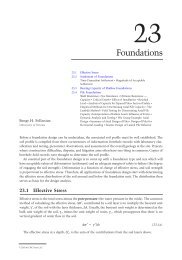
47-16 The Civil Engineering Handbook, Second EditionCQQC′A 1 A′ ANO′ 1 N1 O 1 OP′ 1 P 1 PB′ B 1 BQQDyEANOB(a)(b)FIGURE 47.13 Bending of curved beams.The deflection of a tangent at the center from a tangent at the right end, d 3 , is determined as ql 4 /128EI.The difference between d 2 and d 3 gives the centerline deflection as (5/384) x (ql 4 /EI).Curved BeamsThe beam formulas derived in the previous section are based on the assumption that the member to whichbending moment is applied is initially straight. Many members, however, are curved before a bendingmoment is applied to them. Such members are called curved beams. In the following discussion all theconditions applicable to straight-beam formulas are assumed valid, except that the beam is initially curved.Let the curved beam DOE shown in Fig. 47.13 be subjected to the load Q. The surface in which thefibers do not change in length is called the neutral surface. The total deformations of the fibers betweentwo normal sections, such as AB and A 1 B 1 , are assumed to vary proportionally with the distances of thefibers from the neutral surface. The top fibers are compressed, while those at the bottom are stretched,i.e., the plane section before bending remains plane after bending.In Fig. 47.13 the two lines AB and A 1 B 1 are two normal sections of the beam before the loads areapplied. The change in the length of any fiber between these two normal sections after bending isrepresented by the distance along the fiber between the lines A 1 B 1 and A¢B¢; the neutral surface isrepresented by NN 1 , and the stretch of fiber PP 1 is P 1 P ¢ 1 , etc. For convenience, it will be assumed thatline AB is a line of symmetry and does not change direction.The total deformations of the fibers in the curved beam are proportional to the distances of the fibersfrom the neutral surface. However, the strains of the fibers are not proportional to these distances becausethe fibers are not of equal length. Within the elastic limit the stress on any fiber in the beam is proportionalto the strain of the fiber, and hence the elastic stresses in the fibers of a curved beam are not proportionalto the distances of the fibers from the neutral surface. The resisting moment in a curved beam, therefore,is not given by the expression sI/c. Hence the neutral axis in a curved beam does not pass through thecentroid of the section. The distribution of stress over the section and the relative position of the neutralaxis are shown in Fig. 47.13b; if the beam were straight, the stress would be zero at the centroidal axisand would vary proportionally with the distance from the centroidal axis, as indicated by the dot–dashline in the figure. The stress on a normal section such as AB is called the circumferential stress.Sign ConventionsThe bending moment M is positive when it decreases the radius of curvature and negative when itincreases the radius of curvature; y is positive when measured toward the convex side of the beam andnegative when measured toward the concave side, that is, toward the center of curvature. With these signconventions, s is positive when it is a tensile stress.Circumferential StressesFigure 47.14 shows a free-body diagram of the portion of the body on one side of the section; theequations of equilibrium are applied to the forces acting on this portion. The equations obtained are© 2003 by CRC Press LLC

Theory and Analysis of Structures 47-17+Mσ dayZσ daOydaXYYFIGURE 47.14 Free-body diagram of curved beam segment.CdθRdθ + ∆dθC′RdayρA 1O′ 1∆dθP′ 1H P 1B′B 1ANeutralsurfaceO 1OO 1 = dsBAOPρyFIGURE 47.15 Curvature in a curved beam.ÚSF = z0 or sda= 0SM = z0 or M = ysdaÚ(47.17)(47.18)Figure 47.15 represents the part ABB 1 A 1 of Fig. 47.13a enlarged; the angle between the two sectionsAB and A 1 B 1 is dq. The bending moment causes the plane A 1 B 1 to rotate through an angle Ddq, therebychanging the angle this plane makes with the plane BAC from dq to (dq + Ddq); the center of curvatureis changed from C to C¢, and the distance of the centroidal axis from the center of curvature is changedfrom R to r. It should be noted that y, R, and r at any section are measured from the centroidal axis andnot from the neutral axis.It can be shown that the bending stress s is given by the relationM Ê 1s= Á1+aR Ë Zy ˆ˜R + y ¯(47.19)© 2003 by CRC Press LLC

47-18 The Civil Engineering Handbook, Second Editionin whichs is the tensile or compressive (circumferential) stress at a point at distance y from the centroidal axisof a transverse section at which the bending moment is M; R is the distance from the centroidal axis ofthe section to the center of curvature of the central axis of the unstressed beam; a is the area of the crosssection;and Z is a property of the cross-section, the values of which can be obtained from the expressionsfor various areas given in Fig. 47.17. Detailed information can be obtained from Seely and Smith (1952).Example 47.2The bent bar shown in Fig. 47.16 is subjected to a load P = 1780 N. Calculate the circumferential stressat A and B, assuming that the elastic strength of the material is not exceeded.We know from Eq. (47.19)in which a = the area of rectangular section (40 ¥ 12 = 480 mm 2 )R = 40 mmy A = –20y B = +20P = 1780 NM = –1780 ¥ 120 = –213,600 N mm.From Table 47.2.1, for rectangular section1Z =- ya Ú da R+ yP M ʈs= + Á +a aR˜Ë1 1 yZ R+y ¯Z 1 R È R+c˘=- + logeh ÍÎ R-c˙˚h = 40 mmHence,c = 20 mm40 È 40 + 20˘Z =- 1+loge0.098640 ÍÎ 40 - 20˙ ˚=PPA40 mmB40 mm120 mm12 mmSection A − BFIGURE 47.16 Bent bar.© 2003 by CRC Press LLC

Theory and Analysis of Structures 47-19hZ = 1 − c 1 c 4 5 c 6 7 c 8K − O2+ −8 K−4 R R O + 6 4 K −R O + 12 8 K −R O + ...cRR 2 RZ = −1 + 2 R 2K −c O − 2K−c O K − O − 1 chZ = 1 c 2 1 c 4 1 c 6−K−3 R O + −5 K−R O + −7 K−R O + ...cRZ = −1 + 2 hRZ = −1 + R R + c− Blog e Kh R − c OFhb 1c 1 c 2bRZ = −1 + a h ;[b 1 h + (R + c 1 )(b − b 1 )] log R +e K R −c1O − (b − bc1 )h?2R2RZ = −1 + (b + b 1 )h ;Bb 1 + b − b 1 +(R + ch1 )F log e KRR −c1O − (b − bc1 )?2hc 1c 2R2 B (R + c 1 ) log R +e K R −c1c2O − hFhZ = 1 − c 1K − O2 c 4 5 c 6+ −8 K − O + 4 R R 6 4 K −R O +7 c 8128 K −R O + ...c RZ = −1 + 2 KR −c O2− 2 K R − cO K R − cO2− 1FIGURE 47.17 Analytical expressions for Z.Therefore47.3 Trusses1780s A= + - 213600 ÊÁ +480 480 ¥ 40 Ë1 10.09861780s B= + - 213600 ÊÁ +480 480 ¥ 40 Ë1 10.0986-20ˆ˜40 - 20 ¯20 ˆ˜40 + 20 ¯= 105.4 N/mm 2 (tensile)= –45 N/mm 2 (compressive)A structure that is composed of a number of members pin-connected at their ends to form a stableframework is called a truss. If all the members lie in a plane, it is a planar truss. It is generally assumedthat loads and reactions are applied to the truss only at the joints. The centroidal axis of each memberis straight, coincides with the line connecting the joint centers at each end of the member, and lies in aplane that also contains the lines of action of all the loads and reactions. Many truss structures are threedimensionalin nature. However, in many cases, such as bridge structures and simple roof systems, thethree-dimensional framework can be subdivided into planar components for analysis as planar trusses© 2003 by CRC Press LLC

47-20 The Civil Engineering Handbook, Second Editionhc 12RZ = −1 +c 22− c 2 1R 2 − c 12 − R 2 − c 22c 2Rbhb 11RZ = − 1 + ;bc bc2 − b 1 c 212Kc22 R − 2Kc2OORO2− 1c2Kc 2c 2RR R− b 1 c 1 2K O2− 2Kc 1 c1ORO2− 1 ?c1Kc 1c 1c 4c 3b t 1RbZ = − 1 + R − a[b 1 log e (R + c 1 ) + (t − b 1 )log e (R + c 4 )+ (b − t)log e (R − c 3 ) − b log e (R − c 2 )]tbc 1c 2 c 2Rt/2t/2 bc 1 c 1c 2 c 2Rt/2The value of Z for each of these three sections may befound from the expression above by makingb 1 = b, c 2 = c 1 , and c 3 = c 4Z = − 1 + R − aRb log e KR+ c 2+ (t − b)log R + c1e K O− cR − c2O1t/2bArea = a = 2[(t − b) c 1 + bc 2 ]c 1c 1 c 1c 2 c 2Rtbc 1c 3c 2RIn the expression for the unequal I given above makec 4 = c 1 and b 1 = t, thent/2t/2c 3 c 1c 2bZ = − 1 + R − a[t log e (R + c 1 ) + (b − t) log e (R − c 3 ) − b log e (R − c 2 )]Area = a = tc 1 − (b − t)c 3 + bc 2RFIGURE 47.17 (continued).without seriously compromising the accuracy of the results. Figure 47.18 shows some typical idealizedplanar truss structures.There exists a relation between the number of members, m, the number of joints, j, and the reactioncomponents, r. The expression is© 2003 by CRC Press LLC

Theory and Analysis of Structures 47-21Warren trussPratt trussHowe trussFink trussWarren trussPratt trussBowstring trussFIGURE 47.18 Typical planar trusses.m = 2j – r (47.20)which must be satisfied if it is to be statically determinate internally. r is the least number of reactioncomponents required for external stability. If m exceeds (2j – r), then the excess members are calledredundant members, and the truss is said to be statically indeterminate.For a statically determinate truss, member forces can be found by using the method of equilibrium.The process requires repeated use of free-body diagrams from which individual member forces aredetermined. The method of joints is a technique of truss analysis in which the member forces aredetermined by the sequential isolation of joints — the unknown member forces at one joint are solvedand become known for the subsequent joints. The other method is known as method of sections, in whichequilibrium of a part of the truss is considered.Method of JointsAn imaginary section may be completely passed around a joint in a truss. The joint has become a freebody in equilibrium under the forces applied to it. The equations SH = 0 and SV = 0 may be appliedto the joint to determine the unknown forces in members meeting there. It is evident that no more thantwo unknowns can be determined at a joint with these two equations.Example 47.3A truss shown in Fig. 47.19 is symmetrically loaded and is sufficient to solve half the truss by consideringjoints 1–5. At joint 1, there are two unknown forces. Summation of the vertical components of all forcesat joint 1 gives135 – F 12 sin45° = 0which in turn gives the force in members 1 and 2, F 12 = 190 kN (compressive). Similarly, summation ofthe horizontal components givesF 13 – F 12 cos45° = 0© 2003 by CRC Press LLC

47-22 The Civil Engineering Handbook, Second Edition2A5 61135 kN3 4790 kN 90 kN90 kNA6 m 6 m 6 m 6 m135 kN6 m1F 1245°135 kN F 13245°F 12F 23F 25FIGURE 47.19 Example of the method of joints, planar truss.Substituting for F 12 gives the force in member 1–3 asF 13 = 135 kN (tensile)Now, joint 2 is cut completely, and it is found that there are two unknown forces F 25 and F 23 . Summationof the vertical components givesThereforeSummation of the horizontal components givesand henceF 23 FF 453545°F 13 3 F 34F 34 4 F 6790 kN90 kNF 12 cos45° – F 23 = 0F 23 = 135 kN (tensile)F 12 sin45° – F 25 = 0F 25 = 135 kN (compressive)After solving for joints 1 and 2, one proceeds to take a section around joint 3 at which there are nowtwo unknown forces viz. F 34 and F 35 . Summation of the vertical components at joint 3 givesF 23 – F 35 sin45° – 90 = 0Substituting for F 23 , one obtains F 35 = 63.6 kN (compressive). Summing the horizontal components andsubstituting for F 13 one gets© 2003 by CRC Press LLC

Theory and Analysis of Structures 47-23Therefore,–135 – 45 + F 34 = 0F 34 = 180 kN (tensile)The next joint involving two unknowns is joint 4. When we consider a section around it, the summationof the vertical components at joint 4 givesF 45 = 90 kN (tensile)Now, the forces in all the members on the left half of the truss are known, and by symmetry the forcesin the remaining members can be determined. The forces in all the members of a truss can also bedetermined by using the method of sections.Method of SectionsIn this method, an imaginary cutting line called section is drawnthrough a stable and determinate truss. Thus, a section divides thetruss into two separate parts. Since the entire truss is in equilibrium,any part of it must also be in equilibrium. Either of the two parts ofthe truss can be considered, and the three equations of equilibriumSF x = 0, SF y = 0, and SM = 0 can be applied to solve for memberforces.Example 47.3 above (Fig. 47.20) is once again considered. To calculatethe force in members 3–5, F 35 , section AA should be run tocut members 3–5 as shown in the figure. It is required only to considerthe equilibrium of one of the two parts of the truss. In this case,the portion of the truss on the left of the section is considered. Theleft portion of the truss as shown in Fig. 47.20 is in equilibrium underthe action of the forces viz. the external and internal forces. Consideringthe equilibrium of forces in the vertical direction, one canobtain135 kNF 3545°90 kNFIGURE 47.20 Example of themethod of sections, planar truss.AA135 – 90 + F 35 sin45˚ = 0Therefore, F 35 is obtained asThe negative sign indicates that the member force is compressive. The other member forces cut by thesection can be obtained by considering the other equilibrium equations viz. SM = 0. More sections canbe taken in the same way to solve for other member forces in the truss. The most important advantageof this method is that one can obtain the required member force without solving for the other memberforces.Compound TrussesF =-45 235kNA compound truss is formed by interconnecting two or more simple trusses. Examples of compoundtrusses are shown in Fig. 47.21. A typical compound roof truss is shown in Fig. 47.21a in which twosimple trusses are interconnected by means of a single member and a common joint. The compoundtruss shown in Fig. 47.21b is commonly used in bridge construction, and in this case, three membersare used to interconnect two simple trusses at a common joint. There are three simple trusses interconnectedat their common joints, as shown in Fig. 47.21c.© 2003 by CRC Press LLC

47-24 The Civil Engineering Handbook, Second Edition(a) Compound roof truss(b) Compound bridge trussFIGURE 47.21 Compound truss.The method of sections may be used to determine the member forces in the interconnecting membersof compound trusses, similar to those shown in Fig. 47.21a and b. However, in the case of a cantileveredtruss the middle simple truss is isolated as a free-body diagram to find its reactions. These reactions arereversed and applied to the interconnecting joints of the other two simple trusses. After the interconnectingforces between the simple trusses are found, the simple trusses are analyzed by the method ofjoints or the method of sections.47.4 FramesFrames are statically indeterminate in general; special methods are required for their analysis. Slopedeflection and moment distribution methods are two such methods commonly employed. Slope deflectionis a method that takes into account the flexural displacements such as rotations and deflections andinvolves solutions of simultaneous equations. Moment distribution, on the other hand, involves successivecycles of computation, each cycle drawing closer to the “exact” answers. The method is more laborintensive but yields accuracy equivalent to that obtained from the “exact” methods.Slope Deflection Method(c) Cantilevered constructionThis method is a special case of the stiffness method of analysis. It is a convenient method for performinghand analysis of small structures.Let us consider a prismatic frame member AB with undeformed position along the x axis deformed intoconfiguration p, as shown in Fig. 47.22. Moments at the ends of frame members are expressed in terms ofthe rotations and deflections of the joints. It is assumed that the joints in a structure may rotate or deflect,but the angles between the members meeting at a joint remain unchanged. The positive axes, along withthe positive member-end force components and displacement components, are shown in the figure.yV ABM AB Ay APθ Aψ ABV BA M BAψ ABθ BBy B∆ ABxabFIGURE 47.22 Deformed configuration of a beam.© 2003 by CRC Press LLC

Theory and Analysis of Structures 47-25The equations for end moments may be written asMM2EI= 2q + q -3yl( ) +2EI= 2q + q -3ylMAB A B AB FAB( ) +MBA B A AB FBA(47.21)in which M FAB and M FBA are fixed-end moments at supports A and B, respectively, due to the appliedload. y AB is the rotation as a result of the relative displacement between member ends A and B given asD y + y= =1 1y ABAB A B(47.22)where D AB is the relative deflection of the beam ends. y A and y B are the vertical displacements at ends Aand B. Fixed-end moments for some loading cases may be obtained from Fig. 47.8. The slope deflectionequations in Eq. (47.21) show that the moment at the end of a member is dependent on memberproperties EI, length l, and displacement quantities. The fixed-end moments reflect the transverse loadingon the member.Frame Analysis Using Slope Deflection MethodThe slope deflection equations may be applied to statically indeterminate frames with or without sidesway. A frame may be subjected to side sway if the loads, member properties, and dimensions of theframe are not symmetrical about the centerline. Application of the slope deflection method can beillustrated with the following example.Example 47.4Consider the frame shown in Fig. 47.23 subjected to side sway D to the right of the frame. Equation (47.21)can be applied to each of the members of the frame as follows:Member AB:M2EI Ê 3Dˆ= Á2q+ q - ˜ + M6 Ë 20 ¯AB A B FABq A = 0,MM2EIÊ= + - MËÁˆ˜ +20 2 3Dq q20 ¯BA B A FBAFAB= M = 0FBAB180 kN3 m 6 mC6 mAEI − Same forall members9 mDFIGURE 47.23 Example of the slope deflection method.© 2003 by CRC Press LLC

47-26 The Civil Engineering Handbook, Second EditionHenceMM BAAB2EI= qB-3y6( )2EI= -( y )20 2q3 B(47.23)(47.24)in whichy = D 6Member BC:MM2EI= ( 2q+ q - 3 ¥ 0)+M9BC B C FBCCB= 2EI 2 q + q - 3 ¥ 0C B9( ) +MFCB2180 ¥ 3 ¥ 6M FBC =-=-240ft-kips29M2180¥ 3 ¥ 6=-= 120 ft-kips9FCB 2HenceM2EI= ( 2q+ q )- 2409BC B C(47.25)2EI ( 2 ) + 899M CB= q C+ q B(47.26)Member CD:M2EIÊ 3Dˆ= Á2q+ q - ˜ + M9 Ë 30 ¯CD C D FCDq D = 0,MM2EIÊ 3Dˆ= Á2q+ q - ˜ + M9 Ë 30 ¯DC D C FDCFCD= M = 0FDCHenceMCDM2EI Ê 1 ˆ 2EI= Á2qC- ¥ 6y˜ = 2qC-2y9 Ë 3 ¯ 9DC( )2EI Ê 1 ˆ 2EI= Á qC- ¥ 6y˜ = qC-2y9 Ë 3 ¯ 9( )(47.27)(47.28)© 2003 by CRC Press LLC

Theory and Analysis of Structures 47-27Considering moment equilibrium at joint BSubstituting for M BA and M BC , one obtainsSM B = M BA + M BC = 0EI 10 qB+ 2 qC- 9 y9or( ) =2402160110 qB+ 2qC- 9y= EI(47.29)Considering moment equilibrium at joint CSubstituting for M CB and M CD we getSM C = M CB + M CD = 02EI 4 qC+ qB- 2 y9or( ) =-120qB4qC2y+ - = - 540EI(47.30)For summation of base shears equal to zero, we haveorSH = H A + H D = 0M + M M + M+6 9AB BA CD DCSubstituting for M AB , M BA , M CD , and M DC and simplifying= 02qB+ 12qC- 70y= 0(47.31)Solution of Eqs. (47.29) to (47.31) results in342.7qB=EI.q = - 169 1CEI© 2003 by CRC Press LLC

47-28 The Civil Engineering Handbook, Second Editionandy = 103.2EI(47.32)Substituting for q B , q C , and y from Eq. (47.32) into Eqs. (47.23) to (47.28) we getMoment Distribution MethodM AB = 11.03 kNmM BA = 125.3 kNmM BC = –125.3 kNmM CB = 121 kNmM CD = –121 kNmM DC = –83 kNmThe moment distribution method involves successive cycles of computation, each cycle drawing closerto the “exact” answers. The calculations may be stopped after two or three cycles, giving a very goodapproximate analysis, or they may be carried out to whatever degree of accuracy is desired. Momentdistribution remains the most important hand-calculation method for the analysis of continuous beamsand frames, and it may be solely used for the analysis of small structures. Unlike the slope deflectionmethod, this method does require the solution to simultaneous equations.The terms constantly used in moment distribution are fixed-end moments, the unbalanced moment,distributed moments, and carryover moments. When all of the joints of a structure are clamped to preventany joint rotation, the external loads produce certain moments at the ends of the members to which theyare applied. These moments are referred to as fixed-end moments. Initially the joints in a structure areconsidered to be clamped. When the joint is released, it rotates if the sum of the fixed-end moments atthe joint is not zero. The difference between zero and the actual sum of the end moments is the unbalancedmoment. The unbalanced moment causes the joint to rotate. The rotation twists the ends of the membersat the joint and changes their moments. In other words, rotation of the joint is resisted by the members,and resisting moments are built up in the members as they are twisted. Rotation continues until equilibriumis reached — when the resisting moments equal the unbalanced moment — at which time thesum of the moments at the joint is equal to zero. The moments developed in the members resistingrotation are the distributed moments. The distributed moments in the ends of the member cause momentsin the other ends, which are assumed fixed; these are the carryover moments.Sign ConventionThe moments at the end of a member are assumed to be positive when they tend to rotate the memberclockwise about the joint. This implies that the resisting moment of the joint would be counterclockwise.Accordingly, under a gravity loading condition the fixed-end moment at the left end is assumed ascounterclockwise (–ve) and at the right end as clockwise (+ve).Fixed-End MomentsFixed-end moments for several cases of loading may be found in Fig. 47.8. Application of momentdistribution may be explained with reference to a continuous beam example, as shown in Fig. 47.24.Fixed-end moments are computed for each of the three spans. At joint B the unbalanced moment isobtained and the clamp is removed. The joint rotates, thus distributing the unbalanced moment to theB ends of spans BA and BC in proportion to their distribution factors. The values of these distributedmoments are carried over at one half rate to the other ends of the members. When equilibrium is reached,© 2003 by CRC Press LLC

Theory and Analysis of Structures 47-29902 (Uniformly distributed)A3EI B EI C EI39 7.5D−500.6 0.4 0.45 0.5550 −150 150 −1041043060 40 −20.7 −25.3−10.4 20 −12.7+6.2 +4.2 −9.0 −11.03.1 −4.5 2.1 −5.5+2.7 +1.8−0.9 −1.21.4−0.50.9−0.6+0.3 +0.2−0.4 −0.5−15.5 119.2 −119.2 +142 −142 85.2FIGURE 47.24 Example of a continuous beam by moment distribution.joint B is clamped in its new rotated position and joint C is released afterwards. Joint C rotates underits unbalanced moment until it reaches equilibrium, the rotation causing distributed moments in theC ends of members CB and CD and their resulting carryover moments. Joint C is now clamped and joint Bis released. This procedure is repeated again and again for joints B and C, the amount of unbalancedmoment quickly diminishing, until the release of a joint causes negligible rotation. This process is calledmoment distribution.The stiffness factors and distribution factors are computed as follows:The fixed-end moments areDFDFDFDFBABCCBCDI=KBA20= = 0.6Â K I 20 + I 30I=KBC30= = 0.4Â K I 20 + I 30I=KCB30= = 0.45Â K I 30 + I 25I=KCD25= = 0.55Â K I I 30 + I 25MFAB =- 50; MFBC =- 150;MFCD=-104M = 50; M = 150;M = 104FBA FCB FDCWhen a clockwise couple is applied near the end of a beam, a clockwise couple of half the magnitudeis set up at the far end of the beam. The ratio of the moments at the far and near ends is defined as thecarryover factor, 0.5 in the case of a straight prismatic member. The carryover factor was developed forcarrying over to fixed ends, but it is applicable to simply supported ends, which must have final momentsof zero. It can be shown that the beam simply supported at the far end is only three fourths as stiff asthe one that is fixed. If the stiffness factors for end spans that are simply supported are modified by threefourths, the simple end is initially balanced to zero and no carryovers are made to the end afterward.This simplifies the moment distribution process significantly.© 2003 by CRC Press LLC

47-30 The Civil Engineering Handbook, Second Edition3A EI BC EIEI10D1020202EI 2EI20E20F20+15.82+0.20+3.12+12.5 0.2581.64+ 0.39+ 6.25+25.0+50.0 0.50+80.86−0.39+1.57−1.57+6.25−25.00.25 +100.0 0.25 0.25−100.0+ 12.5− 25.0− 1.56− 12.5− 0.39+ 3.13− 26.95− 0.79+ 0.20− 97.46−50.0+12.5+ 3.13+ 0.20−34.17−53.92− 0.79− 3.130.50−50.0− 25.0− 1.57− 0.40− 26.97FIGURE 47.25 Example of a nonsway frame by moment distribution.Moment Distribution for FramesMoment distribution for frames without side sway is similar to that for continuous beams. The exampleshown in Fig. 47.25 illustrates the applications of moment distribution for a frame without side sway.Similarly,EIDF = 20BAEI EI+ +20 20DFMMBEFBCFBE2EI20= 0.25= 05 .; DFBC= 025 .= 0100;MFCB= 100= 50;M = -50FEBStructural frames are usually subjected to side sway in one direction or the other, due to asymmetryof the structure and eccentricity of loading. The sway deflections affect the moments, resulting in anunbalanced moment. These moments could be obtained for the deflections computed and added to theoriginally distributed fixed-end moments. The sway moments are distributed to columns. Should a framehave columns all of the same length and the same stiffness, the side sway moments will be the same foreach column. However, should the columns have differing lengths or stiffnesses, this will not be the case.The side sway moments should vary from column to column in proportion to their I/l 2 values.The frame in Fig. 47.26 shows a frame subjected to sway. The process of obtaining the final momentsis illustrated for this frame.The frame sways to the right, and the side sway moment can be assumed in the ratio40020 : 3002 220(or) 1 : 0.75© 2003 by CRC Press LLC

Theory and Analysis of Structures 47-31B1.5 (Uniformly distributed)C1060020 4003002010AD30+109.7+ 0.3+ 2.90.43+31.5+25+500.57− 112.5− 36+ 42− 6.7+ 3.8− 0.6+ 0.3− 109.748.8− 1.2+ 1.9− 13.4+21− 72+ 112.5−48.8− 0.70.64 13.06− 7.6−40.50.36−50+50010.005.504.502.44FIGURE 47.26 Example of a sway frame by moment distribution.Final moments are obtained by adding distributed fixed-end moments and 13.06/2.99 times thedistributed assumed side sway moments.Method of Consistent DeformationsThis method makes use of the principle of deformation compatibility to analyze indeterminate structures.It employs equations that relate the forces acting on the structure to the deformations of the structure.These relations are formed so that the deformations are expressed in terms of the forces, and the forcesbecome the unknowns in the analysis.Let us consider the beam shown in Fig. 47.27a. The first step, in this method, is to determine thedegree of indeterminacy or the number of redundants that the structure possesses. As shown in the figure,the beam has three unknown reactions, R A , R C , and M A . Since there are only two equations of equilibriumavailable for calculating the reactions, the beam is said to be indeterminate to the first degree. Restraintsthat can be removed without impairing the load-supporting capacity of the structure are referred to asredundants.Once the number of redundants are known, the next step is to decide which reaction is to be removedin order to form a determinate structure. Any one of the reactions may be chosen to be the redundant,provided that a stable structure remains after the removal of that reaction. For example, let us take thereaction R C as the redundant. The determinate structure obtained by removing this restraint is thecantilever beam shown in Fig. 47.27b. We denote the deflection at end C of this beam, due to P, by D CP .The first subscript indicates that the deflection is measured at C, and the second subscript indicates that© 2003 by CRC Press LLC

47-32 The Civil Engineering Handbook, Second Edition− 31.700.57+28.5+ 7.4− 4.2+31.70.4328.30+ 1.3− 2.1+14.80+14.300.64−100+1000−75.0+75.00− 3.2+ 21.5+ 50−100−28.3+ 0.8+ 8.4+37.5−75.00.361.59Total2.991.40172.4+123.6+ 48.820− 28.8−138.5+109.7−109.7+138.5+ 28.8−172.4−123.6− 48.810.001.44 8.6211.44FIGURE 47.26 (continued).M AR AAPBL/2 L/2(a) Actual structureCR C∆ CRR C(c) Determinate structuresubject to redundantPb) Determinate structuresubject to actual loads∆ CPP316 PL 1116 P 516 P(d)FIGURE 47.27 Beam with one redundant reaction.the deflection is due to the applied load P. Using the moment area method, it can be shown that D CP =5PL 3 /48EI. The redundant R C is then applied to the determinate cantilever beam, as shown in Fig. 47.27c.This gives rise to a deflection D CR at point C, the magnitude of which can be shown to be R C L 3 /3EI.© 2003 by CRC Press LLC

Theory and Analysis of Structures 47-33In the actual indeterminate structure, which is subjected to the combined effects of the load P andthe redundant R C , the deflection at C is zero. Hence the algebraic sum of the deflection D CP in Fig. 47.27band the deflection D CR in Fig. 47.27c must vanish. Assuming downward deflections to be positive, we writeorfrom whichDCP- D =0CR3 35PLRLC- = 048EI3EIR C= 516 P(47.33)Equation (47.33), which is used to solve for the redundant, is referred to as an equation of consistentdeformations.Once the redundant R C has been evaluated, the remaining reactions can be determined by applyingthe equations of equilibrium to the structure in Fig. 47.27a. Thus SF y = 0 leads toand SM A = 0 givesR A= P- 5 =16 P 1116 PPL 5M A= - =2 16 PL 316 PLA free body of the beam, showing all the forces acting on it, is shown in Fig. 47.27d.The steps involved in the method of consistent deformations follow:1. The number of redundants in the structure are determined.2. Enough redundants to form a determinate structure are removed.3. The displacements that the applied loads cause in the determinate structure at the points wherethe redundants have been removed are calculated.4. The displacements at these points in the determinate structure, due to the redundants, areobtained.5. At each point where a redundant has been removed, the sum of the displacements calculated insteps 3 and 4 must be equal to the displacement that exists at that point in the actual indeterminatestructure. The redundants are evaluated using these relationships.6. Once the redundants are known, the remaining reactions are determined using the equations ofequilibrium.Structures with Several RedundantsThe method of consistent deformations can be applied to structures with two or more redundants. Forexample, the beam in Fig. 47.28a is indeterminate to the second degree and has two redundant reactions.If the reactions at B and C are selected to be the redundants, then the determinate structure obtainedby removing these supports is the cantilever beam, shown in Fig. 47.28b. To this determinate structurewe apply separately the given load (Fig. 47.28c) and the redundants R B and R C , one at a time (Fig. 47.28dand e).Since the deflections at B and C in the original beam are zero, the algebraic sum of the deflections inFig. 47.28c, d, and e at these same points must also vanish. Thus© 2003 by CRC Press LLC

47-34 The Civil Engineering Handbook, Second EditionW 1 W 2M ABA L/2 L/2CR AR B(a)R CAB(b)CW 1 W 2∆ BP(c)∆ CP∆ BB∆ CBR B(d)∆ CC∆ BC(e)R CFIGURE 47.28 Beam with two redundant reactions.D - D - D = 0BP BB BCD - D - D = 0CP CB CC(47.34)It is useful in the case of complex structures to write the equations of consistent deformations in theformDD- d R - d R = 0BP BB B BC C- d R - d R = 0CP CB B CC C(47.35)in which d BC , for example, denotes the deflection at B due to a unit load at C in the direction of R C .Solution of Eq. (47.35) gives the redundant reactions R B and R C .Example 47.5Determine the reactions for the beam shown in Fig. 47.29, and draw its shear force and bending momentdiagrams.It can be seen from the figure that there are three reactions viz. M A , R A , and R C , one more than thatrequired for a stable structure. The reaction R C can be removed to make the structure determinate. Weknow that the deflection at support C of the beam is zero. One can determine the deflection d CP at Cdue to the applied load on the cantilever in Fig. 47.29b. In the same way the deflection d CR at C due tothe redundant reaction on the cantilever (Fig. 47.29c) can be determined. The compatibility equationgives© 2003 by CRC Press LLC

Theory and Analysis of Structures 47-35M A20 kN 10 kNADCEIEIR A 2 m 2 m 2 mB(a)R C20 kN 10 kNδ CP40EI100EI(b)20EIδ CRR C4R CEI(c)6.25 kN+ +−13.75 kN10 kN−5 kNm(d)7.5 kNm+−20 kNmFIGURE 47.29 Example 47.5.dCP- d =0CRBy moment area method,ddCP20ʈ= ¥ 2 ¥ 1+ 1 20 2 40¥ ¥ 2 ¥ ¥ 2 + ¥ 2 ¥ 3 + 1 60 2 1520¥ ¥ 2 ¥ Á ¥ 2 + 2˜ =EI 2 EI 3 EI 2 EI Ë 3¯ 3EI124REICCR= ¥ ¥ ¥ ¥ =423464R3EISubstituting for d CP and d CR in the compatibility equation, one obtains,C15203EI64R- C=03EI© 2003 by CRC Press LLC

47-36 The Civil Engineering Handbook, Second Editionfrom whichBy using statical equilibrium equations we getR C = 23.75 kN≠R A = 6.25 kN≠and M A = 5 kNm.The shear force and bending moment diagrams are shown in Fig. 47.29d.1. Solutions to fix-based portal frames subjected to various loading: Fig. 47.30 shows the bendingmoment diagram and reaction forces of fix-based portal frames subjected to loading typicallyencountered in practice. Closed-form solutions are provided for moments and end forces tofacilitate a quick solution to the simple frame problem.2. Solutions to pin-based portal frames subjected to various loading: Fig. 47.31 shows the bendingmoment diagram and reaction forces of pin-based portal frames subjected to loading typicallyencountered in practice. Closed-form solutions are provided for moments and end forces tofacilitate a quick solution to the simple frame problem.Frame II bB C Coefficients:I c I c a = (ILb /L)/(I c /h)A Db 1 = a + 2 b 2 = 6a + 1FRAME DATAhw per unit length−− B +B C−2LA DA +H AM AV A−C −wL 28+ DV DH DM DM A = M D = 1w2Lb21M B = M C = −6 w bL 2= - 2M A1M max =wL 28+ M BV A = V D = wL2H A = H D = 3M AhFIGURE 47.30 Rigid frames with fixed supports.© 2003 by CRC Press LLC

Theory and Analysis of Structures 47-37aABhCw per unitheightDM A =wh 2 a + 3 4a + 14 6b 1 b 2wh 28−B+AV DV AH AM AM B = wh24h/2−C −a- +2a6b 1 b 2+ D H LM DV DM D = wh2 a + 3 4a + 1+M - -4 6b 1 b C = wh2 a 2a24 6b 1 b 2wh(2a + 3)H D = H A = -(wh - H D8b ) V A = - V D = - wh2 a1 Lb 2Constants:3Paa 1 aa 1 =a X 1 =hb 2−B CPPB +C −ALD− A H A + DM AV DM DH DM A = − Pa + X 1M B = X 1M D = +Pa − X 1 M C = − X 1V A = −V D = − 2X 1LH A = −H D = − PFIGURE 47.30 (continued).47.5 PlatesBending of Thin PlatesA plate in which its thickness is small compared to the other dimensions is called a thin plate. The planeparallel to the faces of the plate and bisecting the thickness of the plate, in the undeformed state, is calledthe middle plane of the plate. When the deflection of the middle plane is small compared with thethickness, h, it can be assumed that1. There is no deformation in the middle plane.2. The normals of the middle plane before bending are deformed into the normals of the middleplane after bending.3. The normal stresses in the direction transverse to the plate can be neglected.© 2003 by CRC Press LLC

47-38 The Civil Engineering Handbook, Second EditionPBCB +−C −L/2AD−AH AM A+DH DM DV AV DM3a + 1A = − Ph2 b 2M3aB = + Ph2 b 2M 3a + 1D = + Ph M3a2 b C = − Ph22 b 2H A = −H D = − P2V A = −V D = −2M BLBAaPbCDH AM A−−BA +V APabL−C −+V DDH DM DM A = Pab 1 −b − aL 2b 1 2Lb 2M B = − Pab 1 b - a +L b 1 2Lb 2+M D = Pab 1 b − aM C = − Pab 1 -b − aL b 1 2Lb 2L 2b 1 2Lb 2V A = Pb a(b − a)1 + V D = P − VLAL 2 b 23PabH A = H D =2Lhb 1FIGURE 47.30 (continued).Based on these assumptions, all stress components can be expressed by deflection w of the plate. w isa function of the two coordinates (x, y) in the plane of the plate. This function has to satisfy a linearpartial differential equation, which, together with the boundary conditions, completely defines w.Figure 47.32a shows a plate element cut from a plate whose middle plane coincides with the xy plane.The middle plane of the plate subjected to a lateral load of intensity, q, is shown in Fig. 47.32b. It canbe shown, by considering the equilibrium of the plate element, that the stress resultants are given asÊ2M X=-∂+ ∂ 2w w ˆDÁn22Ë ∂˜x ∂ y ¯Ê2=-∂Á + ∂ 2w w ˆMyDn22Ë ∂ ∂˜y x ¯(47.36)© 2003 by CRC Press LLC

Theory and Analysis of Structures 47-39BCI 1 I 1hI 2LADCoefficients:α = (I b /L)/(I c /h)β = 2α + 3FRAME DATAw per unit lengthB C− −B +L/2−C −wL 28ADH AV AADV DH DM B = M C = − wL 24bV A = V D = wL2M max =wL 28H A = H D = − M Bh+ M BFIGURE 47.31 Rigid frames with pinned supports.=- = -nMxyMyxD1( ) ∂2w∂x∂yV y= ∂ 3w+ 23- n∂ y( )V x= ∂ 3w+ 2 - n3∂ x( )3∂ w∂y∂x3∂ w∂x∂yQ =- ∂ Ê2yD∂+ ∂ 2w w ˆ∂Á 2 2y Ë ∂˜x ∂ y ¯22(47.37)(47.38)(47.39)where( ) ∂R = 2D 1-n2w∂x∂yM x and M y = the bending moments per unit length in the x and y directions, respectivelyM xy and M yx = the twisting moments per unit lengthQ x and Q y = the shearing forces per unit length in the x and y directions, respectivelyV x and V y =are the supplementary shear forces in the x and y directions, respectivelyR = the corner forceD = Eh 3 /12(1 – n 2 ), the flexural rigidity of the plate per unit lengthE = the modulus of elasticity; and n is Poisson’s ratio(47.40)© 2003 by CRC Press LLC

47-40 The Civil Engineering Handbook, Second Edition−B +BCwh 2 C −w per unit8height+LA H A D H DADV A V DH D = − MMh CB = w h 2 −4 2 = > + 1M H A = −(wh − C = w h 2 − H D )4 2 = > − 1hh/2V A = −V D = − 2 w Lh 2PBCPB +Pa−C−PahAaLDH AAD H DV AV DM B = −M c = PaH A = H d = PV A = −V D = − 2P aLMoment at Loads = ±PaFIGURE 47.31 (continued).The governing equation for the plate is obtained as44∂ w w+ 2∂4∂ x ∂x∂y2 24w+ ∂ =4∂ yqD(47.41)Any plate problem should satisfy the governing Eq. (47.41) and boundary conditions of the plate.Boundary ConditionsThere are three basic boundary conditions for plates. These are the clamped edge, simply supported edge,and free edge.Clamped EdgeFor this boundary condition, the edge is restrained such that the deflection and slope are zero along theedge. If we consider the edge x = a to be clamped, we have© 2003 by CRC Press LLC

Theory and Analysis of Structures 47-41P−BCB +C −L/2LAH AMD DADV A V DM B = −M C = + P 2 hV A = − V D = −P L h H A = −H D = −P 2a P b−−− BC −BCPabLH A ADH DLADV A V DM B = Mc = − P ab . 3L 2 >V A = P L b V D = P L a H A = H D = − Mh BhhFIGURE 47.31 (continued).Ê ∂wˆ( w) = 0;x aÁ ˜ = 0=Ë ∂x¯(47.42)Simply Supported EdgeIf the edge x = a of the plate is simply supported, the deflection w along this edge must be zero. At thesame time this edge can rotate freely with respect to the edge line. This means thatx=a2Ê ∂ w ˆ( w) = 0;x aÁ ˜ = 0=2Ë ∂x¯x=a(47.43)Free EdgeIf the edge x = a of the plate is entirely free, there are no bending and twisting moments and also verticalshearing forces. This can be written in terms of w, the deflection, asÊ2 2∂ w w+ ∂ ˆÁn20Ë ∂˜ =2x ∂ y ¯Ê ∂ wÁË ∂xx=a3 3+ ( 2 - n∂3 )w ˆ2 ˜ = 0∂x∂y¯x=a(47.44)© 2003 by CRC Press LLC

47-42 The Civil Engineering Handbook, Second Editiondd xyδMy δMx M y + dy Mδ x + dxy δ xδMyx M yx + dyδMxy δ y M xy + dxδxδQy δQx Q y + dy Q x + dxδ y δ x(a)M yM yxM xyM xδMy M y + dyδ yδMyx M yx + dyδ yδMx M x + dxδ xδMxy M xy + dxδ xQ yQ xxδQy Q y + dyδ yδQx Q x + dxδ xyz(b)FIGURE 47.32 (a) Plate element. (b) Stress resultants.baq oq o Sinxπx πySina byzFIGURE 47.33 Rectangular plate under sinusoidal loading.Bending of Rectangular PlatesThe plate bending problem may be solved by referring to the differential Eq. (47.41). The solution,however, depends on the loading and boundary conditions. Consider a simply supported plate subjectedto a sinusoidal loading, as shown in Fig. 47.33. The differential Eq. (47.41) in this case becomes4 4∂ w w+ 2∂4 2∂x∂x∂y24w q+ ∂ =4∂ yoD sinp xa sin p yb(47.45)© 2003 by CRC Press LLC

Theory and Analysis of Structures 47-43The boundary conditions for the simply supported edges arew = 0,w = 0,The deflection function becomes2∂ w= 0 for x = 0 and x = a∂x 22∂ w2= 0 for y = 0 and y = b∂ y(47.46)pw = w 0sin xa sin p yb(47.47)which satisfies all the boundary conditions in Eq. (47.46). w 0 must be chosen to satisfy Eq. (47.45).Substitution of Eq. (47.47) into Eq. (47.45) gives24 Ê 1 1 ˆp Á +2 2 w0Ë aqo˜ =b ¯ DThe deflection surface for the plate can, therefore, be found asw =qD1 sinx1 a sin yop p4 ʈbp Á +2 2˜Ë a b ¯(47.48)Using Eqs. (47.48) and (47.36), we find expression for moments asMMMxyxyqo=2 Ê 1 1 ˆp Á +2 2˜Ë a b ¯qo=2 Ê 1 1 ˆp Á +2 2˜Ë a b ¯22Ê 1 n ˆÁ +2 2˜Ë a b ¯sin p xa sin p ybÊ n 1 ˆÁ +2 2˜Ë a b ¯sin p xa sin p ybqo(1- n)px=cos22 Ê 1 1 ˆ a cos pybp Á +2 2˜abË a b ¯(47.49)Maximum deflection and maximum bending moments that occur at the center of the plate can be writtenby substituting x = a/2 and y = b/2 in Eq. (47.49) asM xwmax( ) =maxqo=4 ÊD1 1 ˆp Á +2 2˜Ë a b ¯qo2 Ê 1 1 ˆp Á +2 2˜Ë a b ¯22Ê 1 n ˆÁ +2 2˜Ë a b ¯(47.50)© 2003 by CRC Press LLC

47-44 The Civil Engineering Handbook, Second Edition( M y ) =max2 Ê 1 1 ˆp Á +2 2˜Ë a b ¯If the plate is square, then a = b and Eq. (47.50) becomesqo2Ê n 1 ˆÁ +2 2˜Ë a b ¯wmax4qoa=44pD1 + nMx My qoamaxmax p( ) = ( ) =( )4 2 2(47.51)If the simply supported rectangular plate is subjected to any kind of loading given byq= q( x,y)(47.52)the function q(x, y) should be represented in the form of a double trigonometric series as • •mpxnpyqxy ( , ) = qmnsin sina bm=1 n = 1(47.53)in which q mn is given byqmna b4q , sin m x sinab ÚÚ xy p n p ya bdxdy= ( )0 0(47.54)From Eqs. (47.45) and (47.52) to (47.54) we can obtain the expression for deflection as1w =p D• •q mn4 2m=1 n = 12ma+ n 2ʈÁ 2 2 ˜Ë b ¯sin m p x sin n p ya b(47.55)If the applied load is uniformly distributed of intensity q o , we haveand from Eq. (47.54) we obtain( ) =qxy ,q oqmnabqom x n yab a b dxdy qo= 4 ppsin sin=Ú Ú162p mn00(47.56)in which m and n are odd integers. q mn = 0 if m or n or both are even numbers. Finally, the deflectionof a simply supported plate subjected to a uniformly distributed load can be expressed asw16q o=6p D• •ÂÂm=1 n=1m pxn pysin sina bmn m a+ n 22 2ʈÁ 2 2 ˜Ë b ¯(47.57)© 2003 by CRC Press LLC

Theory and Analysis of Structures 47-45wherem = 1, 3, 5, …n = 1, 3, 5. …The maximum deflection occurs at the center. Its magnitude can be evaluated by substituting x = a/2and y = b/2 in Eq. (47.57) as(47.58)Equation (47.58) is a rapid converging series. A satisfactory approximation can be obtained by takingonly the first term of the series; for example, in the case of a square plate,Assuming n = 0.3, the maximum deflection can be calculated aswmax16qo=6p Dw max• •ÂÂm=1 n=144qoa= =6p Dw max=m + n(-1)- 122 2Êmn Ám 2 2a+ n ˆ˜Ë b ¯40.00416 q oa4o0.0454 q a3The expressions for bending and twisting moments can be obtained by substituting Eq. (47.57) intoEq. (47.36). Figure 47.34 shows some loading cases and the corresponding loading functions.If the opposite edges at x = 0 and x = a of a rectangular plate are simply supported, the solution takingthe deflection function asE hD2•m xw =  Y sin pmam=1(47.59)can be adopted. Equation (47.59) satisfies the boundary conditions w = 0 and ∂ 2 w/∂x 2 = 0 on the twosimply supported edges. Y m should be determined such that it satisfies the boundary conditions alongthe edges y = +b/–2 of the plate shown in Fig. 47.35 and also the equation of the deflection surface4 4∂ w w+ 2∂4 2∂x∂x∂y24w qo+ ∂ =4∂ y D(47.60)q o being the intensity of the uniformly distributed load.The solution for Eq. (47.60) can be taken in the formw = w 1+ w 2(47.61)for a uniformly loaded simply supported plate. w 1 can be taken in the formq o 4( )3 3w1= - 2ax + a x24D x(47.62)representing the deflection of a uniformly loaded strip parallel to the x axis. It satisfies Eq. (47.60) andalso the boundary conditions along x = 0 and x = a.The expression w 2 has to satisfy the equation44w22+ 2∂ w4 2 2∂∂x∂x∂y4+ ∂ w∂ y24= 0(47.63)© 2003 by CRC Press LLC

47-46 The Civil Engineering Handbook, Second EditionNo.Loadq(x,y) = Σ mΣ n q mn sinmπx nπysina bXExpansion Coefficientsq mn1abq o16qoq mn =π 2mn(m, n = 1, 3, 5,....)Z,wYX2abq o− 8q o cosmπq mn =π 2 mn(m, n = 1, 3, 5,....)Z,wY3d/2ηd/2Z,wξXqb oc/2c/2aY16qo mπξ nπηp mn = sin sinπ 2mna b× sin mπc nπdsin2a2b(m, n = 1, 3, 5,....)X4ηPb4qo mπξ nπηq mn = sin sinaba bZ,wξaY(m, n = 1, 3, 5,....)No.5Loadq(x,y) = Σ Σ q mn sin mπx nπysinm n a bXbExpansion Coefficientsq mn8qo q mn = for m,n = 1, 3, 5,....π 2mnq oq oZ,wYa/2a/216qo m = 2, 6, 10,....q mn = for ;π 2mnn = 1, 3, 5,....6Xξab4qq mn =πan o mπ ξ sina(m,n = 1, 2, 3, ....)Z,wYFIGURE 47.34 Typical loading on plates and loading functions.© 2003 by CRC Press LLC

Theory and Analysis of Structures 47-47ab/2b/2xFIGURE 47.35 Rectangular plate.yand must be chosen such that Eq. (47.61) satisfies all boundary conditions of the plate. Taking w 2 in theform of series given in Eq. (47.59), it can be shown that the deflection surface takes the form4 •o 4 3 3qoa24D Âm=1qw =24D x - 2ax + a x( ) + +C sinh m p y D m p y cosh m p y ˆsin m p+ xm+ m˜a a a ¯ aÊA cosh m p y B m p y sinh m pÁymmË a a a(47.64)Observing that the deflection surface of the plate is symmetrical with respect to the x axis, only evenfunctions of y are kept in Eq. (47.64); therefore, C m = D m = 0. The deflection surface takes the form4 •o 4 3 3qoa( ) + Amcosh m y +qw = - +24D x 2ax a x24DÂm=1ÊÁËp ˆB m p ym sinh m p y ˜ sin m p xa a a ¯ a(47.65)Developing the expression in Eq. (47.62) into a trigonometric series, the deflection surface in Eq. (47.65)is written as4 •q ʈoaw = Á+ +5 5 m m˜D Ë4m A cosh m p y B m p y sin m p y sin m p xpa a a ¯ am=1(47.66)Substituting Eq. (47.5.30) in the boundary conditions2∂ ww = 0,= 02∂y(47.67)one obtains the constants of integration A m and B m , and the expression for deflection may be written as4 •4q a 1 Ê+w =Â-+D m ËÁ1tanh 2cosh 2 yoamamamam55p2cosh ab 2coshm=1,3,5...mam2yˆ˜b sinh 2 amy sin m p xb ¯ a(47.68)in which a m = mpb/2a.Maximum deflection occurs at the middle of the plate, x = a/2, y = 0, and is given bywmax4 •o5D Âm=1,3,5,...4q a=pm -1-12 Ê mtanh m + 21 -aa ˆ5 Á˜m Ë 2cosh am¯( )(47.69)© 2003 by CRC Press LLC

47-48 The Civil Engineering Handbook, Second EditionThe solutions of plates with arbitrary boundary conditions are complicated. It is possible to make somesimplifying assumptions for plates with the same boundary conditions along two parallel edges in orderto obtain the desired solution. Alternately, the energy method can be applied more efficiently to solveplates with complex boundary conditions. However, it should be noted that the accuracy of resultsdepends on the deflection function chosen. These functions must be chosen so that they satisfy at leastthe kinematics boundary conditions.Figure 47.36 gives formulas for deflection and bending moments of rectangular plates with typicalboundary and loading conditions.CaseNo.1Structural System and StaticLoading0Z,wYaq obXXw = 1 6qπ6Σ ΣDom nm x = 16q a4πο 2 ΣΣm nm y = 16. qo a2 ΣΣπ4m n = b a ,Deflection and Internal Forcessin mπ x sinnπya bmn m2 +n2a 2 b2 2m = 1, 3, 5,....,∞; m2 + ν n2 2 sin mπ amn m 2 + n2 2 2 n2 2 + vm2 sin mπ amn m 2 +2 2n2∋∋∋∋x nπysinbx sinnπybn = 1, 3, 5,...., ∞234q oZ ASmall0ξA-AYA-AZ,wA 0Yq oZ,w0YAaq oc/2 c/2η cdξξaaPPηXb/2Xb/2XXbXXb∞w =a PmD π44 m=1 m4 1 − 2 + α mtanhα Σm cosλ2 coshαmm y+ λ mysinhλ my2coshα sinλ m xmwhereP m = 2q o sin mπ λa aξm = m πam = 1, 2, 3,...α m = m π b2aw = 1 sin mπ ξ sinnπη sinmπc sinnπd6Dπq6 o ΣΣ a b a 2bm nmn m2a+ n 22 b 22× sin mπ x sinnπya bm = 1, 2, 3,...n = 1, 2, 3,...sin mπ ξ sinnπw =4P a bDπ4ab ΣΣ m nm = 1,2,3,...n = 1,2,3,...η sinmπa 2 m 2a+ n 22 b 2x sinnπybFIGURE 47.36 Typical loading and boundary conditions for rectangular plates.© 2003 by CRC Press LLC

Theory and Analysis of Structures 47-49Yr o0rxϕyXMiddle surface p z dr rd ϕ rϕm ϕr q ϕ0 r′,ϕ =0dq ϕdrr m rϕZ,w(r,ϕ)m rh/2h/2m r + δm δr r drm ϕm rϕ + δm δrrϕ drq r + δ qδr r drFIGURE 47.37 (a) Circular plate. (b) Stress resultants.q ϕ + δq δ ϕ ϕ d ϕm ϕ + δm δ ϕ ϕ d ϕm ϕr + δm δ ϕ ϕr d ϕBending of Circular PlatesIn the case of a symmetrically loaded circular plate, the loading is distributed symmetrically about theaxis perpendicular to the plate through its center. In such cases, the deflection surface to which the middleplane of the plate is bent will also be symmetrical. The solution of circular plates can be convenientlycarried out by using polar coordinates.Stress resultants in a circular plate element are shown in Fig. 47.37. The governing differential equationis expressed in polar coordinates as1rd Ïdrr d È1d ÊÌÁdrÍÓÔ Îrdr Ër dwdrˆ˘¸˜¯˙˝˚˛Ô =qD(47.70)in which q is the intensity of loading.In the case of a uniformly loaded circular plate, Eq. (47.70) can be integrated successively and thedeflection at any point at a distance r from the center can be expressed aswq 4r CrC log r o= + + + C64D 4 a1 2 2 3(47.71)in which q o is the intensity of loading and a is the radius of the plate. C 1 , C 2 , and C 3 are constants ofintegration to be determined using the boundary conditions.© 2003 by CRC Press LLC

47-50 The Civil Engineering Handbook, Second EditionFor a plate with clamped edges under uniformly distributed load q o , the deflection surface reduces toqow = (D a -64r )2 2 2(47.72)The maximum deflection occurs at the center, where r = 0, and is given bywq 4oa=64D(47.73)Bending moments in the radial and tangential directions are respectively given byMMrt[ ( ) - ( + n)]qo 2 2= +16 a 1 n r 3[ ( )]qo 2 2= ( + ) - +16 a 1 n r 1 3n(47.74)The method of superposition can be applied in calculating the deflections for circular plates withsimply supported edges. The expressions for deflection and bending moment are given as2 2( ) +w q o a - r=64DwMMrtmaxÊ 5 nÁ aË 1 + n5 + n qoa=64 1 + n D( )q= ( + ) -16 3 n a r4( )o 2 2ˆ- r ˜¯2 2[ ( )]qo 2 2= ( + ) - +16 a 3 n r 1 3n(47.75)(47.76)This solution can be used to deal with plates with a circular hole at the center and subjected to concentricmoment and shearing forces. Plates subjected to concentric loading and concentrated loading also canbe solved by this method. More rigorous solutions are available to deal with irregular loading on circularplates. Once again, the energy method can be employed advantageously to solve circular plate problems.Figure 47.38 gives deflection and bending moment expressions for typical cases of loading and boundaryconditions on circular plates.Strain Energy of Simple PlatesThe strain energy expression for a simple rectangular plate is given byU =D 2ÚÚareaÏ22 2ÔÊ∂ w w+ ∂ ˆÈÌÁ212 2Ë ∂˜x ∂ y ¯- - n ÍÎÍÓÔ( ) ∂ ∂222w ∂ w Ê wdxdy2 2- ∂ ˆ ˘¸ÔÁ˜ ˙˝x ∂ y Ë ∂x∂y¯˚˙˛Ô2(47.77)A suitable deflection function w(x, y) satisfying the boundary conditions of the given plate may be chosen.The strain energy, U, and the work done by the given load, q(x, y),© 2003 by CRC Press LLC

Theory and Analysis of Structures 47-51CaseNo.1Structural System and Static Loadingr rq o2r oDeflection and Internal Forcesqw = o r 4o64D ( 1+ν) [2(3 + ν) C 1 −(1 + ν) C 0 ]m r = q oro 2 (3 + ν) c 1ρ = r 16r om θ = q oro 2 [2(1− ν) − (1+ 3ν) C 1 ] C16o = 1− ρ 4q r = q or o ρ C21 = 1 − ρ 223q oqq=q o (1 − ρ)o2r o2r oqw = o ro 414 400D *3(183 + 43ν) 10(71 + 29ν) − ρ 2 + 225ρ 4 − 64ρ 5 .1+ ν 1 + ν(m r ) ρ=0 = (m ϕ ) ρ = 0 = qor 4 o (71 + 29ν);720 q(q r ) ρ=1 = − o o6rqw = o ro 44 50D *3( 6 + ν) 5( 4 + ν) − ρ 2 + 2ρ 5 .1+ν 1+ν(m r ) ρ=0 = (m ϕ ) ρ =o = q oro 2 (4 + ν);45ρ = rr o(q r ) ρ=1 = − q o3r oρ = r r o4r o2r oPr oPr w = 2 o16 πD *3 + ν C1 + 2C 2 .1+ νPm r = 4 π (1 + ν) C 3m ϕ =4Pπ [(1 − ν)− (1 + ν)C 3 ]q r =2πPr o ρC 1 = 1 − ρ 2C 2 = ρ 2 nρC 3 = nρρ = r r oFIGURE 47.38 Typical loading and boundary conditions for circular plates.ÚÚW qxy , w xydxdy ,=- ( ) ( )areacan be calculated. The total potential energy is, therefore, given as V = U + W. Minimizing the totalpotential energy, the plate problem can be solved.2È 2 22∂ w ∂ w Ê w- ∂ ˆ ˘Í2 Á˜ ˙∂ ∂ y Ë ∂x∂y¯ÎÍ x 2˚˙The term is known as the Gaussian curvature.If the function w(x, y) = f(x)f(y) (product of a function of x only and a function of y only) and w =0 at the boundary are assumed, then the integral of the Gaussian curvature over the entire plate equalszero. Under these conditionsU =D 2ÚÚareaÊ2 2∂ w w+ ∂ ˆÁ2dxdy2Ë ∂x˜∂ y ¯2© 2003 by CRC Press LLC

47-52 The Civil Engineering Handbook, Second EditionCaseNo.Structural System and Static LoadingDeflection and Internal Forces2Mr w = oν2D(1 + )C 15M2r oMm r = m ϕ = Mq r = 0C 1 = 1 − ρ 2 , ρ = rro62r oq ow = q oro 4 (1 − ρ64D2 ) 2m r = q o r o 2 [1 + ν − (3 + ν)ρ 2 ]16m ϕ = q o r o 2 [1 + ν − (1+ 3ν)ρ 2 ]16q r = − q or oρ2rρ = r o7q = q o (1 − ρ)q oqor4w = o14 400D (129 − 290ρ2 + 225ρ 4 − 64ρ 5 )(m r ) ρ=0 = (m ϕ ) ρ=0 = 2 9q o r2 o (1 + ν)(q r ) ρ=1 = − q or o72062r or o(m r ) ρ=1 = (m ϕ ) ρ=1 = − 7 qor2o120ρ = rroqor 4w = o4 50D (3 − 5ρ2 + 2ρ 5 )q r = − q or oρ328q oq = ρq om r = q o r o 2 [1+ ν − (4 + ν)ρ 3 ]45ρ = rro2r or om ϕ = q o r o 2 [1 + ν −(1+ 4ν)ρ 3 ]45Pr 2w = o1 6πD (1 − ρ2 + 2ρ 2 n ρ)q r = − 2πPr o ρ9PPm r = − [1+ (1+ ν) n ρ]4 πρ = rro2r oPm ϕ = − [ν + (1+ ν) n ρ]4 πFIGURE 47.38 (continued).If polar coordinates instead of rectangular coordinates are used and axial symmetry of loading anddeformation are assumed, the equation for strain energy, U, takes the form( )U D w2Ï 2ÔÊ∂ 1 ∂wˆ= Á + ˜area Ë r r r ¯- 21-nÚ Ú Ì 22 ∂ ∂ rÓÔ2∂w∂ w¸Ô˝rdrdq2∂r∂r˛Ô(47.78)and the work done, W, is written asW=-Ú Ú areaqwrdrdq(47.79)Detailed treatment of the plate theory can be found in Timoshenko and Woinowsky-Krieger (1959).© 2003 by CRC Press LLC

Theory and Analysis of Structures 47-53y0aBa − y 1P PA A ix 1y 1zaCxa − x 1FIGURE 47.39 Isosceles triangular plate.Plates of Various Shapes and Boundary ConditionsSimply Supported Isosceles Triangular Plate Subjected to a Concentrated LoadPlates of shapes other than a circle or rectangle are used in some situations. A rigorous solution of thedeflection for a plate with a more complicated shape is likely to be very difficult. Consider, for example,the bending of an isosceles triangular plate with simply supported edges under concentrated load P actingat an arbitrary point (Fig. 47.39). A solution can be obtained for this plate by considering a mirror imageof the plate, as shown in the figure. The deflection of OBC of the square plate is identical with that of asimply supported triangular plate OBC. The deflection owing to the force P can be written as24Paw1=4p D••sin( mpx1 a) sin ( npy1a)mpxnpy Âsin sin2 2m n2a am=1 n=1+( )(47.80)Upon substitution of –P for P, (a – y 1 ) for x 1 , and (a – x 1 ) for y 1 in Eq. (47.80), we obtain the deflectiondue to the force –P at A i :w••24Pam+n2=-4(-1)p D  Âm=1 n=1sin( mpx1 a) sin ( npy1a)mpxnpysin sin2 2m + n2a a( )(47.81)The deflection surface of the triangular plate is thenw = w 1+ w 2(47.82)Equilateral Triangular PlatesThe deflection surface of a simply supported plate loaded by uniform moment M o along its boundary,and the surface of a uniformly loaded membrane, uniformly stretched over the same triangular boundary,are identical. The deflection surface for such a case can be obtained asw M o ÈaD x 3 xy 2= - - a ( x 2Í+ y 2 4)+Îa 3˘3427 ˙˚(47.83)© 2003 by CRC Press LLC

47-54 The Civil Engineering Handbook, Second Editiona/3 2a/3a/√3ηa/√32π3xξyFIGURE 47.40 Equilateral triangular plate with coordinate axes.If the simply supported plate is subjected to uniform load p o , the deflection surface takes the formpoÈwaD x 3 xy 2 a x 2= - - ( + y 2 4Í)+Îa 3˘˚˙ Ê 4ÁËa 2 -x 2 -y2ˆ3˜6427 9¯(47.84)For the equilateral triangular plate (Fig. 47.40) subjected to a uniform load and supported at the corners,approximate solutions based on the assumption that the total bending moment along each side of thetriangle vanishes were obtained by Vijakkhna et al. (1973), who derived the equation for the deflectionsurface as4qa È2 28Ê x y ˆw =Í ( + )( - ) - ( + )( - ) +- DÁË a a˜¯-( - ) +22144 1ÎÍ27 7 n 2 n 7 n( n )1 n 5 n 1 nÊ xÁË a332 2( ) + +24xy ˆx xy- ˜a ¯+ 9- 2Ê33Á 4 44 1 nË a2 a4y ˆ˘4 ˜˙a ¯˚˙( )(47.85)The errors introduced by the approximate boundary condition, i.e., the assumption that the total bendingmoment along each side of the triangle vanishes, are not significant because the boundary condition’sinfluence on the maximum deflection and stress resultants is small for practical design purposes. Thevalue of the twisting moment on the edge at the corner given by this solution is found to be exact.The details of the mathematical treatment may be found in Vijakkhna et al. (1973, p. 123–128).Rectangular Plate Supported at CornersApproximate solutions for rectangular plates supported at the corners and subjected to a uniformlydistributed load were obtained by Lee and Ballesteros (1960). The approximate deflection surface is givenas4qa È4Ê b ˆ bbw =( + - ) Á + ˜- DË a ¯- ( - ) 2a+ Ê( + ) 22Í 10 n n 1 2 7n 1 2Á1 5n Ë a- 6 + n - n242248( 1 n ) ÎÍ( )( )2 2Ê2 b ˆ y2+ 2Á( 1+5n) - 6 + n - n ˜ + 2 + n - n x + y2 24Ëa ¯ aa4 4( )- 61+n2( )2 2xy ˘4 ˙a ˚˙ˆ˜¯xa(47.86)The details of the mathematical treatment may be found in Lee and Ballesteros (1960, p. 206–211).© 2003 by CRC Press LLC

Theory and Analysis of Structures 47-55Orthotropic PlatesPlates of anisotropic materials have important applications owing to their exceptionally high bendingstiffness. A nonisotropic or anisotropic material displays direction-dependent properties. Simplest amongthem are those in which the material properties differ in two mutually perpendicular directions. Amaterial so described is orthotropic, e.g., wood. A number of manufactured materials are approximatedas orthotropic. Examples include corrugated and rolled metal sheets, fillers in sandwich plate construction,plywood, fiber reinforced composites, reinforced concrete, and gridwork. The latter consists of twosystems of equally spaced parallel ribs (beams), mutually perpendicular and attached rigidly at the pointsof intersection.The governing equation for orthotropic plates, similar to that of isotropic plates Eq. (47.86), takes theformDx444d wd wd w+ 2H+ Dy= q42 24dxdxdydy(47.87)in whichDThe expressions for D x , D y , D xy , and G xy represent the flexural rigidities and the torsional rigidity of anorthotropic plate, respectively. E x , E y , and G are the orthotropic plate moduli. Practical considerationsoften lead to assumptions, with regard to material properties, resulting in approximate expressions forelastic constants. The accuracy of these approximations is generally the most significant factor in theorthotropic plate problem. Approximate rigidities for some cases that are commonly encountered inpractice are given in Fig. 47.41.General solution procedures applicable to the case of isotropic plates are equally applicable to orthotropicplates. Deflections and stress resultants can thus be obtained for orthotropic plates of differentshapes with different support and loading conditions. These problems have been researched extensively,and solutions concerning plates of various shapes under different boundary and loading conditions maybe found in the references viz. Tsai and Cheron (1968), Timoshenko and Woinowsky-Krieger (1959),Lee et al. (1971), and Shanmugam et al. (1988 and 1989).47.6 Shellsx3 3 3hE hEhE3xyxy hG= , Dy= , H = Dxy + 2Gxy, Dxy= , Gxy=12 1212 12Stress Resultants in Shell ElementA thin shell is defined as a shell with a relatively small thickness, compared with its other dimensions.The primary difference between a shell and a plate is that the former has a curvature in the unstressedstate, whereas the latter is assumed to be initially flat. The presence of initial curvature is of littleconsequence as far as flexural behavior is concerned. The membrane behavior, however, is affectedsignificantly by the curvature. Membrane action in a surface is caused by in-plane forces. These forcesmay be primary forces caused by applied edge loads or edge deformations, or they may be secondaryforces resulting from flexural deformations.In the case of the flat plates, secondary in-plane forces do not give rise to appreciable membrane actionunless the bending deformations are large. Membrane action due to secondary forces is, therefore,neglected in small deflection theory. In the case of a shell which has an initial curvature, membraneaction caused by secondary in-plane forces will be significant regardless of the magnitude of the bendingdeformations.© 2003 by CRC Press LLC

47-56 The Civil Engineering Handbook, Second EditionGeometryA. Reinforced concrete slab with x and ydirected reinforcement steel barsRigiditiesE cD x =1 − ν2 I cx + E sE− 1 I csxcD y =E c1 − ν 2 Icy + E E s c c −1 I syx1 − ν cG xy = D2 x D yH = D x D yD xy = ν cD x D yyzn c : Poisson's ratio for concreteE c , E s : Elastic modulus of concrete and steel, respectivelyI cx (I sx ), I cy (I sy ): Moment of ineretia of the slab (steel bars) aboutneutral axis in the section x = constant andy = constant, respectivelyB. Plate reinforced by equidistantstiffenersEt 3 D y =Et 3D x = H =12(1− ν 2 )12(1− ν 2 + E) s′IstE, E′ : Elastic modulus of plating and stiffeners, respectivelyn : Poisson’s ratio of platings : Spacing between centerlines of stiffenersI : Moment of inertia of the stiffener cross section with respect tomidplane of platingC. Plate reinforced by a set of equidistantribsD x =Est 312[s − h + h (t t 1 ) 3 ]D y = E s IhsH = 2G′ xy + C sD xy = 0t 1stC : Torsional rigidity of one ribI : Moment of inertia about neutral axis of a T-section of width s(shown as shaded)G′ xy : Torsional rigidity of the platingE : Elastic modulus of the platingD. Corrugated plateD x = s λEt 312(1 − ν 2 )D y = EI, H = λ aEt 312(1 + ν)D xy = 0shwhereth sin πxsλ = s 1 + π 2h 2 I = 0.5h4s22 0.81t 1 − 1 + 2.5(h/2s) 2FIGURE 47.41 Various orthotropic plates.A plate is likened to a two-dimensional beam and resists transverse loads by two-dimensional bendingand shear. A membrane is likened to a two-dimensional equivalent of the cable and resists loads throughtensile stresses. Imagine a membrane with large deflections (Fig. 47.42a), reverse the load and the membrane,and we have the structural shell (Fig. 47.42b), provided that the shell is stable for the type of loadshown. The membrane resists the load through tensile stresses, but the ideal thin shell must be capableof developing both tension and compression.© 2003 by CRC Press LLC

Theory and Analysis of Structures 47-57ReactionsLoadLoadReactions(a)(b)FIGURE 47.42yhDA0CBxzr x(a)r yN xQQ yx NN yxxy 0N ydsl 1 1 ds(b)r xr′ xl 2(c)FIGURE 47.43 Shell element.Consider an infinitely small shell element formed by two pairs of adjacent planes that are normal tothe middle surface of the shell and contain its principal curvatures, as shown in Fig. 47.43a. The thicknessof the shell is denoted as h. Coordinate axes x and y are taken tangent at o to the lines of principalcurvature, and the axis z normal to the middle surface. r x and r y are the principal radii of curvature lyingin the xz and yz planes, respectively. The resultant forces per unit length of the normal sections are given asNxh 2h 2Ê z ˆz=xÁ- dz NyydzË ry¯˜ = Ê- ˆs 1 ,s Á1ÚÚ Ë r˜x ¯-h2-h2Nxyh 2h 2Ê z ˆz=xy Á - dz NyxyxdzË ry¯˜ = Ê- ˆt 1 ,t Á1ÚÚ Ë r˜x ¯-h2-h2(47.88)Qxh 2Ê z ˆ= txzÁ1- dzË r˜ ,Úy ¯-h2h 2Ê z ˆQy= tyx1 - dzÚ ÁË r˜¯-h2xThe bending and twisting moments per unit length of the normal sections are given by© 2003 by CRC Press LLC

47-58 The Civil Engineering Handbook, Second EditionMMxxyh 2h 2Ê z ˆz=xZÁ- dz MyyZdzË ry¯˜ = Ê- ˆs 1 ,s Á1ÚÚ Ë r˜x ¯-h2-h2h 2h 2Ê z ˆz=-xyZÁ- dz MyxyxZdzË ry¯˜ = Ê- ˆt 1 ,s Á1ÚÚË r˜x ¯-h2-h2(47.89)It is assumed, in bending of the shell, that linear elements such as AD and BC (Fig. 47.43), which arenormal to the middle surface of the shell, remain straight and become normal to the deformed middlesurface of the shell. If the conditions of a shell are such that bending can be neglected, the problem ofstress analysis is greatly simplified, since the resultant moments (Eq. (47.89)) vanish along with shearingforces Q x and Q y in Eq. (47.88). Thus the only unknowns are N x , N y , and N xy = N yx; these are calledmembrane forces.Shells of RevolutionShells having the form of surfaces of revolution find extensive application in various kinds of containers,tanks, and domes. Consider an element of a shell cut by two adjacent meridians and two parallel circles,as shown in Fig. 47.44. There will be no shearing forces on the sides of the element because of thesymmetry of loading. By considering the equilibrium in the direction of the tangent to the meridian andz, two equations of equilibrium are written, respectively, asd( Njr0) - Nqr1cos f + Y rr 1 0 = 0d jNjr0 + Nqr1sin j + Zr1r0= 0(47.90)The forces N q and N j can be calculated from Eq. (47.90) if the radii r 0 and r 1 and the components Y andZ of the intensity of the external load are given.N θθ0N ϕ r odθzY X xy Z N θdϕN ϕ + r δNϕ 1dϕδϕ (a)r 2N θ r 1 cosϕ dϕ dθr oϕd ϕr 1 r 2ϕdr oϕFIGURE 47.44 Element from shells of revolution — symmetrical loading.(b)© 2003 by CRC Press LLC

Theory and Analysis of Structures 47-59r oaϕαFIGURE 47.45 Spherical dome.Spherical DomeThe spherical shell shown in Fig. 47.45 is assumed to be subjected to its own weight; the intensity of theself weight is assumed as a constant value, q o , per unit area. Considering an element of the shell at anangle j, the self weight of the portion of the shell above this element is obtained asfÚR = 2p 2a q sin jdj0( )2= 2pa q 1 -cosjConsidering the equilibrium of the portion of the shell above the parallel circle, defined by the angle j,we can write,002pr o N sin j + R = 0j(47.91)Therefore,( ) =- +aqo1 - cos jNj=-2sin jaqo1 cos jWe can write from Eq. (47.90)Nj qr+N= -Zr1 2(47.92)substituting for N j and z = R in Eq. (47.92)It is seen that the forces N f are always negative. There is thus a compression along the meridians thatincreases as the angle j increases. The forces N q are also negative for small angles j. The stresses ascalculated above will represent the actual stresses in the shell with great accuracy if the supports are ofsuch a type that the reactions are tangent to the meridians, as shown in Figure 47.45.Conical ShellsÊ 1ˆNq=-aqoÁ- cos j˜Ë 1 + cos j¯If a force P is applied in the direction of the axis of the cone, as shown in Fig. 47.46, the stress distributionis symmetrical and we obtain© 2003 by CRC Press LLC

47-60 The Civil Engineering Handbook, Second EditionN BαPtsBr 2mnBdr oα α y0FIGURE 47.46 Conical shell.FIGURE 47.47 Inverted conical tank.PNf=-2pcos aBy Eq. (47.92), one obtains N q = 0.In the case of a conical surface in which the lateral forces are symmetrically distributed, the membranestresses can be obtained by using Eqs. (47.91) and (47.92). The curvature of the meridian in the case ofa cone is zero, and hence r 1 = •; Eqs. (47.91) and (47.92) can therefore be written asr 0andRNf=-2psin fr 0If the load distribution is given, N f and N q can be calculated independently.For example, a conical tank filled with a liquid of specific weight g is considered in Fig. 47.47. Thepressure at any parallel circle mn isp = –Z = g(d – y)For the tank, f = a + (p/2) and r 0 = y tana. Therefore,N q is maximum when y = d/2 and henceZr0Nq=- r2Z =-sin f( )g d-y y tan aNq=cos a( ) =2g aNd tanq max4cos aThe term R in the expression for N f is equal to the weight of the liquid in the conical part mno, andthe cylindrical part must be as shown in Fig. 47.46. Therefore,È1R3 y 3 2 2 2 ˘=- Í p tan a + py tan a( d-y)˙gÎ˚2 Êy d 2 3 y ˆ 2=-pgÁ - ˜ tan a˯© 2003 by CRC Press LLC

Theory and Analysis of Structures 47-61N θ ϕN ϕN ϕθθdθr 0N θzyY X x NZθ + δNθ dθδθδNϕθ N ϕθ + dϕδϕdϕr 1N ϕ + δN ϕ dϕδϕr 2N θ ϕ + δN θϕ dθδθϕ 1FIGURE 47.48 Element from shells of revolution — unsymmetrical loading.Hence,3N f is maximum when y = -- d and4Êg y d2 a3 y ˆÁ - ˜Ë¯tanNf=2cos a( ) =23 g aNd tanfmax 16 cos aThe horizontal component of N f is taken by the reinforcing ring provided along the upper edge of thetank. The vertical components constitute the reactions supporting the tank.Shells of Revolution Subjected to Unsymmetrical LoadingConsider an element cut from a shell by two adjacent meridients and two parallel circles, as shown inFig. 47.48. In general cases, shear forces N jq = N qj and normal forces N j and N q will act on the sides ofthe element. Projecting the forces on the element in the y direction, we obtain the governing equation:∂j∂ ( ) + ∂ ∂Nqjr - N q r cos j + Y rr = 0qNjr0 1 1 1 0(47.93)Similarly the forces in the x direction can be summed up to give∂rNj∂ ( ) + ∂ ∂Nqr + N qj r cos j + X rr = 0q0 jq1 1 0 1(47.94)Since the projection of shearing forces on the z axis vanishes, the third equation is the same as Eq. (47.92).The problem of determining membrane stresses under unsymmetrical loading reduces to solvingEqs. (47.92) to (47.94) for given values of the components X, Y, and Z of the intensity of the external load.Cylindrical ShellsIt is assumed that the generator of the shell is horizontal and parallel to the x axis. An element is cutfrom the shell by two adjacent generators and two cross sections perpendicular to the x axis, and itsposition is defined by the coordinate x and the angle j. The forces acting on the sides of the element areshown in Fig. 47.49b.© 2003 by CRC Press LLC

47-62 The Civil Engineering Handbook, Second Editionx(a)ϕN xϕ N ϕxN x N ϕyzY X ZN ϕ + δN ϕ dϕδϕN ϕx + δN ϕx dϕ d ϕδ ϕxN x + δNx dxδXN xϕ + δN xϕ dxδX(b)FIGURE 47.49 Membrane forces on a cylindrical shell element.The components of the distributed load over the surface of the element are denoted as X, Y, and Z.Considering the equilibrium of the element and summing up the forces in the x direction, we obtain∂N+ ∂ Nxxrd + =∂ x jjdx d jdx Xrd jdx 0∂jThe corresponding equations of equilibrium in the y and z directions are given, respectively, as∂Nxj+ ∂ + =∂ x rd dx Njj d dx Yrd dx 0∂j j jNjd jdx+ Zrd jdx = 0The three equations of equilibrium can be simplified and represented in the following form:∂N+ ∂ x 1 Nx∂ x r ∂jj=-X∂Nx∂ xj1+ ∂ Nj=-Yr ∂j(47.95)=-ZrIn each particular case we readily find the value of N j . Substituting this value in the second of theequations, we then obtain N xj by integration. Using the value of N xj thus obtained, we find N x byintegrating the first equation.Symmetrically Loaded Circular Cylindrical ShellsNjTo establish the equations required for the solution of a symmetrically loaded circular cylinder shell, weconsider an element, as shown in Figs. 47.49a and 47.50. From symmetry, the membrane shearing forcesN xj = N jx vanish in this case; forces N j are constant along the circumference. From symmetry, only theforces Q z do not vanish. Considering the moments acting on the element in Fig. 47.50, from symmetryit can be concluded that the twisting moments M xj = M jx vanish and that the bending moments M j areconstant along the circumference. Under such conditions of symmetry, three of the six equations ofequilibrium of the element are identically satisfied. We have to consider only the equations, obtained by© 2003 by CRC Press LLC

Theory and Analysis of Structures 47-63Q xM xyM ϕN ϕN xzM ϕM x + dMx dxdxxN ϕdxN x + dNx dxQ x + dQ dxx dxdxad ϕFIGURE 47.50 Stress resultants in a cylindrical shell element.projecting the forces on the x and z axes and by taking the moment of the forces about the y axis. Forexample, consider a case in which external forces consist only of a pressure normal to the surface. Thethree equations of equilibrium aredNdx adxdj = 0dQxadxdj + Njdxdj + Zadxdj= 0dxdMxj - j =dx adxd Q adxd x0(47.96)The first one indicates that the forces N x are constant, and they are taken equal to zero in the furtherdiscussion. If they are different from zero, the deformation and stress corresponding to such constantforces can be easily calculated and superposed on stresses and deformations produced by lateral load.The remaining two equations are written in the simplified form:dQx1+dx a N = - ZjdMdxx- Q = 0x(47.97)These two equations contain three unknown quantities: N j , Q x , and M x . We need, therefore, to considerthe displacements of points in the middle surface of the shell.The component v of the displacement in the circumferential direction vanishes because of symmetry.Only the components u and w in the x and z directions, respectively, are to be considered. The expressionsfor the strain components then becomeeduw= ej = -dxax(47.98)By Hooke’s law, we obtainNNxjEh Ê du( x ) = -2 jÁ -2Eh= +1 - n e n eEh Ê w( x) = - +2 jÁ -2Eh= +1 - n e n e11n Ë dxnËanwaˆ˜ = 0¯du ˆn ˜ = 0dx ¯(47.99)© 2003 by CRC Press LLC

47-64 The Civil Engineering Handbook, Second EditionFrom the first of these equation it follows thatand the second equation givesdu w= ndx aN j=- Ehwa(47.100)Considering the bending moments, we conclude from symmetry that there is no change in curvature inthe circumferential direction. The curvature in the x direction is equal to –d 2 w/dx 2 . Using the sameequations as the ones for plates, we then obtainwhereMMjx= nMxD dw 2=-2dx3D =Eh12 1 - n( 2)(47.101)is the flexural rigidity per unit length of the shell.Eliminating Q x from Eq. (47.97), we obtainfrom which, by using Eqs. (47.100) and (47.101), we obtain2dMdxx21+ N = -Za j2d Ê2 Ádx Ë2D d w Eh2 2dxˆ˜ +¯ a w = Z(47.102)All problems of symmetrical deformation of circular cylindrical shells thus reduce to the integration ofEq. (47.102).The simplest application of this equation is obtained when the thickness of the shell is constant. Undersuch conditions Eq. (47.102) becomesusing the notationD d 4w Eh+dx a w = Z4 22( - n )2 24 Eh 31b = =24a D ah(47.103)Equation (47.103) can be represented in the simplified form4d w 44 Z wdx + b =4 D(47.104)© 2003 by CRC Press LLC

Theory and Analysis of Structures 47-65The general solution of this equation is( ) + ( +) + ( )bw e x-bx= C cosbx + C sin bx e C cosbx C sin bx f x1 2 3 4(47.105)Detailed treatment of the shell theory can be obtained from Timoshenko and Woinowsky-Krieger (1959)and Gould (1988).47.7 Influence LinesBridges, industrial buildings with traveling cranes, and frames supporting conveyer belts are oftensubjected to moving loads. Each member of these structures must be designed for the most severeconditions that can possibly be developed in that member. Live loads should be placed at the positionswhere they will produce these severe conditions. The critical positions for placing live loads will not bethe same for every member. On some occasions it is possible by inspection to determine where to placethe loads to give the most critical forces, but on many other occasions it is necessary to resort to certaincriteria to find the locations. The most useful of these methods is the influence lines.An influence line for a particular response such as reaction, shear force, bending moment, and axialforce is defined as a diagram, the ordinate to which at any point equals the value of that responseattributable to a unit load acting at that point on the structure. Influence lines provide a systematicprocedure for determining how the force in a given part of a structure varies as the applied load movesabout on the structure. Influence lines of responses of statically determinate structures consist only ofstraight lines, whereas for statically indeterminate structures they consist of curves. They are primarilyused to determine where to place live loads to cause maximum force and to compute the magnitude ofthose forces. The knowledge of influence lines helps to study the structural response under differentmoving load conditions.Influence Lines for Shear in Simple BeamsFigure 47.51 shows influence lines for shear at two sections of a simply supported beam. It is assumedthat positive shear occurs when the sum of the transverse forces to the left of a section is in the upwarddirection or when the sum of the forces to the right of the section is downward. A unit force is placedat various locations, and the shear forces at sections 1-1 and 2-2 are obtained for each position of theunit load. These values give the ordinate of influence line with which the influence line diagrams forshear force at sections 1-1 and 2-2 can be constructed. Note that the slope of the influence line for shear12 /5−1 /20.2+2Influence line forshear at 1−10.8−0.5+Influence line forshear at 2−20.5FIGURE 47.51 Influence line for shear force.© 2003 by CRC Press LLC

47-66 The Civil Engineering Handbook, Second Edition12 /5 /2_412254 Influence line forbending momentat 1−1Influence line forbending momentat 2−2FIGURE 47.52 Influence line for bending moment.on the left of the section is equal to the slope of the influence line on the right of the section. Thisinformation is useful in drawing shear force influence lines in other cases.Influence Lines for Bending Moment in Simple BeamsInfluence lines for bending moment at the same sections, 1-1 and 2-2, of the simple beam consideredin Fig. 47.51 are plotted as shown in Fig. 47.52. For a section, when the sum of the moments of all theforces to the left is clockwise or when the sum to the right is counterclockwise, the moment is taken aspositive. The values of bending moment at sections 1-1 and 2-2 are obtained for various positions ofunit load and plotted as shown in the figure.It should be understood that a shear or bending moment diagram shows the variation of shear ormoment across an entire structure for loads fixed in one position. On the other hand, an influence linefor shear or moment shows the variation of that response at one particular section in the structure causedby the movement of a unit load from one end of the structure to the other.Influence lines can be used to obtain the value of a particular response for which they are drawn whenthe beam is subjected to any particular type of loading. If, for example, a uniform load of intensity q oper unit length is acting over the entire length of the simple beam shown in Fig. 47.51, the shear forceat section 1-1 is given by the product of the load intensity, q o , and the net area under the influence linediagram. The net area is equal to 0.3, and the shear force at section 1-1 is therefore equal to 0.3 q o . Inthe same way, the bending moment at the section can be found as the area of the corresponding influenceline diagram times the intensity of loading, q o . The bending moment at the section is equal to 0.08q o l 2 .Influence Lines for TrussesInfluence lines for support reactions and member forces may be constructed in the same manner as thosefor various beam functions. They are useful to determine the maximum load that can be applied to thetruss. The unit load moves across the truss, and the ordinates for the responses under consideration maybe computed for the load at each panel point. Member force, in most cases, does not need to be calculatedfor every panel point, because certain portions of influence lines can readily be seen to consist of straightlines for several panels. One method used for calculating the forces in a chord member of a truss is themethod of sections, discussed earlier.The truss shown in Fig. 47.53 is considered for illustrating the construction of influence lines fortrusses.The member forces in U 1 U 2 , L 1 L 2 , and U 1 L 2 are determined by passing section 1-1 and consideringthe equilibrium of the free-body diagram of one of the truss segments. Unit load is placed at L 1 first,and the force in U 1 U 2 is obtained by taking the moment about L 2 of all the forces acting on the righthandsegment of the truss and dividing the resulting moment by the lever arm (the perpendicular distance© 2003 by CRC Press LLC

Theory and Analysis of Structures 47-67U 1 1 U 2 U 3 U 4 U 5L 0 L 6L 11 L 2 L 3 L 4 L 56 @ 6 m = 36 mInfluence line for1.0reaction at L 06 m0.67−1.33Influence line forforce in U 1 U 20.240.83−FIGURE 47.53 Influence line for truss.+0.68+0.94Influence line forforce in L 1 L 2Influence line forforce in U 1 L 2of the force in U 1 U 2 from L 2 ). The value thus obtained gives the ordinate of the influence diagram at L 1in the truss. The ordinate at L 2 , obtained similarly, represents the force in U 1 U 2 for a unit load placed atL 2 . The influence line can be completed with two other points, one at each of the supports. The force inthe member L 1 L 2 due to a unit load placed at L 1 and L 2 can be obtained in the same manner, and thecorresponding influence line diagram can be completed. By considering the horizontal component offorce in the diagonal of the panel, the influence line for force in U 1 L 2 can be constructed. Figure 47.53shows the respective influence diagram for member forces in U 1 U 2 , L 1 L 2 , and U 1 L 2 . Influence line ordinatesfor the force in a chord member of a “curved chord” truss may be determined by passing a vertical sectionthrough the panel and taking moments at the intersection of the diagonal and the other chord.Qualitative Influence LinesOne of the most effective methods of obtaining influence lines is using Müller-Breslau’s principle, whichstates that the ordinates of the influence line for any response in a structure are equal to those of thedeflection curve obtained by releasing the restraint corresponding to this response and introducing acorresponding unit displacement in the remaining structure. In this way, the shape of the influence linesfor both statically determinate and indeterminate structures can be easily obtained, especially for beams.To draw the influence lines of a1. support reaction, remove the support and introduce a unit displacement in the direction of thecorresponding reaction to the remaining structure, as shown in Fig. 47.54, for a symmetricaloverhang beam.2. shear, make a cut at the section and introduce a unit relative translation (in the direction of positiveshear) without relative rotation of the two ends at the section, as shown in Fig. 47.55.3. bending moment, introduce a hinge at the section (releasing the bending moment) and applybending (in the direction corresponding to the positive moment) to produce a unit relative rotationof the two beam ends at the hinged section, as shown in Fig. 47.56.Influence Lines for Continuous BeamsUsing Müller-Breslau’s principle, the shape of the influence line of any response of a continuous beamcan be sketched easily. One of the methods for beam deflection can then be used for determining the© 2003 by CRC Press LLC

47-68 The Civil Engineering Handbook, Second Edition1.0FIGURE 47.54 Influence line for support reaction.0.50.5FIGURE 47.55 Influence line for midspan shear force.0.50.5FIGURE 47.56 Influence line for midspan bending moment.0 123450.1500.2060.1821 2340.10250.0960.096FIGURE 47.57 Influence line for bending moment — two-span beam.ordinates of the influence line at critical points. Figures 47.57 to 47.59 show the influence lines of thebending moment at various points of two-, three-, and four-span continuous beams.47.8 Energy MethodsEnergy methods are a powerful tool in obtaining numerical solutions of statically indeterminate problems.The basic quantity required is the strain energy, or work stored due to deformations, of the structure.Strain Energy Due to Uniaxial StressIn an axially loaded bar with a constant cross section the applied load causes normal stress s y , as shownin Fig. 47.60. The tensile stress s y increases from zero to a value s y as the load is gradually applied. The© 2003 by CRC Press LLC

Theory and Analysis of Structures 47-690 123120.2000.10230.175FIGURE 47.58 Influence line for bending moment — three-span beam.0 1 2 30.17331 20.1030.086FIGURE 47.59 Influence line for bending moment — four-span beam.L C yDdyPyCdyCD DAσ y = 0 σ y ≠ 0σ y = 0C C′ C′DD′ D′σ y ≠ 0Vv + δ δ v y dyFIGURE 47.60 Axial loaded bar.P(a) (b) (c)original, unstrained position of any section such as C-C will be displaced by an amount dv. A sectionD-D located a differential length below C-C will have been displaced by an amount v + (∂v/∂y)dy. As s yvaries with the applied load, from zero to s y , the work done by the forces external to the element can beshown to be1 1dV = sy 2 Ady = sy eyAdy2E 2(47.106)in which A = the area of cross section of the bare y = the strain in the direction of s y .© 2003 by CRC Press LLC

47-70 The Civil Engineering Handbook, Second Editionyyzdz dyxp(x)LdxxzC.G.y(a)(b)FIGURE 47.61 Beam under arbitrary bending load.Strain Energy in BendingIt can be shown that the strain energy of a differential volume dxdydz stressed in tension or compressionin the x direction only by a normal stress s x will be11dV = sx 2 dxdydz = sx exdxdydz2E2(47.107)When s x is the bending stress given by s x = My/I (see Fig. 47.61), thenM ydV = 1 2 2dxdydz2EI2,where I is the moment of inertia of the cross-sectional area about the neutral axis.The total strain energy of bending of a beam is obtained aswhereThereforeV=ÚÚÚ volume21 M 2y dzdydx22EI2I y dzdy=ÚÚ areaV =MÚ 2EI dxlength2(47.108)Strain Energy in ShearFigure 47.62 shows an element of volume dxdydz subjected to shear stress t xy and t yx . For static equilibrium,it can readily be shown thatt xy = t yxThe shear strain, g, is defined as AB/AC. For small deformations, it follows thatg =xyHence, the angle of deformation, g xy , is a measure of the shear strain. The strain energy for this differentialvolume is obtained asABAC© 2003 by CRC Press LLC

Theory and Analysis of Structures 47-71YAγ xy d yγ xyτ yx = τ xyBτ xyτ yx = τ xydyCτ xydxXFIGURE 47.62 Shear loading.dV 1 2 ( dzdx) dy 1= t g = t g2xy xy xy xy dxdydz(47.109)Hooke’s law for shear stress and strain isgxytxy=G(47.110)where G is the shear modulus of elasticity of the material. The expression for strain energy in shearreduces to1dV = txy 2 dxdydz2G(47.111)The Energy Relations in Structural AnalysisThe energy relations or laws, such as the law of conservation of energy, the theorem of virtual work, thetheorem of minimum potential energy, and the theorem of complementary energy, are of fundamentalimportance in structural engineering and are used in various ways in structural analysis.The Law of Conservation of EnergyThe law of conservation of energy states that if a structure and theexternal loads acting on it are isolated so that these neither receive norgive out energy, then the total energy of this system remains constant.A typical application of the law of conservation of energy can bemade by referring to Fig. 47.63, which shows a cantilever beam ofconstant cross sections subjected to a concentrated load at its end. Ifonly bending strain energy is considered,external work = internal workSubstituting M = –Px and integrating along the length givesLP d =2 Ú02M dx2EIPxEI = constantFIGURE 47.63 Cantilever beam.Ld=3PL3EI(47.112)© 2003 by CRC Press LLC

47-72 The Civil Engineering Handbook, Second EditionP 1 P 2 P n Equilibriumposition of they 1 y 2y nbeamR1∆y 1∆y 2∆y nR 2FIGURE 47.64 Equilibrium of a simple supported beam under loading.AR LP 1P iy i CC′δy iP nBR RFIGURE 47.65 Simply supported beam under point loading.The Theorem of Virtual WorkThe theorem of virtual work can be derived by considering the beam shown in Fig. 47.64. The full curvedline represents the equilibrium position of the beam under the given loads. Assume the beam to be givenan additional small deformation consistent with the boundary conditions. This is called a virtual deformationand corresponds to increments of deflection D y1 , D y2 , … , D yn at loads P 1 , P 2 , …, P n , as shownby the dashed line.The change in potential energy of the loads is given byD( ) = Âi iD P.E. P yni=1(47.113)By the law of conservation of energy this must be equal to the internal strain energy stored in the beam.Hence, we may state the theorem of virtual work as: if a body in equilibrium under the action of a systemof external loads is given any small (virtual) deformation, then the work done by the external loadsduring this deformation is equal to the increase in internal strain energy stored in the body.The Theorem of Minimum Potential EnergyLet us consider the beam shown in Fig. 47.65. The beam is in equilibrium under the action of loads P 1 ,P 2 , P 3 , …, P i , …, P n . The curve ACB defines the equilibrium positions of the loads and reactions. Nowapply by some means an additional small displacement to the curve so that it is defined by AC¢B. Let y ibe the original equilibrium displacement of the curve beneath a particular load P i . The additional smalldisplacement is called d yi . The potential energy of the system while it is in the equilibrium configurationis found by comparing the potential energy of the beam and loads in equilibrium and in the undeflectedposition. If the change in potential energy of the loads is W and the strain energy of the beam is V, thetotal energy of the system isIf we neglect the second-order terms, thenU = W + V (47.114)( ) =dU = d W+V 0(47.115)The above is expressed as the principle or theorem of minimum potential energy, which can be statedas: if all displacements satisfy given boundary conditions, those that satisfy the equilibrium conditionsmake the potential energy a minimum.© 2003 by CRC Press LLC

Theory and Analysis of Structures 47-73W 2W 1W 1 l + W 2l2EI Constantl/2 l/2W 1 l2W 1 xxFIGURE 47.66 Example 47.6.Castigliano’s TheoremThis theorem applies only to structures stressed within the elastic limit, and all deformations must belinear homogeneous functions of the loads.For a beam in equilibrium, as in Fig. 47.64, the total potential energy isU =- [ Py1 1+ P2y2+º Pyj j+º Pnyn]+V(47.116)For an elastic system, the strain energy, V, turns out to be one half the change in the potential energy ofthe loads.i=nV = 1 P y2 Â i i(47.117)Castigliano’s theorem results from studying the variation in the strain energy, V, produced by adifferential change in one of the loads, say P j .If the load P j is changed by a differential amount dP j and if the deflections y are linear functions ofthe loads, theni=1∂V∂Pji = nÂ1 ∂Py i1=i+ yj= y2 ∂P2i = 1jj(47.118)Castigliano’s theorem states that the partial derivatives of the total strain energy of any structure withrespect to any one of the applied forces is equal to the displacement of the point of application of theforce in the direction of the force.To find the deflection of a point in a beam that is not the point of application of a concentrated load,one should apply a load P = 0 at that point and carry the term P into the strain energy equation. Finally,introduce the true value of P = 0 into the expression for the answer.Example 47.6Determination of the bending deflection at the free end of a cantilever, loaded as shown in Fig. 47.66, isrequired.Solution:V =LÚ0D ∂V= =∂W2M2EI dxLÚM ∂MEI ∂W dx1 10© 2003 by CRC Press LLC

47-74 The Civil Engineering Handbook, Second EditionM = W x < x L102Ê l ˆ L= Wx1+ W2Á x - ˜ < x < LË 2 ¯ 2l/21 1 ÈÊ P ˆ˘D = Wx ¥ xdx + Wx + w Á x - ˜ xdxEI Ú1EI Ú Í 1 2ÎË 2 ¯˙˚033w1l 7W1l 5W2l= + +24EI24EI48EI3W1l 5W2l= +3EI48EICastigliano’s theorem can be applied to determine deflection of trusses as follows:We know that the increment of strain energy for an axially loaded bar is given as3l/2dV = 1 2syAdy2ESubstituting s y = S/A, where S is the axial load in the bar, and integrating over the length of the bar, thetotal strain energy of the bar is given asl3VS 2=L2AE(47.119)The deflection component D i of the point of application of a load P i in the direction of P i is given asVD i = ∂ = ∂∂P∂Pii∂SS L2S L ∂Pi = Â2AE AEExample 47.7Determine the vertical deflection at g of the truss subjected to three-point load, as shown in Fig. 47.67.Let us first replace the 20 load at g by P and carry out the calculations in terms of P. At the end, P willbe replaced by the actual load of 20.dS-----Member A L S dP ndSnS ----- L dP Ā --ab 2 25 –(33.3 + 0.83P) –0.83 2 (691 + 17.2P)af 2 20 (26.7 + 0.67P) 0.67 2 (358 + 9P)fg 2 20 (26.7 + 0.67P) 0.67 2 (358 + 9P)bf 1 15 20 0 2 0bg 1 25 0.83P 0.83 2 34.4Pbc 2 20 –26.7 – 1.33P –1.33 2 (710 + 35.4P)cg 1 15 0 0 1 0ÂdSS dP LANote: n indicates the number of similar members.2117 + 105P© 2003 by CRC Press LLC

Theory and Analysis of Structures 47-7515A = 2a2b 2 c 2 d E = 30 × 10 3121 1 1f g h 2e2 23020 20 204 @ 20 = 8030FIGURE 47.67 Example 47.7.With P = 20,Unit Load MethoddSSD g=Â dP L=AE( 2117 + 105 ¥ 20) ¥ 12= 1.6930 ¥ 10 3The unit load method is a versatile tool in the solution of deflections of both trusses and beams. Consideran elastic body in equilibrium under loads P 1 , P 2 , P 3 , P 4 , … P n and a load p applied at point O, as shownin Fig. 47.68. By Castigliano’s theorem, the component of the deflection of point O in the direction ofthe applied force p isd op= ∂ V∂ p(47.120)in which V is the strain energy of the body. It has been shown in Eq. (47.108) that the strain energy ofa beam, neglecting shear effects, is given byAlso it was shown that if the elastic body is a truss, from Eq. (47.119)For a beam, therefore, from Eq. (47.120)VL=ÚO2M2EI dx2VS L=Â2AEd op=ÚL∂MM ∂ p dxEI(47.121)P 1 P 2(a)P n00P 1(b)FIGURE 47.68 Elastic body in equilibrium under load.© 2003 by CRC Press LLC

47-76 The Civil Engineering Handbook, Second Editionand for a truss,∂SS ∂ p Ld op=ÂAE(47.122)The bending moments M and the axial forces S are functions of the load p as well as of the loads P 1 ,P 2 , … P n . Let a unit load be applied at O on the elastic body and the corresponding moment be m if thebody is a beam and the forces in the members of the body u if the body is a truss. For the body inFig. 47.68 the moments M and the forces S due to the system of forces P 1 , P 2 , … P n and p at O appliedseparately can be obtained by superposition asM = Mp= pmS = Sp+ pu(47.123)(47.124)in which M p and S p are, respectively, moments and forces produced by P 1 , P 2 , … P n .Then∂M= m = moments produced by a unit load at O∂ p∂S∂ = up= stresses produced by a unit load at O(47.125)(47.126)Using Eqs. (47.125) and (47.126) in Eqs. (47.121) and (47.122), respectively,d o pMmdx=Ú EId opLSuL=ÂAE(47.127)(47.128)Example 47.8Determine, using the unit load method, the deflection at C of a simple beam of constant cross sectionloaded as shown in Fig. 47.69a.Solution:The bending moment diagram for the beam due to the applied loading is shown in Fig. 47.69b. A unitload is applied at C, where it is required to determine the deflection, as shown in Fig. 47.69c; thecorresponding bending moment diagram is shown in Fig. 47.69d. Now, using Eq. (47.127), we haved c=LÚoMmdxEIL4Ú1 3 1Wx x˜ dx +EI 4 ¯ EI= ( ) Ê Ë Á ˆo3L4ÚL4Ê WL ˆ 1Á ˜ ( L - x)dxË 4 ¯ 4© 2003 by CRC Press LLC

Theory and Analysis of Structures 47-77AWCL/4 L/2x(a)M = WxM = WL/4WL/4(b)1WDBL/4M = W (L − x)3/4 1/4(c)m = 3/4xm = 1/4 (L − x)(d)FIGURE 47.69 Example 47.8.Further details on energy methods in structural analysis may be found in Borg and Gennaro (1959).47.9 Matrix MethodsIn this method, a set of simultaneous equations that describe the load–deformation characteristics of thestructure under consideration are formed. These equations are solved using the matrix algebra to obtainthe load–deformation characteristics of discrete or finite elements into which the structure has beensubdivided. The matrix method is ideally suited for performing structural analysis using a computer. Ingeneral, there are two approaches for structural analysis using the matrix analysis. The first is called theflexibility method, in which forces are used as independent variables, and the second is called the stiffnessmethod, which employs deformations as the independent variables. The two methods are also called theforce method and the displacement method, respectively.Flexibility Method1 1+ WL ( -x) ( L - xdx )EI43WL=48EILÚ3L4In this method, the forces and displacements are related to one another by using stiffness influencecoefficients. Let us consider, for example, a simple beam in which three concentrated loads, W 1 , W 2 , andW 3 , are applied at sections 1, 2, and 3, respectively, as shown in Fig. 47.70. The deflection at section 1,D 1 , can be expressed asD 1= FW 11 1+ FW 12 2+ F 13W 3© 2003 by CRC Press LLC

47-78 The Civil Engineering Handbook, Second EditionW 1 W 2 W 31 2 3∆ 1 ∆ 2 ∆ 3FIGURE 47.70 Simple beam under concentrated loads.in which F 11 , F 12 , and F 13 are called flexibility coefficients and are defined as the deflection at section 1due to unit loads applied at sections 1, 2, and 3, respectively. Deflections at sections 2 and 3 are similarlygiven asandD 2= F 21W 1+ F 22W 2+ F 23W 3D 3= F 31W 1+ F 32W 2+ F 33W 3(47.129)These expressions are written in matrix form asorÏ D1¸ ÈF11 F12 F13˘ ÏW1¸Ô Ô Í˙ Ô ÔÌD2˝=ÍF21 F22 F23˙ÌW2˝ÔÓDÔ3˛ÎÍF31 F32 F33˚˙ Ô ÔÓW3˛{ D} = [ F]{ W}(47.130)Matrix [F] is called the flexibility matrix. It can be shown, by applying Maxwell’s reciprocal theorem(Borg and Gennaro, 1959), that matrix [F] is a symmetric matrix.Let us consider a cantilever beam loaded as shown in Fig. 47.71. The first column in the flexibilitymatrix can be generated by applying a unit vertical load at the free end of the cantilever, as shown inFig. 47.71b, and making use of the moment area method. We getF1132328L2L5L3L= , F21= , F31= , F41=3EIEI 6EI2EIColumns 2, 3, and 4 are similarly generated by applying unit moment at the free end and unit force andunit moment at the midspan, as shown in Figs. 47.71c to e, respectively. Combining the results, theflexibility matrix can be formed as33 2È8L2 5L3L˘Í 2L˙D36 2Ï1¸ Í2 ˙ ÏW1¸Í 2LÔD2 Ô 12L2LL ˙22Ì ˝ =Í˙ ÔWÔ3 2 3 2ÔDÍ3 Ô5˙ Ì ˝EI L L L L3Í˙ ÔWÔÓÔD6 2 3 24˛Ô Í2 2˙ ÓÔW4˛ÔÍ3LLLL ˙ÎÍ2 2 ˚˙(47.131)For a given structure, it is necessary to subdivide the structure into several elements and to form theflexibility matrix for each of the elements. The flexibility matrix for the entire structure is then obtainedby combining the flexibility matrices of the individual elements.© 2003 by CRC Press LLC

Theory and Analysis of Structures 47-79LW 3 , ∆ 3 W 1 , ∆ 1W 4 , ∆ 4 W 2 , ∆ 2L1(b)(a)FIGURE 47.71 Cantilever beam.2LEI1EILEI1EI111 (c)(d)(e)The force transformation matrix relates what occurs in these elements to the behavior of the entirestructure. Using the conditions of equilibrium, it relates the element forces to the structure forces. Theprinciple of conservation of energy may be used to generate transformation matrices.Stiffness MethodIn this method, forces and deformations in a structure arerelated to one another by means of stiffness influence coefficients.Let us consider a simply supported beam subjected toend moments W 1 and W 2 applied at supports 1 and 2, respectively,and let the rotations be denoted as D 1 and D 2 , as shownin Fig. 47.72. We can now write the expressions for endmoments W 1 and W 2 asW = K D + K D1 11 1 12 2W = K D + K D2 21 1 22 2(47.132)W 11∆ 1(a)FIGURE 47.72 Simply supported beam.2W 121W 2(b)∆ 1∆ 2in which K 11 and K 12 are called stiffness influence coefficients defined as moments at 1 due to unit rotationat 1 and 2, respectively. The above equations can be written in matrix form asÏW1¸ K11 K122Ì ˝ = ÈÓW2˛ Î Í ˘˙ ÏÌDK21 K22˚Ó D2¸˝˛or{ W} = [ K]{ D}(47.133)Matrix [K] is referred to as the stiffness matrix. It can be shown that the flexibility matrix of a structureis the inverse of the stiffness matrix and vice versa. The stiffness matrix of the whole structure is formedout of the stiffness matrices of the individual elements that make up the structure.© 2003 by CRC Press LLC

47-80 The Civil Engineering Handbook, Second EditionFIGURE 47.73 Axially loaded member.Element Stiffness MatrixAxially Loaded MemberFigure 47.73 shows an axially loaded member of a constant cross-sectional area with element forces q 1and q 2 and displacements d 1 and d 2 . They are shown in their respective positive directions. With unitdisplacement d 1 = 1 at node 1, as shown in Fig. 47.73, axial forces at nodes 1 and 2 are obtained asIn the same way, by setting d 2 = 1, as shown in Fig. 47.73, the corresponding forces are obtained asThe stiffness matrix is written asorAxially loaded elementq 1 ,δ 1 12 q 2 ,δ 2L(a)k 11 1 2 k 21δ 1 = 1δ 2 = 0(b)k 12 1 2 k 22δ 1 = 0δ 2 = 1(c)K = EA11 KL , 21 = -KEA=- , K =L12 22EALEALÏq1¸ K11 K121Ì ˝ = ÈÓq2˛Î Í ˘˙ ÏÌdK21 K22˚Ó d2¸˝˛Ïq1¸Ì ˝ =Óq2˛EALÈ 1 -1˘1Í ˙ ÏÌdÎ-1 1 ˚ Ó d2¸˝˛(47.134)Flexural MemberThe stiffness matrix for the flexural element can be constructed by referring to Fig. 47.74. The forces andthe corresponding displacements viz. the moments, shears, and corresponding rotations and translationsat the ends of the member are defined in the figure. The matrix equation that relates these forces anddisplacements can be written in the formÈq1˘ÈK K K KÍ ˙ ÍÍq2˙K K K K= ÍÍq˙ Í3K K K KÍ ˙ ÍÎÍq4˚˙ÎÍK K K K11 12 13 1421 22 23 2431 32 33 3441 42 43 44˘ Èd1˘˙ Í ˙˙ Íd2˙˙ Íd˙3˙ Í ˙˚˙ÎÍd4˚˙© 2003 by CRC Press LLC

Theory and Analysis of Structures 47-81q 2q 1Flexural elementq 3δ 1δ 2δ 4δ 3L(a)q 4k 11k 21 k 31 k22 δ kδ 421 = 12 = 1Lk 41 k12 kk 3241LEIk 21EI(b)k 22EI(c)k 42EIk 33k 43k 14k 34FIGURE 47.74 Beam element — stiffness matrix.k 13k 24 k 44δ 3 = 1Lδ 4 = 1k 23k 23k 24LEIk 43EIk 44EIEI(d)(e)The terms in the first column consist of the element forces q 1 through q 4 that result from displacementd 1 = 1 when d 2 = d 3 = d 4 = 0. This means that a unit vertical displacement is imposed at the left end ofthe member, while translation at the right end and rotation at both ends are prevented, as shown inFig. 47.74. The four member forces corresponding to this deformation can be obtained using the momentarea method.The change in slope between the two ends of the member is zero, and the area of the M/EI diagrambetween these points must therefore vanish. HenceandK41LK21L- =02EI 2EIK= K21 41(47.135)The moment of the M/EI diagram about the left end of the member is equal to unity. Henceand in view of Eq. (47.135),K41LÊ 2L ˆ K21LÊ L ˆÁ ˜ - Á ˜ = 12EI Ë 3 ¯ 2EI Ë 3 ¯Finally, moment equilibrium of the member about the right end leads toK11K6EI= K =L41 21 2K=+ KL21 41=12EIL 3© 2003 by CRC Press LLC

47-82 The Civil Engineering Handbook, Second Editionand from equilibrium in the vertical direction we obtainThe forces act in the directions indicated in Fig. 47.74b. To obtain the correct signs, one must comparethe forces with the positive directions defined in Fig. 47.74a. ThusThe second column of the stiffness matrix is obtained by letting d 2 = 1 and setting the remaining threedisplacements equal to zero, as indicated in Fig. 47.74c. The area of the M/EI diagram between the endsof the member for this case is equal to unity, and henceThe moment of the M/EI diagram about the left end is zero, so thatK12EI= K =L31 11 312EIK11 = K21 = - K31 = - K41=L , 6EIL , 12EIL , 6EI3 2 3 2LK22LK42L- =12EI2EITherefore, one obtainsK22LÊ L ˆ K42LÊ 2L ˆÁ ˜ - Á ˜ = 02EI Ë 3¯2EI Ë 3 ¯From vertical equilibrium of the member,and moment equilibrium about the right end of the member leads toK4EI= K =L ,22 42K12K= K12 32Comparison of the forces in Fig. 47.74c with the positive directions defined in Fig. 47.74a indicates thatall the influence coefficients except k 12 are positive. ThusUsing Figs. 47.74d and e, the influence coefficients for the third and fourth columns can be obtained.The results of these calculations lead to the following element stiffness matrix:2EILK22 _ K426EI= =2L L6EIK12 =- K22 = K32 = K42=L , 4EIL , 6EIL , 2EI2 2LÈ 12EI6EI12EI6EI˘Í- - -3 2 3 2q L L L L ˙È1˘Í 6EI4EI6EI2EI˙ Èd1˘Í ˙q Í -˙ Í ˙22 2Í ˙ L L L L 2= Í˙ Íd˙Íq˙ 12EI6EI12EI6EI3 Í3Í ˙ -˙ Íd˙3 2 3 2qÍ L L L L ˙ Í ˙ÎÍ4˚˙Í 6EI2EI6EI4EI˙ ÎÍd 4 ˚˙Í -2 2 ˙Î L L L L ˚(47.136)© 2003 by CRC Press LLC

Theory and Analysis of Structures 47-83q 3q 4q 1q 2FIGURE 47.75 Beam element with axial force.LE,A,Iq 5q 6Note that Eq. (47.135) defines the element stiffness matrix for a flexural member with constant flexuralrigidity EI.If the axial load in a frame member is also considered, the general form of an element stiffness matrixfor an element shown in Fig. 47.75 becomesÈ EAÍ LÍÈq1˘Í 0Í ˙q ÍÍ 2˙ÍÍq˙ 03 ÍÍ ˙ =ÍqÍ EI4˙Í-Íq˙ L5 ÍÍ ˙qÍ 0ÎÍ6˚˙ÍÍ0ÎÍEA˘0 0 - 0 0L˙12EI6EI12EI6EI˙- 0 - - ˙ Èd1˘3 2 3 2L LL L ˙ Í ˙6EI4EI6EI2EI2-0˙ Íd˙2 2L LL L ˙ Íd˙3EI˙ Í ˙0 0 0 0 4˙ Íd˙L˙ Íd˙512EI6EI12EI6EI-0˙ Í ˙3 2 3 2L LL L ˙ ÎÍd6˚˙6EI2EI6EI4EI˙-022L LL L ˚˙or[ q] = [ k c ][ d](47.137)The member stiffness matrix can be written asÈ GJÍ LÍÍ 0ÍÍÍ0K = Í0GJÍ -Í LÍ 0ÍÍÍ 0ÎGJ˘0 0 - 0 0L˙12EIz 6EIz 12EIz 6EI˙z0 -˙3 2 3 2L LL L ˙6EIz 4EIz 6EIz 2EIz0 -˙2 2L LL L ˙GJ˙0 0 0 0 ˙L˙12EIz 6EIz 12EIz 6EIz- - 0- ˙2 2 3 2L LL L ˙6EIz 2EIz 6EIz 4EI˙z0 -2 2 ˙L LL L ˚(47.138)Structure Stiffness MatrixEquation (47.137) has been expressed in terms of the coordinate system of the individual members. Ina structure consisting of many members there would be as many systems of coordinates as the numberof members. Before the internal actions in the members of the structure can be related, all forces anddeflections must be stated in terms of one single system of axes common to all — the global axes. Thetransformation from element to global coordinates is carried out separately for each element, and theresulting matrices are then combined to form the structure stiffness matrix. A separate transformationmatrix [T] is written for each element, and a relation of the form© 2003 by CRC Press LLC

47-84 The Civil Engineering Handbook, Second Editiony∆ p∆ k∆ joφ∆ ixFIGURE 47.76 Grid member.[ d] = [ T] [ D]n n n(47.139)is written in which [T] n defines the matrix relating the element deformations of element n to the structuredeformations at the ends of that particular element. The element and structure forces are related in thesame way as the corresponding deformations as[ q] = T Wn[ ]n[ ]n(47.140)where [q] n contains the element forces for element n and [W] n contains the structure forces at theextremities of the element. The transformation matrix [T] n can be used to transform element n from itslocal coordinates to structure coordinates. We know, for an element n, that the force–deformation relationis given as[ q] = [ k] [ d]n n nSubstituting for [q] n and [d] n from Eqs. (47.138) and (47.139), one obtainsor[ T] [ W] = [ k] [ T] [ D]n n n n n-1[ W] = [ T] [ k] [ T] [ D]n n n n nT= [ T] [ k] [ T] [ D]n= [ K] [ D]nn n nn(47.141)T[ K] = [ T] [ k] [ T]nn[K] n is the stiffness matrix that transforms any element n from its local coordinate to structure coordinates.In this way, each element is transformed individually from element coordinate to structure coordinate,and the resulting matrices are combined to form the stiffness matrix for the entire structure.For example, the member stiffness matrix [K] n in global coordinates for the truss member shown inFig. 47.76 is given asnn2 2È l m lm -l -lm˘iÍ2 2˙AEj[ K]= Í lm m -lm -m˙nL Í 2 2-l -lm l lm ˙ kÍ˙2 2ÎÍ-lm -m lm m ˚˙l(47.142)in which l = cosfm = sinf.© 2003 by CRC Press LLC

Theory and Analysis of Structures 47-85mq 6n q 4Ylq 5jk iφXq 1q 3q 2FIGURE 47.77 Flexural member in global coordinate.To construct [K] n for a given member, it is necessary to have the values of l and m for the member.In addition, the structure coordinates i, j, k, and l at the extremities of the member must be known.The member stiffness matrix [K] n in structural coordinates for the flexural member shown in Fig. 47.77can be written asÈ2 AE 2 12EI˘Í l + m3˙ÍL L˙Í Ê AE 12EIˆ2 AE 2 12EImlÁ- ˜ m + lsymmetric˙Í33Ë L L ¯ L L˙ÍEIEIzEI- Ê ˙ÍË LLL[ K] Á 6 ˆ6 4˙Ím ˜l02 2¯˙Í˙= 0n Í 2 AE 2 12EIÊ AE 12EIˆÊ 6EIˆ2 AE 2 12EI˙Í -l - m mlÁ- ˜mÁ˜ l + m0 03 3 23L LË L L ¯Ë L ¯ L L˙Íʈ- Á -˯˜ - ÊÁË+ˆ˜ - Ê ˙Í AE 12EIAE 12EI6EIˆ¯Ë Á ¯˜ Ê AEÁË- 12EIˆ¯˜ Ê AEÁË+ 12EIˆ ˙2 22Í ml m l l ml m l33 2 33 ˜ ˙Í L LL LLL L L L ¯ ˙Í6EIEIEIÊ EI ˆEIz6z2 6 6 4EI˙Ím l mÁ˜ -l˙2 2 2 2ÎÍ LLLË L ¯LL˚˙where l = cosf and m = sinf.(47.143)Example 47.9Determine the displacement at the loaded point of the truss shown in Fig. 47.78a. Both members havethe same area of cross section: A = 3 and E = 30 ¥ 10 3 .The details required to form the element stiffness matrix with reference to structure coordinates axesare listed below (see Fig. 47.78b):Member Length f l m i j k l1 10 90° 0 1 1 2 3 42 18.9 32° 0.85 0.53 1 2 5 6We now use these data in Eq. (47.142) to form [K] n for the two elements.10 ft11234 63527 k9 k16 ft1212FIGURE 47.78 Example 47.9.© 2003 by CRC Press LLC

47-86 The Civil Engineering Handbook, Second EditionFor member 1,AEL33 30 10= ¥ ¥ = 750120For member 2,[ K ] =11 2 3 40 0 0 00 750 0 -7500 0 0 00 -750 0 750AEL3 30 10= ¥ ¥ 18.9 ¥ 123= 3971234[ K ] =21 2 5 6286 179 -286 -179179 111 -179 -111-286 -179 286 179-179 -111 179 1111256Combining the element stiffness matrices [K] 1 and [K] 2 , one obtains the structure stiffness matrix as follows:ÈW1˘ È 286 179 0 0 -286 -179˘È D1˘Í ˙WÍ˙ Í ˙Í 2˙Í179 861 0 -750 -179 -111˙ ÍD2˙ÍW˙ Í30 0 0 0 0 0 ˙ ÍD˙3Í ˙ = Í˙ Í ˙ÍW4˙ Í 0 -750 0 750 0 0 ˙ ÍD4˙ÍW˙ Í5-286 -179 0 0 286 179 ˙ ÍD˙5Í ˙ Í˙ Í ˙ÎÍW6˚˙ÎÍ-179 -111 0 0 179 111 ˚˙ÎÍD6˚˙The stiffness matrix can now be subdivided to determine the unknowns. Let us consider D 1 and D 2 , thedeflections at joint 2, which can be determined in view of D 3 = D 4 = D 5 = D 6 = 0 as follows:orÈ D1˘ 286 179Í ˙ = ÈÎD2˚Π͢˙179 861˚-1È-9˘Í ˙Î 7 ˚DD12= 0.042= 0.0169Example 47.10A simple triangular frame is loaded at the tip by 20 units of force, as shown in Fig. 47.80. Assemble thestructure stiffness matrix and determine the displacements at the loaded node.Member Length A I f l m1 72 2.4 1037 0 1 02 101.8 3.4 2933 45° 0.707 0.707© 2003 by CRC Press LLC

Theory and Analysis of Structures 47-8732897145°1220 kips6 ft13 2456FIGURE 47.79 Example 47.10.For members 1 and 2 the stiffness matrices in structure coordinates can be written by making use ofEq. (47.143):andÍ 1 2 3 4 5 6 ˙Í˙Í1 0 0 -1 0 0˙1Í 0 1 36 0 -1 36 ˙ 23 Í˙[ K]1= 10 ¥ Í 0 36 1728 0 -36 864 ˙ 3Í-1 0 0 1 0 0 ˙ 4Í˙Í 0 -1 -36 0 1 -36˙5ÍÎ 0 36 864 0 -36 1728˙˚ 6[ ]Í 1 2 3 7 8 9 ˙Í˙Í1 0 -36 -1 0 -36˙1Í 0 1 36 0 1 36 ˙ 2Í˙= ¥ Í-36 36 3457 36 -36 1728˙3Í -1 0 36 1 0 36 ˙ 7Í˙Í 0 1 -36 0 1 -36˙8ÍÎ-36 36 1728 36 -36 3457˙˚ 93K 210Combining the element stiffness matrices [K] 1 and [K] 2 , one obtains the structure stiffness matrix asfollows:È 2 0 -36 -1 0 0 -1 0 -36˘1Í˙Í0 2 72 0 -1 36 0 1 36˙2Í-36 72 5185 0 -36 864 36 -36 1728˙3Í˙Í -1 0 0 1 0 0 0 0 0 ˙ 43[ K ] = 10 ¥ Í 0 -1 -36 0 1 -36 0 0 0 ˙ 5Í˙Í 0 36 864 0 -36 1728 0 0 0 ˙ 6Í-1 0 36 0 0 0 1000 0 36˙7Í˙Í 0 1 -36 0 0 0 0 1 -36˙8Í˙Î-36 36 1728 0 0 0 36 36 3457˚9© 2003 by CRC Press LLC

47-88 The Civil Engineering Handbook, Second EditionThe deformations at joints 2 and 3 corresponding to D 5 to D 9 are zero, since joints 2 and 4 are restrainedin all directions. Canceling the rows and columns corresponding to zero deformations in the structurestiffness matrix, one obtains the force–deformation relation for the structure:ÈF1˘ È 2 0 -36˘È D1˘Í ˙ Í˙ 3 Í ˙ÍF2˙=Í0 2 72˙¥ 10ÍD2˙ÎÍF3˚˙ÎÍ-36 72 5185˚˙ÎÍD3˚˙Substituting for the applied load F 2 = –20, the deformations are given asorÈ D1˘ È 2 0 -36˘Í ˙ Í˙ÍD2˙=Í0 2 72˙ÎÍD3˚˙ÎÍ-36 72 5185˚˙-1103¥ -È 0 ˘Í ˙Í20˙ÎÍ 0 ˚˙Loading between NodesÈ D1˘ È 666 . ˘Í ˙ Í ˙ÍD2˙=Í-23.334˙¥ 10ÎÍD3˚˙ÎÍ 0.370 ˚˙The problems discussed so far have involved concentrated forces and moments applied only to nodes.But real structures are subjected to distributed or concentrated loading between nodes, as shown inFig. 47.80. Loading may range from a few concentrated loads to an infinite variety of uniform ornonuniform distributed loads. The solution method of matrix analysis must be modified to account forsuch load cases.One way to treat such loads in the matrix analysis is to insert artificial nodes, such as p and q, asshown in Fig. 47.80. The degrees of freedom corresponding to the additional nodes are added to the totalstructure, and the necessary additional equations are written by considering the requirements of equilibriumat these nodes. The internal member forces on each side of nodes p and q must equilibrate theexternal loads applied at these points. In the case of distributed loads, suitable nodes such as l, m, andn, shown in Fig. 47.80, are selected arbitrarily and the distributed loads are lumped as concentrated loadsat these nodes. The degrees of freedom corresponding to the arbitrary and real nodes are treated asunknowns of the problem. There are different ways of obtaining equivalence between the lumped andthe distributed loading. In all cases the lumped loads must be statically equivalent to the distributedloads they replace.The method of introducing arbitrary nodes is not a very elegant procedure because the number ofunknown degrees of freedom make the solution procedure laborious. The approach that is of the mostgeneral use with the displacement method is the one employing the related concepts of artificial jointrestraint, fixed-end forces, and equivalent nodal loads.3p q l m n l mFIGURE 47.80 Loading between nodes.© 2003 by CRC Press LLC

Theory and Analysis of Structures 47-89Semirigid End ConnectionA rigid connection holds unchanged the original angles between interesting members; a simple connectionallows the member end to rotate freely; a semirigid connection possesses a moment resistanceintermediate between those of the simple and rigid connections.A simplified linear relationship between the moment M acting on the connection and the resultingconnection rotation y in the direction of M is assumed, givingM = R EI yL(47.144)where EI and L are the flexural rigidity and length of the member, respectively. The nondimensionquantity R, which is a measure of the degree of rigidity of the connection, is called the rigidity index.For a simple connection, R is zero; for a rigid connection, R is infinity. Considering the semirigidity ofjoints, the member flexibility matrix for flexure is derived asorÈ11 1 ˘+ -Èf1˘ L Í3R16 ˙ ÈM1˘Í ˙ = Í˙Îf1 1 1 Í ˙2˚EI Í - + ˙ ÎM2˚ÎÍ 6 3 R2˚˙[ f] = [ F][ M](47.145)(47.146)where f 1 and f 2 are as shown in Fig. 47.81.For convenience, two parameters are introduced as followsandp11=31 +R1p21=31 +Rwhere p 1 and p 2 are called the fixity factors. For hinged connections, both the fixity factors, p, and therigidity index, R, are zero, but for rigid connections, the fixity factor is 1 and the rigidity index is infinity.Since the fixity factor can vary only from 0 to 1.0, it is more convenient to use in the analyses of structureswith semirigid connections.2M 1ψ 2f 1f 2f 2M 2f 1ψ 1FIGURE 47.81 Flexural member with semirigid end connections.© 2003 by CRC Press LLC

47-90 The Civil Engineering Handbook, Second EditionEquation (47.145) can be rewritten to give[] FÈ 1L Í3p= Í1EI Í 1ÎÍ 61 ˘-6 ˙˙1 ˙3p˚˙2(47.147)From Eq. (47.147), the modified member stiffness matrix [K] for a member with semirigid connectionsexpresses the member end moments M 1 and M 2 in terms of the member end rotations f 1 and f 2 asÈ[ K]= EIÍK KÎKK11 1221 22˘˙˚(47.148a)Expressions for K 11 , K 12 = K 21 , and K 22 may be obtained by inverting matrix [F], thusKK1112 p1=4 pp 1= K12 21K22( ) -1 264 pp 1( ) -1 212 p1=4 pp 1( ) -1 2(47.148b)(47.148c)(47.148d)The modified member stiffness matrix [K], as expressed by Eq. (47.148a to d), will be needed in thestiffness method of analysis of frames in which there are semirigid member end connections.47.10 Finite Element MethodFor problems involving complex material properties and boundary conditions, numerical methods areemployed to provide approximate but acceptable solutions. Of the many numerical methods developedbefore and after the advent of computers, the finite element method has proven to be a powerful tool.This method can be regarded as a natural extension of the matrix methods of structural analysis. It canaccommodate complex and difficult problems such as nonhomogenity, nonlinear stress–strain behavior,and complicated boundary conditions. The finite element method is applicable to a wide range ofboundary value problems in engineering, and it dates back to the mid-1950s with the pioneering workby Argyris (1960), Clough and Penzien (1993), and others. The method was applied first to the solutionof plane stress problems and extended subsequently to the solution of plates, shells, and axisymmetricsolids.Basic PrincipleThe finite element method is based on the representation of a body or a structure by an assemblage ofsubdivisions called finite elements, as shown in Fig. 47.82. These elements are considered to be connectedat nodes. Displacement functions are chosen to approximate the variation of displacements over eachfinite element. Polynomial functions are commonly employed to approximate these displacements. Equilibriumequations for each element are obtained by means of the principle of minimum potential energy.These equations are formulated for the entire body by combining the equations for the individualelements so that the continuity of displacements is preserved at the nodes. The resulting equations aresolved satisfying the boundary conditions in order to obtain the unknown displacements.© 2003 by CRC Press LLC

Theory and Analysis of Structures 47-91Typical elementBoundary ofa regionTypical nodeFIGURE 47.82 Assemblage of subdivisions.The entire procedure of the finite element method involves the following steps:1. The given body is subdivided into an equivalent system of finite elements.2. A suitable displacement function is chosen.3. The element stiffness matrix is derived using a variational principle of mechanics, such as theprinciple of minimum potential energy.4. The global stiffness matrix for the entire body is formulated.5. The algebraic equations thus obtained are solved to determine unknown displacements.6. The element strains and stresses are computed from the nodal displacements.Elastic FormulationFigure 47.83 shows the state of stress in an elemental volume of abody under load. It is defined in terms of three normal stress componentss x , s y , and s z and three shear stress components t xy , t yz ,and t zx . The corresponding strain components are three normalstrains e x , e y , and e z and three shear strains g xy , g yz , and g zx . Thesestrain components are related to the displacement components u, v,and w at a point as follows:xz σ z0 yτ zxτ yxστ xz y τxyτ yz σ xPτ zyτ yzστ y yxuex= ∂ ∂ xgxyv u= ∂ ∂ x+ ∂ ∂ yFIGURE 47.83 State of stress in anelemental volume.vey= ∂ ∂ ywez= ∂ ∂zggyzzxw v= ∂ + ∂ ∂ y ∂zu w= ∂ ∂ z+ ∂ ∂ x(47.149)The relations given in Eq. (47.149) are valid in the case of the body experiencing small deformations. Ifthe body undergoes large or finite deformations, higher order terms must be retained.The stress–strain equations for isotropic materials may be written in terms of Young’s modulus andPoisson’s ratio as[ ( )]Esx =2 x y z1 n e + n e + e-[ ( )]Esy =2 y z x1 n e + n e + e-[ ( )]Esz =2 z x y1 n e + n e + e-t = G g , t = G g , t = G gxy xy yz yz zx zx(47.150)© 2003 by CRC Press LLC

47-92 The Civil Engineering Handbook, Second EditionyyxzFIGURE 47.84 Plane stress problem.yxzFIGURE 47.85 Practical examples of plane strain problems.Plane StressWhen the elastic body is very thin and there are no loads applied in the direction parallel to the thickness,the state of stress in the body is said to be plane stress. A thin plate subjected to in-plane loading, asshown in Fig. 47.84, is an example of a plane stress problem. In this case, s z = t yz = t zx = 0 and theconstitutive relation for an isotropic continuum is expressed asÈ s ˘È˘xnexÍ ˙ EÍ1 0 È ˘˙ Í ˙Í sy˙ = Ín1 0 ˙ eyÍnnÎs ˙ -21Í ˙Í 1 - ˙ Íxy ˚Í0 0 ˙ g ˙xyÎ2 ˚ Î ˚(47.151)Plane StrainThe state of plane strain occurs in members that are not free to expand in the direction perpendicularto the plane of the applied loads. Examples of some plane strain problems are retaining walls, dams, longcylinders, tunnels, etc., as shown in Fig. 47.85. In these problems e z , g yz , and g zx will vanish and hence( )s = n s + sz x yThe constitutive relations for an isotropic material is written asÈ s ˘xÍ ˙Í sy˙ =ÍÎt ˙xy ˚E1+n 1 2n( )( - )È˘Í( 1-n)n 0 ˙ È e ˘xÍn ( - n˙ Í ˙1 ) 0 eÍ˙ Í y ˙Í1-2n˙Íg˙0 0xyÎÍ˚˙Î ˚2(47.152)© 2003 by CRC Press LLC

Theory and Analysis of Structures 47-93NODE 3NODE 1 NODE 2(a) One-dimensional Element1634752431 2431 245312(b) Two-dimensional Element43 48 75 631 21 2874 35162(c) Three-dimensional ElementFIGURE 47.86 (a) One-dimensional element. (b) Two-dimensional element. (c) Three-dimensional element.Choice of Element Shapes and SizesA finite element generally has a simple one-, two-, or three-dimensional configuration. The boundariesof elements are often straight lines, and the elements can be one-, two-, or three-dimensional, as shownin Fig. 47.86. While subdividing the continuum, one has to decide the number, shape, size, and configurationof the elements in such a way that the original body is simulated as closely as possible. Nodesmust be located in locations where abrupt changes in geometry, loading, and material properties occur.A node must be placed at the point of application of a concentrated load because all loads are convertedinto equivalent nodal-point loads.It is easy to subdivide a continuum into a completely regular one having the same shape and size. Butproblems encountered in practice do not involve regular shape; they may have regions of steep gradientsof stresses. A finer subdivision may be necessary in regions where stress concentrations are expected inorder to obtain a useful approximate solution. Typical examples of mesh selection are shown in Fig. 47.87.Choice of Displacement FunctionSelection of displacement function is the important step in the finite element analysis, since it determinesthe performance of the element in the analysis. Attention must be paid to select a displacement functionthat:© 2003 by CRC Press LLC

47-94 The Civil Engineering Handbook, Second EditionQQQQFIGURE 47.87 Typical examples of finite element mesh.1. has the number of unknown constants as the total number of degrees of freedom of the element.2. does not have any preferred directions.3. allows the element to undergo rigid-body movement without any internal strain.4. is able to represent states of constant stress or strain.5. satisfies the compatibility of displacements along the boundaries with adjacent elements.Elements that meet both 3 and 4 are known as complete elements.A polynomial is the most common form of displacement function. Mathematics of polynomials areeasy to handle in formulating the desired equations for various elements and convenient in digitalcomputation. The degree of approximation is governed by the stage at which the function is truncated.Solutions closer to exact solutions can be obtained by including a greater number of terms. The polynomialsare of the general form2( ) = 1+ 2+ 3+ºn + 1wx a a x a x a xn(47.153)The coefficient a’s are known as generalized displacement amplitudes. The general polynomial form fora two-dimensional problem can be given as© 2003 by CRC Press LLC

Theory and Analysis of Structures 47-95in which( ) = + + + + + +º22uxy , a a x a y a x a xy a y a y1 2 3 45 6( ) = + + + + + +º+22vxy , a a a y a x a xy a y a ym+ 1 m+ 2 m+ 3 m+ 4 m+ 5 m+62mmnnn+1m = Âii=1(47.154)These polynomials can be truncated at any desired degree to give constant, linear, quadratic, or higherorder functions. For example, a linear model in the case of a two-dimensional problem can be given asu = a + a x + a y1 2 3v = a + a x + a y4 5 6(47.155)A quadratic function is given by2u = a + a x + a y + a x + a xy + a y1 2 3 42v = a + a x + a y + a x + a xy + a y7 8 9 105 611 1222(47.156)Pascal’s triangle, shown below, can be used for the purpose of achieving isotropy, i.e., to avoid displacementshapes that change with a change in the local coordinate system.1 Constantx y Linearx 2 xy y 2 Quadraticx 3 x 2 y xy 2 y 3 Cubicx 4 x 3 y x 2 y 2 xy 3 y 4 Quanticx 5 x 4 y x 3 y 2 x 2 y 3 xy 4 y 5 QuinticNodal Degrees of FreedomThe deformation of the finite element is specified completely by the nodal displacement, rotations, and/orstrains, which are referred to as degrees of freedom. Convergence, geometric isotropy, and potential energyfunction are the factors that determine the minimum number of degrees of freedom necessary for a givenelement. Additional degrees of freedom beyond the minimum number may be included for any elementby adding secondary external nodes, and such elements with additional degrees of freedom are calledhigher order elements. The elements with more additional degrees of freedom become more flexible.Isoparametric ElementsThe scope of finite element analysis is also measured by the variety of element geometries that can beconstructed. Formulation of element stiffness equations requires the selection of displacement expressionswith as many parameters as there are node point displacements. In practice, for planar conditions, onlythe four-sided (quadrilateral) element finds as wide an application as the triangular element. The simplestform of quadrilateral, the rectangle, has four node points and involves two displacement components ateach point, for a total of eight degrees of freedom. In this case one would choose four-term expressionsfor both u and v displacement fields. If the description of the element is expanded to include nodes atthe midpoints of the sides, an eight-term expression would be chosen for each displacement component.The triangle and rectangle can approximate the curved boundaries only as a series of straight linesegments. A closer approximation can be achieved by means of isoparametric coordinates. These arenondimensionalized curvilinear coordinates whose description is given by the same coefficients as are© 2003 by CRC Press LLC

47-96 The Civil Engineering Handbook, Second EditionFIGURE 47.88 (a) Isoparametric element. (b) Subparametric element. (c) Superparametric element.employed in the displacement expressions. The displacement expressions are chosen to ensure continuityacross element interfaces and along supported boundaries, so that geometric continuity is ensured whenthe same forms of expressions are used as the basis of description of the element boundaries. The elementsin which the geometry and displacements are described in terms of the same parameters and are of thesame order are called isoparametric elements. The isoparametric concept enables one to formulate elementsof any order that satisfy the completeness and compatibility requirements and that have isotropicdisplacement functions.Isoparametric Families of ElementsDefinitions and JustificationsFor example, let u i represent nodal displacements and x i represent nodal x coordinates. The interpolationformulas arewhere N i and N are shape functions written in terms of the intrinsic coordinates. The value of u and thevalue of x at a point within the element are obtained in terms of nodal values of u i and x i from the aboveequations when the (intrinsic) coordinates of the internal point are given. Displacement components vand w in the y and z directions are treated in a similar manner.The element is isoparametric if m = n, N i = N, and the same nodal points are used to define bothelement geometry and element displacement (Fig. 47.88a); the element is subparametric if m > n, theorder of N i is larger than N¢ i (Fig. 47.88b); the element is superparametric if m < n, the order of N i issmaller than N¢ i (Fig. 47.88c). The isoparametric elements can correctly display rigid-body and constantstrainmodes.Element Shape FunctionsThe finite element method is not restricted to the use of linear elements. Most finite element codescommercially available allow the user to select between elements with linear or quadratic interpolationfunctions. In the case of quadratic elements, fewer elements are needed to obtain the same degree ofaccuracy in the nodal values. Also, the two-dimensional quadratic elements can be shaped to model acurved boundary. Shape functions can be developed based on the following properties:1. Each shape function has a value of 1 at its own node and is zero at each of the other nodes.2. The shape functions for two-dimensional elements are zero along each side that the node doesnot touch.3. Each shape function is a polynomial of the same degree as the interpolation equation. Shapefunctions for typical elements are given in Fig. 47.89a and b.Formulation of Stiffness Matrix(a) (b) (c)mÂu = Nu x = N¢xi=1It is possible to obtain all the strains and stresses within the element and to formulate the stiffness matrixand a consistent load matrix once the displacement function has been determined. This consistent loadmatrix represents the equivalent nodal forces that replace the action of external distributed loads.nÂi i i ii=1© 2003 by CRC Press LLC

Theory and Analysis of Structures 47-97ElementnameTwo-nodelinearelementConfiguration DOF Shape functionsη1 2(−1,0) (1,0)ξ+N i = 1 − 2(1 + ξ 0 );i = 1, 2Threenodeparabolicelementη1 2 3(−1,0) (1,0)ξ+N i = 1 −ξ 2 0 (1 + ξ 0 ); i = 1, 3N i = (1 − ξ2 ); i = 2Fournodecubicelement1(−1,0)η2 34(1,0)ξ+N i =116 (1 + ξ 0 )(9ξ2 − 1)i = 1, 4N i =916 (1 + 9ξ 0 )(1 − ξ2 )i = 2, 3Five-nodequarticelementη+N i = 1 − 6(1 + ξ 0 ) {4ξ 0 (1 − ξ2 )+ 3ξ 0 }1 2 3 4 5(−1,0) (1,0)ξi = 1, 5N i = 4ξ 0 (1 − ξ2 )(1 + 4ξ 0 )i = 2, 4N 3 = (1 − 4ξ2 )(1 − ξ2 )FIGURE 47.89 Shape functions for typical elements.As an example, let us consider a linearly elastic element of any of the types shown in Fig. 47.90. Thedisplacement function may be written in the form{ f} = [ P]{ A}(47.157)in which {f} may have two components {u, v} or simply be equal to w, [P] is a function of x and y only,and {A} is the vector of undetermined constants. If Eq. (47.157) is applied repeatedly to the nodes of theelement one after the other, we obtain a set of equations of the form{ D*} = [ C]{ A}(47.158)in which {D * } is the nodal parameters and [C] is the relevant nodal coordinates. The undeterminedconstants {A} can be expressed in terms of the nodal parameters {D * } as-1{ A} = [ C] { D*}(47.159)© 2003 by CRC Press LLC

47-98 The Civil Engineering Handbook, Second EditionSerialno.ElementnameConfigurationDOFShape functions1Four-nodeplanequadrilateral(−1,1)4η3(1,1)u, vN i = 1 4 (1 + ξ 0 )(1 + η 0 );i = 1, 2, 3, 4ξ(−1,−1)12(1,−1)2Eight-nodeplanequadrilateralη(0,1)(−1,1)(1,1)7 6 5u, vN i = 1 4 (1 + ξ 0 )(1 + η 0 )(ξ 0 + η 0 − 1);i = 1, 3, 5, 7(−1,0) 81(−1,−1)ξ4 (1,0)2 3(1,−1)(0,−1)N i = 1 2 (1 − ξ2 )(1 + η 0 )i = 2,6N i = 1 2 (1 − η2 )(1 + ξ 0 )i = 4, 83Twelve-nodeplanequadrilateralηu, vN i = 312 (1 + ξ 0 )(1 + η 0 )(−10 + 9(ξ 2 + η 2 ))i = 1, 4, 7, 10(− 1 3 ,1) (1 3 ,1) (−1,1)(1,1)10 9 8 7(−1, 1 3 ) 11 6(1, 1 3 )ξ(−1,− 1 12 53 ) (1,− 1 1 2 3 4 3 )(−1,−1)(−1 ( 1 3 ,−1) 3 ,−1)(1,−1)N i = 392 (1 + ξ 0 )(1 + η2 )(1 + 9η 0 )i = 5, 6, 11, 12N i = 392 (1 + η 0 )(1 − ξ2 )(1 + 9ξ 0 )i = 2, 3, 8, 9FIGURE 47.89 (continued).Substituting Eq. (47.159) into (47.157)-1{ f} = [ P][ C] { D*}(47.160)Constructing the displacement function directly in terms of the nodal parameters, one obtains{ f} = [ L]{ D*}(47.161)where [L] is a function of both (x, y) and (x, y) i,j,m given by[ L] = [ P][ C] -1(47.162)© 2003 by CRC Press LLC

Theory and Analysis of Structures 47-99Serialno.ElementnameConfiguration DOF Shape functions4 Six-nodelinearquadrilateral(−1,1)6η(0,1)5 4(1,1)u, vN i = ξ 4 0 (1 + ξ 0 )(1 + η 0 )i = 1, 3, 4, 6ξ(−1,−1)1 2 3(0,−1)(1,−1)N i = 1 2 (1 − ξ2 )(1 + η 0 )i = 2, 55 Eight-nodeplanequadrilateral(−1,1)η(− 1 3 ,1) ( 1 3 ,1)8 7 6 5(1,−1)u, vN i = 312 (1 + ξ 0 )( −1 + 9ξ2 )(1+η 0 )i = 1, 4, 5, 8ξN i = 392 (1 − ξ 2 )(1+ 9ξ 0 )(−1,−1)1 2 3 4(− 1 3 ,−1) (1 3 ,−1)(1,−1)(1+ η 0 )i = 2, 3, 6, 76 Seven-nodeplanequadrilateralu, vN 1 = 1 (1−ξ)(1 − η)4(1+ ξ + η)ηN 2 = 1 2 (1 − η)(1 − ξ2 )(−1,1)6(0,1)5 4(1,1)N 3 = ξ (1 + ξ)(1 − η)4N 4 = ξ (1 + ξ)(1 + η)4(−1,0)7ξN 5 = 1 2 (1 + η)(1 − ξ2 )(−1,−1)12(0,−1)3(1,−1)N 6 = − 1 (1 − ξ)(1 + η)4(1 + ξ − η)N 7 = 1 2 (1 − ξ)(1 − η2 )FIGURE 47.89 (continued).The various components of strain can be obtained by appropriate differentiation of the displacementfunction. Thus,{ e} = [ B]{ D* }(47.163)© 2003 by CRC Press LLC

47-100 The Civil Engineering Handbook, Second Editionjzi6 degreesof freedom(a)myyzxjim(b)θ ywFIGURE 47.90 Degrees of freedom: (a) triangular plane stress element, (b) triangular bending element.[B] is derived by differentiating appropriately the elements of [L] with respect to x and y. The stresses {s}in a linearly elastic element are given by the product of the strain and a symmetrical elasticity matrix [E].Thus,{ s} = [ E]{ e}or{ s} = [ E][ B]{ D* }(47.164)The stiffness and the consistent load matrices of an element can be obtained using the principle ofminimum total potential energy. The potential energy of the external load in the deformed configurationof the element is written asTT=-{ } { } - { } { }W D* Q*f q daÚa(47.165)In Eq. (47.165) {Q * } represents concentrated loads at nodes, and {q} the distributed loads per unitarea. Substituting for {f} T from Eq. (47.161), one obtainsT T T=-{ } { } - { } [ ] { }W D* Q* D*L q daÚa(47.166)Note that the integral is taken over the area a of the element. The strain energy of the element integratedover the entire volume v, is given asSubstituting for {e} and {s} from Eqs. (47.163) and (47.164), respectively,U12ÚT= { e} { s}vdv1ʈT TU = { D* } [ B] [ E][ B]dv˜D*2ÁÚ˯v˜ { }(47.167)© 2003 by CRC Press LLC

Theory and Analysis of Structures 47-101The total potential energy of the element isorV = U + W1ʈT TT T TV = { D* } [ B] [ E][ B]dv D D Q D L q daÁ˜ { * } - { * } { * } - { *Ú} Ú [ ] { }2˯va(47.168)Using the principle of minimum total potential energy, we obtainorwhereandÊÁËÚvˆTTB E B dv D Q L q da˜ { * } = { * } + Ú[ ] { }¯[ ] [ ][ ][ K]{ D* } = { F*}Ú[ ] = [ ] [ ][ ]TK B E B dvvÚT{ } = { } + [ ] { }F* Q*L q daaa(47.169)(47.170a)(47.170b)Plates Subjected to In-Plane ForcesThe simplest element available in two-dimensional stress analysis is the triangular element. The stiffnessand consistent load matrices of such an element will now be obtained by applying the equation derivedin the previous section.Consider the triangular element shown in Fig. 47.90a. There are two degrees of freedom per node anda total of six degrees of freedom for the entire element. We can writeandexpressed asoru = A 1 + A 2x + A 3yv = A 4 + A 5x + A 6yÏA1¸Ô ÔÔA2 Ôu x yA{ f } = Ï ÌÓ v¸˝˛= È Î Í 1 0 0 0 ˘ Ô 3 Ô˙ Ì ˝0 0 0 1 x y˚ÔA4 ÔÔAÔ5ÓÔA6˛Ô{ f} = [ P]{ A}(47.171)(47.172)© 2003 by CRC Press LLC

47-102 The Civil Engineering Handbook, Second EditionOnce the displacement function is available, the strains for a plane problem are obtained fromandex= ∂ u∂ xgxyu= ∂ ∂ yey= ∂ v∂ y∂ v∂ xMatrix [B], relating the strains to the nodal displacement {D * }, is thus given asÈbi 0 bj 0 bm0 ˘1 Í˙[ B] = Í 0 ci 0 cj 0 cm2D˙ÍÎci bj cj bj cm b ˙m˚(47.173)b i , c i , etc. are constants related to the nodal coordinates only. The strains inside the element must all beconstant and hence the name of the element.For derivation of strain matrix, only isotropic material is considered. The plane stress and plane straincases can be combined to give the following elasticity matrix, which relates the stresses to the strains:whereÈ C C CÍ[ E] =ÍCC1 2C1ÎÍ 0 01 1 20 ˘˙0˙C ˚˙12(47.174)andand for both cases,C2C = E 1 - n and C1( )( )( - )( ) 2=E 1 - nn=and C =1+n 1 2n1-n1 2n( )( )C = C 1-C212 1 2for plane stressfor plane stressand – E is the modulus of elasticity.The stiffness matrix can now be formulated according to Eq. (47.170a)È C C C1 Í[ E][ B] =ÍCC1 2C12DÎÍ 0 01 1 20 ˘ Èbi 0 bj 0 bm0 ˘˙ Í˙0˙ Í 0 ci 0 cj 0 cm˙C ˚˙ ÍÎci bi cj bj cm b ˙12m˚where D is the area of the element.The stiffness matrix is given by Eq. (47.10.37a) asÚ[ ] = [ ] [ ][ ]TK B E B dvv© 2003 by CRC Press LLC

Theory and Analysis of Structures 47-103The stiffness matrix has been worked out algebraically to beBeam ElementThe stiffness matrix for a beam element with two degrees of freedom (one deflection and one rotation)can be derived in the same manner as for other finite elements using Eq. (47.170a).The beam element has two nodes, one at each end, and two degrees of freedom at each node, givingit a total of four degrees of freedom. The displacement function can be assumed asi.e.,or2È Cb˘1 iÍ2˙Í + C12ci˙Í2CCbc Cc˙1 2 i i 1 iÍ˙2Í + C12bici + C12biSymmetrical˙Í2Cbbi jCCbcj iCb˙Í1 1 2 1 j˙2h Í + C12cicj + C12bicj + C12cj˙[ K] = Í2˙4DÍ CCbc1 2 i jCcc1 i jCCbc1 2 j jCc1 j˙Í2+ C12bjci + C bibj + C bcj j+ C b˙1 12 12 jÍ˙2Í Cbb1 i mCCb1 2 mci Cbb1 j mCCb1 2 mcj Cb1 m˙Í2+ C12cicm + C12bicm + C12cc j m+ C12bc j m+ C12c˙Ím˙2ÍCCbc 1 2 i mCcc1 i mCCbc1 2 j mCcc1 j mCCb1 2 mcm Cc1 m˙Í2 ˙ÎÍ+ C12bmci + C12bibm + C12bmcj + C12bb j m+ C12bmcm + C12bm˚˙2f = w = A + A x + A x + A x1 2 3ÏA1¸A2 3 Ô 2 Ôf = [ 1xx x ] Ì ˝ÔA3ÔÓÔA˛Ô4f = [ P]{ A}With the origin of the x and y axis at the left-hand end of the beam, we can express the nodaldisplacement parameters as231= ( ) =x 0 1+2( ) +3( ) +4 ( )=*D w A A 0 A 0 A 0* dwD2= Ê A2 2A3 0 3A40Ë Á ˆ˜ = + ( ) + ( )dx ¯*D w A A l A l A lDx = 0233= ( ) =x 1 1+2( ) +3( ) +4 ( )=*4dw= Ê AË Á ˆ˜ =dx ¯x = 12+ 2A ( l) + 3A ( l)43 4322© 2003 by CRC Press LLC

47-104 The Civil Engineering Handbook, Second Editionorwhereand{ D*} = [ C]{ A}-1{ A} = [ C] { D*}È 1 0 0 0 ˘Í˙Í[ C] = - 0 - 1 0 -0˙-1Í3 2 3 1˙2 2Í I I I I ˙Í 2 1 -2 1 ˙ÎÍ3 2 3 2I I I I ˚˙Using Eq. (47.177), we obtainor[ L] = [ P][ C] -1(47.175)È 2 32 3 2-1 Ê x x ˆ x x x x[ C] = Á - + xË I I ¯˜ ÊÁË- I+ ˆI ¯˜ ÊÍ 1 3 2 2 Á3 Ë I- 22 32 2 3ÎÍI2 3ˆ x x¯˜ ÊÁË- I+ ˆ˘2I˜˙¯˚˙3(47.176)Neglecting shear deformation{ e} =- dy 22dxSubstituting Eq. (47.191) into Eq. (47.176) and the result into Eq. (47.192)orÈ 6 12x4 6x6 12x2 6x˘{ e} = Í - - - + -2 3 2 2 3 2Î I I I I I I I I ˚{ e} = [ B]{ D* }˙ { D* }The moment–curvature relationship is given bywhereor2M EId y= Ê ˆË Á -2 ˜d x ¯–E is the modulus of elasticity,{ e} = [ B]{ D* }We know that {s} = [E]{e}, so we have for the beam element[E] = – EI© 2003 by CRC Press LLC

Theory and Analysis of Structures 47-105The stiffness matrix can now be obtained from Eq. (47.170a) written in the form[ ] = [ ] [ ][ ]TK B d B dxwith the integration over the length of the beam. Substituting for [B] and [E], we obtain1Ú0or[ k] = EI2È 36 144x144x˘Í - +symmetrical4 56˙Íl l l22˙Í 24 84x 72x 16 48x 36x- + - +˙3 4 5 2 3 4Í l l l l l l˙Í222-36 144x 144x -24 84x 72x 36 144x 144x˙dxÍ + -+ - - +4 56 3 4 5 4 56˙Í l l l l l l l l l˙2222Í 12 60x 72x 8 36x- + -3 4 5 2 3l l l l l + 36x -12 60x 72x 4 24x 36x+ - - +˙ÎÍ4 3 4 5 2 3 4l l l l l l l ˚˙1ÚoÈ 12˘Ísymmetrical3l˙Í 6 4˙Í˙2[ K] = EIÍll˙Í -12 -6 12 ˙Í 3 2 3l l l ˙Í 6 2 -6 4˙Í 2 2 ˙Î l l l l˚(47.178)Plate ElementFor the rectangular bending element shown in Fig. 47.91 with three degrees of freedom (one deflectionand two rotations) at each node, the displacement function can be chosen as a polynomial with 12undetermined constants:{ } = = + + + + + +22f w A A x A y A x A xy Ay Ax1 2 3 45 622 3 3+ Axy + Axy + A y + A x y + A xy89101112733(47.179)bicjkyxzlθy ,F yw,Fzθ x ,F xFIGURE 47.91 Rectangular bending element.© 2003 by CRC Press LLC

47-106 The Civil Engineering Handbook, Second Editionor{ f} = { P}{ A}The displacement parameter vector is defined as{ D* } = { wi, qxi, qyi wj, qxj, qyj wk, qxk, qyk wl, qx l,qyl}wherewqx= ∂ ∂ yandwqy=- ∂ ∂ xAs in the case of beams, it is possible to derive from Eq. (47.179) a system of 12 equations relating{D * } to constants {A}. The last equationw È L L L L ˘ D*ÎÍ i j k= [ ] [ ] [ ] [ ] l˚˙ { }(47.180)The curvatures of the plate element at any point (x, y) are given byÏ 2-∂w ¸Ô2ÔÔ ∂xÔ2Ô -∂w Ô{ e} = Ì 2 ˝Ô ∂yÔ2Ô 2∂w ÔÔÓ ∂x∂yÔ˛By differentiating Eq. (47.180), we obtainorwhereand{ e} = È[ ] [ ] [ ] [ ]˘ÎÍB B B B D *i j k l{ e} =  [ B ] { D *}rr = i,, j k,l2È ∂xL ˘Í -2 [ ]r ˙Í∂˙Í------[ B] = Í2˙- ∂ [ L]˙rrÍ ∂2y ˙Í ------˙Í 2∂Í[x y L˙2] ˙rÎÍ∂ ∂ ˚˙{ D* } = wr { r, qxr,qyr}˚˙ { }r(47.181)(47.182)(47.183)(47.184)© 2003 by CRC Press LLC

Theory and Analysis of Structures 47-107For an isotropic slab, the moment–curvature relationship is given by{ s} = { Mx My Mxy}(47.185)andÈ˘Í1 n 0˙[ E] = N Ín1 0 ˙Í 1 - n˙Í0 0 ˙Î2 ˚Eh 3N =212 1 - n( )(47.186)(47.187)For orthotropic plates with the principal directions of orthotropy coinciding with the x and y axes,no additional difficulty is experienced. In this case we haveÈDxDÍ[ E] = ÍD1DÍÎ0 01y0 ˘˙0 ˙D ˙xy ˚(47.188)where D x , D 1 , D y , and D xy are the orthotropic constants used by Timoshenko and Woinowsky-Krieger(1959), and3ExhDx=12( 1 - nxny)3EyhDy=12( 1 - nxny)3 3nxEhyyEhxD =( -x y ) = n112 1 n n 12 1 - nxn3GhDxy=12( y )¸ÔÔÔÔÔ˝ÔÔÔÔÔ˛(47.189)where E x , E y , n x , n y , and G are the orthotropic material constants and h is the plate thickness.Unlike the strain matrix for the plane stress triangle (see Eq. (47.173)), the stress and strain in thepresent element vary with x and y. In general we calculate the stresses (moments) at the four corners.These can be expressed in terms of the nodal displacements by Eq. (47.164), which, for an isotropicelement, take the formÈ -1 -16p + 6up 4nc -4b -6np 2nc 0 -6p 0 -2b0 0 0 ˘Í˙-1 -1Í6p + 6up 4c -4nb -6p 2c 0 -6np 0 -2np0 0 0 ˙ÍÍ-( 1- n) -( 1-n)b ( 1- n) c ( 1- n) 0 -( 1- n) c ( 1- n) ( 1- n) b 0 -( 1-n)0 0˙˙-1 -1Í -6np - 2nc 0 6p + 6up -4nc -4b 0 0 0 -6p 0 -2b˙Ï{ ¸Ï *Í-1 -1˙ DÔ i Ô-6p - 2c 0 6p + 6up -4c -4nb 0 0 0 -6np 0 -2nbÔÍ˙Ô { s}Ô *j Ô N Í -(1 - n) 0 ( 1- n) c ( 1- n) -( 1- n) b ( 1- n) 0 0 -( 1- n) ( 1-n)b 0 0 ˙ÔDÌ ˝ = Í˙-1 -1Ì*Ô{ s}k Ô cb Í - 6p 0 2b 0 0 0 6p + 6up 4nc 4b -6np 2nc0 ˙ÔDÔ Ô Í-1 -1˙{ s- 6np 0 2b 0 0 0 6p + 6up 4c 4nb -6p 2c0 ÔÓÔ}r ˛ÔÍ˙ *Ô DÍ -( 1- n) -(1-n) b 0 ( 1- n) 0 0 ( 1- n) ( 1- n) b ( 1- n) c -( 1- n) 0 -( 1-n)c˙ÓÍ˙-1 -1Í 0 0 0 -6p 0 2b -6np - 2nc 0 6p + 6up -4nc 4b˙Í-1 -1Í 0 0 0 -6np 0 2nb -6p - 2c 0 6p + 6up -4c 4nb˙˙ÍÎ -( 1-n)0 0 ( 1- n) -( 1- n) b 0 ( 1- n) 0 ( 1- n) c -( 1- n) ( 1- n) b -( 1-n)c˙˚{ }i{ }j{ }k{ }¸ÔÔÔ˝SÔÔÔr ˛(47.190)© 2003 by CRC Press LLC

47-108 The Civil Engineering Handbook, Second EditionThe stiffness matrix corresponding to the 12 nodal coordinates can be calculated byb 2Úc 2Ú[ ] = [ ] [ ][ ]TK B E B dxdy-b2 -c2(47.191)For an isotropic element, this givesN[ K*] = [ T][ k][ T]15cb(47.192)whereÈ[ ][ ][ ][]T Submatrices not˘sÍ˙Tsshown areTÍ˙[ ]=Í Tszero ˙Í˙ÎÍTs˚˙(47.193)–and [K]È1 0 0˘Í ˙[ Ts]=Í0 b 0˙ÎÍ0 0 c˚˙is given by the matrix shown in Eq. (47.195).(47.194)(47.195)È-2 260p+ 60p˘Í - 12n+ 42˙Í---˙Í˙2 2Í 30p+ 12n20p- 4n˙Í+ 3+ 4˙Í ---˙Í˙-2Í -(30p+ 12n-2-15n20p- 4n˙Ísymmetrical+ 3)+ 4˙Í˙Í2 2 -2 -2 230p -2 - 60p - 30p = 3n- 15p + 12n60p + 60p˙Í + 12n-42-3+ 3- 12n+ 42˙Í˙Í---˙Í 2 2230p p p 2- 3n 10 + n - 30 12020p431( + n - n˙Í+-+ 3)+ 4˙Í˙Í ---˙Í˙-2 -2-2Í p p p 2- 15 + 12 0 10 + 4 -(30 + 12-n n n15n20p- 4n˙Í+ 3-4+ 3)+ 4[ K ] Í˙= Í˙---˙SÍ-2 2 -2 -2-2 2 -2 -2 -2 2˙Í - 60p + 30p 15p -12n30p- 3n-30p -30p 15p + 3n15p + 3n60p + 60p˙Í + 12n-42-3+ 3- 12n+ 42-3-3- 12n+ 42˙Í ---˙Í-2 2 2 2 2 215p -12n 10p + 4n 0 15p - 3n 5p - n 0 30p + 12n 20p- 4n˙Í-3-4+ 3+ 1+ 3+ 4˙Í˙Í ---˙Í-2-2 -2 -2 -2 -2- 30p + 3n0 10p + n -15p -3n 0 5p - n 30p + 12n 15n 20p- 4n˙Í- 3-3+ 3+ 1+ 3+ 4˙Í---˙Í˙-2 2-2 2-2 2Í- 30p+ -30p-2 -2- 60p+ 30p-2-230p- 60p-2 -2 -2 2- 12n + 42 -15p-3n 15p+ 3n + 12n -42- 15p+ 12n30p- 3n + 12n -42- 30p + 3n15p -12n60p + 60p˙Í+ 3+ 3-3+ 3+ 3+ 3+ 3-3-3- 12n+ 42˙Í˙Í ---˙Í˙-2 -2 -2 -2 2 22Í 15p - 3n 5p - n 0 - 15p + 12n 10p + 4n 0 30p + 3n 10p+ n - +0-3+ 1+ 3-4+ 3- 1( 30p12n220p- 4n˙Í+ 3)+ 4˙Í˙Í ---˙Í-2 -2 -2 -2 -2 -2 -2 -2Í-50p -3n 0 5p - n - 30p + 3n 0 10p + n 15p -12n 0 10p + 4n 30p + 12n -15n 20p- 4n˙Î-3+ 1-3-1-3-4+ 3+ 4˙˚© 2003 by CRC Press LLC

Theory and Analysis of Structures 47-109If the element is subjected to a uniform load in the z direction of intensity q, the consistent load vectorbecomesb 2 c 2T[ q ] = [ ]ÚÚ*Q q L dxdy-b2 -c2(47.196)where {Q* q } is 12 forces corresponding to the nodal displacement parameters. Evaluating the integrals inthis equation givesÏ 1/4 ¸ÔÔÔ b / 24 ÔÔÔÔ -c/ 24 ÔÔ----ÔÔÔÔ 1/4 ÔÔÔ-b/ 24ÔÔÔ -c/ 24 ÔÔÔÔ----Ô/*Ô 1 4 Ô{ Qq} = qcb Ì ˝Ôb/ 24 ÔÔÔÔc/ 24 ÔÔÔÔ----ÔÔÔÔ 1/4 ÔÔÔÔ-b/ 24 ÔÔÔÔ c / 24 ÔÔÔÔÔÓ ˛(47.197)More details on the finite element method can be found in Desai and Abel (1972) and Ghali andNeville (1978).47.11 Inelastic AnalysisAn Overall ViewInelastic analyses can be generalized into two main approaches. The first approach is known as plastichinge analysis. This analysis assumes that structural elements remain elastic except at critical regionswhere plastic hinges are allowed to form. The second approach is known as spread of plasticity analysis.This analysis follows explicitly the gradual spread of yielding throughout the structure. Material yieldingin the member is modeled by discretization of members into several line elements and subdivision ofthe cross sections into many “fibers.” Although the spread of plasticity analysis can predict accurately theinelastic response of the structure, the plastic hinge analysis is considered to be computationally moreefficient and less expensive to execute.If the geometric nonlinear effect is not considered, the plastic hinge analysis predicts the maximumload of the structure corresponding to the formation of a plastic collapse mechanism (Chen and Sohal,© 2003 by CRC Press LLC

47-110 The Civil Engineering Handbook, Second Edition1995). First-order plastic analysis is finding considerable application in continuous beams and low-risebuilding frames where members are loaded primarily in flexure. For tall building frames and frames withslender columns subjected to side sway, the interaction between yielding and instability may lead tocollapse prior to the formation of a plastic mechanism (SSRC, 1988). If an incremental analysis is carriedout based on the updated deformed geometry of the structure, the analysis is termed second order. Theneed for a second-order analysis of steel frames is increasing in view of the modern codes and standardsthat give explicit permission for the engineer to compute load effects from a direct second-order analysis.This section presents the virtual work principle to explain the fundamental theorems of plastic hingeanalysis. Simple and approximate techniques of practical plastic analysis methods are then introduced.The concept of hinge-by-hinge analysis is presented. The more advanced topics, such as second-orderelastic-plastic hinge, refined plastic hinge analysis, and spread of plasticity analysis, are covered in theStability of Structures section.DuctilityPlastic analysis is strictly applicable for materials that can undergo large deformation without fracture.Steel is one such material, with an idealized stress–strain curve, as shown in Fig. 47.92. When steel issubjected to tensile force, it will elongate elastically until the yield stress is reached. This is followed byan increase in strain without much increase in stress. Fracture will occur at very large deformation. Thismaterial idealization is generally known as elastic-perfectly plastic behavior. For a compact section, theattainment of initial yielding does not result in failure of a section. The compact section will have reservedplastic strength that depends on the shape of the cross-section. The capability of the material to deformunder a constant load without decrease in strength is the ductility characteristic of the material.Redistribution of ForcesThe benefit of using a ductile material can be demonstrated from an example of a three-bar system,shown in Fig. 47.93. From the equilibrium condition of the system,2T 1+ T 2= P(47.198)Assuming the elastic stress–strain law, the displacement and force relationship of the bars may be writtenas:TLd= =AETLAE1 1 2 2(47.199)σ yPerfectly plasticStress1EElasticε yStrainFIGURE 47.92 Idealized stress–strain curve.© 2003 by CRC Press LLC

Theory and Analysis of Structures 47-1111 23T 1 T 1 T 1 TL1A T 2 AT 2 = σ y AA L/2σ y A σ y A σ y ARigidPPurely Elastic(a)P yPartially Plastic(b)PLFully Plastic(c)P LLoadP yUnrestrictedplastic flow“Contained”plastic flowElasticδ yδ L(d)DeflectionFIGURE 47.93 Force redistribution in a three-bar system: (a) elastic, (b) partially yielded, (c) fully plastic, (d) loaddeflectioncurve.Since L 2 = L 1 /2 = L/2, Eq. (47.199) can be written asTT =122(47.200)whereT 1 and T 2 = the tensile forces in the rodsL 1 and L 2 = the lengths of the rodsA = the cross-section areaE = the elastic modulus.Solving Eqs. (47.199) and (47.200) for T 2 :T2P=2(47.201)The load at which the structure reaches the first yield (in Fig. 47.93b) is determined by letting T 2 = s y A.From Eq. (47.201),P = 2T = 2 Ay2sy(47.202)The corresponding displacement at first yield isdysyL= eyL= 2E(47.203)© 2003 by CRC Press LLC

47-112 The Civil Engineering Handbook, Second EditionAfter bar 2 is yielded, the system continues to take additional load until all the three bars reach theirmaximum strength of s y A, as shown in Fig. 47.93c. The plastic limit load of the system is thus written asPL= 3syA(47.204)The process of successive yielding of bars in this system is known as inelastic redistribution of forces.The displacement at the incipient of collapse isdLsyL= eyL=E(47.205)Figure 47.93d shows the load-displacement behavior of the system when subjected to increasing force.As load increases, bar 2 will reach its maximum strength first. As it yields, the force in the memberremains constant, and additional loads on the system are taken by the less critical bars. The system willeventually fail when all three bars are fully yielded. This is based on an assumption that material strainhardening does not take place.Concept of Plastic HingeA plastic hinge is said to form in a structural member when the cross-section is fully yielded. If materialstrain hardening is not considered in the analysis, a fully yielded cross-section can undergo indefiniterotation at a constant restraining plastic moment M p .Most of the plastic analyses assume that plastic hinges are concentrated at zero length plasticity. Inreality, the yield zone is developed over a certain length, normally called the plastic hinge length, dependingon the loading, boundary conditions, and geometry of the section. The hinge lengths of beams (DL) withdifferent support and loading conditions are shown in Fig. 47.94a to c. Plastic hinges are developed firstat the sections subjected to the greatest moment. The possible locations for plastic hinges to develop areat the points of concentrated loads, at the intersections of members involving a change in geometry, andat the point of zero shear for members under uniform distributed load.Plastic Moment CapacityA knowledge of full plastic moment capacity of a section is important in plastic analysis. It forms thebasis for limit load analysis of the system. Plastic moment is the moment resistance of a fully yieldedcross section. The cross-section must be fully compact in order to develop its plastic strength. Thecomponent plates of a section must not buckle prior to the attainment of full moment capacity.The plastic moment capacity, M p , of a cross-section depends on the material yield stress and the sectiongeometry. The procedure for the calculation of M p may be summarized in the following two steps:1. The plastic neutral axis of a cross-section is located by considering equilibrium of forces normalto the cross section. Figure 47.95a shows a cross-section of arbitrary shape subjected to increasingmoment. The plastic neutral axis is determined by equating the force in compression (C) to thatin tension (T). If the entire cross-section is made of the same material, the plastic neutral axis canbe determined by dividing the cross-sectional area into two equal parts. If the cross-section ismade of more than one type of material, the plastic neutral axis must be determined by summingthe normal force and letting the force equal zero.2. The plastic moment capacity is determined by obtaining the moment generated by the tensile andcompressive forces.Consider an arbitrary section with area 2A and with one axis of symmetry of which the section isstrengthened by a cover plate of area a, as shown in Fig. 47.95b. Further assume that the yield strengthsof the original section and the cover plate are s yo and s yc , respectively. At the full plastic state, the total© 2003 by CRC Press LLC

Theory and Analysis of Structures 47-113P∆L = L(1− )L1f +(a)Wf = shape factor= M p /M y∆L = L√1 − 1/fL(b)P∆L/2∆L =L(1 − 1f)2L(c)∆L/2FIGURE 47.94 Hinge lengths of beams with different support and loading conditions.AA yo yo yoC A yoCa2yyoCTTa(2A yoyyo ) yo Ta ayc yc yc yo¢ =(a) (b) (c)FIGURE 47.95 Cross-section of arbitrary shape subjected to bending.axial force acting on the cover plate is as yc . In order to maintain equilibrium of force in the axial direction,the plastic neutral axis must shift down from its original position by a¢, i.e.,aasyc2syo(47.206)The resulting plastic capacity of the “built-up” section may be obtained by summing the full plasticmoment of the original section and the moment contribution by the cover plate. The additional capacityis equal to the moment caused by the cover plate force as yc and a force due to the fictitious stress 2s yo© 2003 by CRC Press LLC

47-114 The Civil Engineering Handbook, Second EditionCross-section Stress Distribution Plastic Moment, M pb y2ddbd ybd 2 yb yT2dt(d T)t yd T 2d TbT(2d T) y+ (d T) 2 t ybT yD yπD 2 8 y43 D π16 D3 ytt

Theory and Analysis of Structures 47-115Theory of Plastic AnalysisThere are two main assumptions for first-order plastic analysis:1. The structure is made of ductile material that can undergo large deformations beyond elastic limitwithout fracture or buckling.2. The deflections of the structure under loading are small so that second-order effects can be ignored.An “exact” plastic analysis solution must satisfy three basic conditions. They are equilibrium, mechanism,and plastic moment conditions. The plastic analysis disregards the continuity condition as requiredby the elastic analysis of indeterminate structures. The formation of a plastic hinge in members leads todiscontinuity of slope. If sufficient plastic hinges are formed to allow the structure to deform into amechanism, this is a mechanism condition. Since plastic analysis utilizes the limit of resistance of amember’s plastic strength, the plastic moment condition is required to ensure that the resistance of thecross-sections is not violated anywhere in the structure. Lastly, the equilibrium condition, which is thesame condition to be satisfied in elastic analysis, requires that the sum of all applied forces and reactionsbe equal to zero and that all internal forces be self-balanced.When all three conditions are satisfied, the resulting plastic analysis for the limiting load is the “correct”limit load. The collapse loads for simple structures such as beams and portal frames can be solved easilyusing a direct approach or through visualization of the formation of “correct” collapse mechanism.However, for more complex structures, the exact solution satisfying all three conditions may be difficultto predict. Thus, simple techniques using approximate methods of analysis are often used to assess thesesolutions. These techniques, named equilibrium and mechanism methods, will be discussed in thesubsequent sections.Principle of Virtual WorkThe virtual work principle may be applied to relate a system of forces in equilibrium to a system ofcompatible displacements. For example, if a structure in equilibrium is given a set of small compatibledisplacement, then the work done by the external loads on these external displacements is equal to thework done by the internal forces on the internal deformation. In plastic analysis, internal deformationsare assumed to be concentrated at plastic hinges. The virtual work equation for hinged structures canbe written in explicit form as Pd= ÂMqi j i j(47.207)where P i is an external load and M i is an internal moment at a hinge location. Both P i and M i constitutean equilibrium set, and they must be in equilibrium. d j is the displacement under point load P i and inthe direction of the load. q j is the plastic hinge rotation under the moment M i . Both d j and q j constitutea displacement set, and they must be compatible with each other.Lower Bound TheoremFor a given structure, if there exists any distribution of bending moments in the structure that satisfiesboth the equilibrium and plastic moment conditions, then the load factor, l L , computed from thismoment diagram must be equal to or less than the collapse load factor, l c , of the structure. The lowerbound theorem provides a safe estimate of the collapse limit load, i.e., l L £ l L .Upper Bound TheoremFor a given structure subjected to a set of applied loads, a load factor, l u , computed based on an assumedcollapse mechanism must be greater than or equal to the true collapse load factor, l c . The upper boundtheorem, which uses only the mechanism condition, overestimates or equals the collapse limit load, i.e.,l u ≥ l c .© 2003 by CRC Press LLC

47-116 The Civil Engineering Handbook, Second EditionUniqueness TheoremA structure at collapse has to satisfy three conditions. First, a sufficient number of plastic hinges mustbe formed to turn the structure, or part of it, into a mechanism; this is called the mechanism condition.Second, the structure must be in equilibrium, i.e., the bending moment distribution must satisfy equilibriumwith the applied loads. Finally, the bending moment at any cross-section must not exceed thefull plastic value of that cross-section; this is called the plastic moment condition. The theorem simplyimplies that the collapse load factor, l c , obtained from the three basic conditions (mechanism, equilibrium,and plastic moment) has a unique value.The proof of the three theorems can be found in Chen and Sohal (1995). A useful corollary of the lowerbound theorem is that if at a load factor, l, it is possible to find a bending moment diagram that satisfiesboth the equilibrium and moment conditions but not necessarily the mechanism condition, then thestructure will not collapse at that load factor, unless the load happens to be the collapse load. A corollaryof the upper bound theorem is that the true load factor at collapse is the smallest possible one that canbe determined from a consideration of all possible mechanisms of collapse. This concept is very useful infinding the collapse load of the system from various combinations of mechanisms. From these, it can beseen that the lower bound theorem is based on the equilibrium approach, while the upper bound techniqueis based on the mechanism approach. These two alternative approaches to an exact solution, called theequilibrium method and the mechanism method, will be discussed in the following sections.Equilibrium MethodThe equilibrium method, which employs the lower bound theorem, is suitable for the analysis of continuousbeams and frames in which the structural redundancies are not exceeding 2. The procedures ofobtaining the equilibrium equations of a statically indeterminate structure and evaluating its plastic limitload are as follows:To obtain the equilibrium equations of a statically indeterminate structure:1. Select the redundant(s).2. Free the redundants and draw a moment diagram for the determinate structure under the appliedloads.3. Draw a moment diagram for the structure due to the redundant forces.4. Superimpose the moment diagrams in steps 2 and 3.5. Obtain the maximum moment at critical sections of the structure utilizing the moment diagramin step 4.To evaluate the plastic limit load of the structure:6. Select value(s) of redundant(s) such that the plastic moment condition is not violated at anysection in the structure.7. Determine the load corresponding to the selected redundant(s).8. Check for the formation of a mechanism. If a collapse mechanism condition is met, then thecomputed load is the exact plastic limit load. Otherwise, it is a lower bound solution.9. Adjust the redundant(s) and repeat steps 6 to 9 until the exact plastic limit load is obtained.Example 47.11: Continuous BeamFigure 47.97a shows a two-span continuous beam that is analyzed using the equilibrium method. Theplastic limit load of the beam is calculated based on the step-by-step procedure described in the previoussection as follows:1. Select the redundant force as M 1 , which is the bending moment at the intermediate support, asshown in Fig. 47.97b.2. Free the redundants and draw a moment diagram for the determinate structure under the appliedloads, as shown in Fig. 47.97c.© 2003 by CRC Press LLC

Theory and Analysis of Structures 47-117(a)aPLLPa(b)M 1(c)Pa(L − a)LPa(L − a)L(d)M 1 aLM 1M 1 aL(e)M crM 1M cr(f)Pa(L − a)M p =LM 1 aLM 1M p(g)FIGURE 47.97 Analysis of a two-span continuous beam using equilibrium method.3. Draw a moment diagram for the structure due to the redundant moment M 1 , as shown in Fig. 47.97d.4. Superimpose the moment diagrams in Fig. 47.97c and d, and the results are shown in Fig. 47.97e.The moment diagram in Fig. 47.97e is redrawn on a single straight baseline. The critical moment in thebeam isM = Pa L - acrL( ) -1(47.208)The maximum moment at critical sections of the structure utilizing the moment diagram in Fig. 47.97eis obtained. By letting M cr = M p , the resulting moment distribution is shown in Fig. 47.97f.A lower bound solution may be obtained by selecting a value of redundant moment M 1 . For example,if M 1 = 0 is selected, the moment diagram is reduced to that shown in Fig. 47.97c. By equating themaximum moment in the diagram to the plastic moment, M p , we haveMaLwhich gives P = P 1 as( ) =M Pa L - acr=LMLP = p1aL - a( )Mp(47.209)(47.210)© 2003 by CRC Press LLC

47-118 The Civil Engineering Handbook, Second EditionThe moment diagram in Fig. 47.97c shows a plastic hinge formed at each span. Since two plastic hingesin each span are required to form a plastic mechanism, the load P 1 is a lower bound solution.However, setting the redundant moment M 1 equal to the plastic moment M p and letting the maximummoment in Fig. 47.97f equal the plastic moment, we haveM Pa ( L - a ) Mapcr=- = ML Lp(47.211)which gives P = P 2 as( )( )M L aP = p+2aL - a(47.212)Since a sufficient number of plastic hinges has formed in the beams (Fig. 47.97g) to arrive at a collapsemechanism, the computed load, P 2 , is the exact plastic limit load.Example 47.12: Portal FrameA pin-based rectangular frame is subjected to vertical load V and horizontal load H, as shown inFig. 47.98a. All the members of the frame are made of the same section with moment capacity M p . Theobjective is to determine the limit value of H if the frame’s width-to-height ratio, L/h, is 1.0.Procedure:The frame has one degree of redundancy. The redundancy for this structure can be chosen as thehorizontal reaction at E. Figure 47.98b and c show the resulting determinate frame loaded by the appliedloads and redundant force. The moment diagrams corresponding to these two loading conditions areshown in Fig. 47.98d and e.The horizontal reaction S should be chosen in such a manner that all three conditions — equilibrium,plastic moment, and mechanism — are satisfied. Formation of two plastic hinges is necessary to form aBCVM pDHhAM p(a)LM pEBVCDHHhBCHh/2VL/4DA(b)EA(d)EShB C D B C DSh = M pSSA (C) E A (e) EFIGURE 47.98 Analysis of portal frame using equilibrium method.© 2003 by CRC Press LLC

Theory and Analysis of Structures 47-119mechanism. The plastic hinges may be formed at B, C, and D. Assuming that a plastic hinge is formedat D, as shown in Fig. 47.98e, we haveMS =hp(47.213)Corresponding to this value of S, the moments at B and C can be expressed asM = Hh -MBp(47.214)M Hh VL C= + -M2 4p(47.215)The condition for the second plastic hinge to form at B is |M B | > |M C |. Form Eqs. (47.214) and (47.215)we haveandHh - M Hh VL p> + -M2 4V h |M B |. Form Eqs. (47.214) and (47.215)we haveandHh - M Hh VL p< + -M2 4V h>H Lp(47.218)(47.219)For a particular combination of V, H, L, and h, the collapse load for H can be calculated.When L/h = 1 and V/H = 1/3, we haveM = Hh -MBM Hh Hh 7= + - M = Hh -M2 12 12C p pp(47.220)(47.221)Since |M B | > |M C |, the second plastic hinge will form at B, and the corresponding value for H isWhen L/h = 1 and V/H = 3, we haveMH = 2hpM = Hh -MBp(47.222)(47.223)M Hh 35= + Hh - M = Hh -M2 44C p p(47.224)© 2003 by CRC Press LLC

47-120 The Civil Engineering Handbook, Second EditionSince |M C | > |M B |, the second plastic hinge will form at C, and the corresponding value for H isMH = 16 .hp(47.225)Mechanism MethodThis method, which is based on the upper bound theorem, states that the load computed on the basisof an assumed failure mechanism is never less than the exact plastic limit load of a structure. Thus, italways predicts the upper bound solution of the collapse limit load. It can also be shown that the minimumupper bound is the limit load itself. The procedure of using the mechanism method has the followingtwo steps:1. Assume a failure mechanism and form the corresponding work equation from which an upperbound value of the plastic limit load can be estimated.2. Write the equilibrium equations for the assumed mechanism and check the moments to seewhether the plastic moment condition is met everywhere in the structure.To obtain the true limit load using the mechanism method, it is necessary to determine every possiblecollapse mechanism, some of which are the combinations of a certain number of independent mechanisms.Once the independent mechanisms have been identified, a work equation may be established foreach combination, and the corresponding collapse load is determined. The lowest load among thoseobtained by considering all the possible combinations of independent mechanisms is the correct plasticlimit load.Independent MechanismsThe number of possible independent mechanisms, n, for a structure can be determined from the followingequation:n = N -R(47.226)where N is the number of critical sections at which plastic hinges might form and R is the degrees ofredundancy of the structure.Critical sections generally occur at the points of concentrated loads, at joints where two or moremembers are meeting at different angles, and at sections where there is an abrupt change in sectiongeometries or properties. To determine the number of redundancies (R) of a structure, it is necessary tofree sufficient supports or restraining forces in structural members so that the structure becomes anassembly of several determinate substructures.Figure 47.99 shows two examples. The cuts that are made in each structure reduce the structuralmembers to either cantilevers or simply supported beams. The fixed-end beam requires a shear forceand a moment to restore continuity at the cut section, and thus R = 2. For the two-story frame, an axialforce, shear, and moment are required at each cut section for full continuity, and thus R = 12.Types of MechanismsFigure 47.100a shows a frame structure subjected to a set of loading. The frame may fail by differenttypes of collapse mechanisms dependent on the magnitude of loading and the frame’s configurations.The collapse mechanisms are:1. Beam: possible mechanisms of this type are shown in Fig. 47.100b.2. Panel: the collapse mode is associated with side sway, as shown in Fig. 47.100c.3. Gable: the collapse mode is associated with the spreading of column tops with respect to thecolumn bases, as shown in Fig. 47.100d.© 2003 by CRC Press LLC

Theory and Analysis of Structures 47-1212R = 2(a)Cut section33R = 123 3(b)FIGURE 47.99 Number of redundants in: (a) a beam, (b) a frame.(a)Beam mechanisms(b)(c)Panel mechanismIndependentmechanisms(d)Gable mechanism(e)Joint mechanism(f)Partial collapseCombinedmechanisms(g)Complete collapseFIGURE 47.100 Typical plastic mechanisms.4. Joint: the collapse mode is associated with the rotation of joints of which the adjoining membersdeveloped plastic hinges and deformed under an applied moment, as shown in Fig. 47.100e.5. Combined: it can be a partial collapse mechanism, as shown in Fig. 47.100f, or it may be a completecollapse mechanism, as shown in Fig. 47.100g.© 2003 by CRC Press LLC

47-122 The Civil Engineering Handbook, Second EditionThe principal rule for combining independent mechanisms is to obtain a lower value of collapse load.The combinations are selected in such a way that the external work becomes a maximum and the internalwork becomes a minimum. Thus the work equation would require that the mechanism involve as manyapplied loads as possible and at the same time eliminate as many plastic hinges as possible. This procedureis illustrated in the following example.Example 47.13: Rectangular FrameA fixed-end rectangular frame has a uniform section with M p = 20 and carries the load shown inFig. 47.101. Determine the value of load ratio l at collapse.Solution:Number of possible plastic hinges: N = 5Number of redundancies: R = 3Number of independent mechanisms: N – R = 2The two independent mechanisms are shown in Fig. 47.101b and c, and the corresponding work equationsarePanel mechanism: 20l = 4(20) = 80 fi l = 4Beam mechanism: 30l = 4(20) = 80 fi l = 2.673λ2λBCD10M p = 20A20(a)EθB10θCθθB10θ2θCθθA(b)DθA(c)DB10θ2θ10θC2θθADθ(d)FIGURE 47.101 Collapse mechanisms of a fixed base portal frame.© 2003 by CRC Press LLC

Theory and Analysis of Structures 47-123The combined mechanisms are now examined to see whether they will produce a lower l value. It isobserved that only one combined mechanism is possible. The mechanism is shown in Fig. 47.101c andinvolves cancellation of the plastic hinge at B. The calculation of the limit load is described below:Panel mechanism: 20l = 4(20)Beam mechanism: 30l = 4(20)Addition: 50l = 8(20)Cancel of plastic hinge: –2(20)Combined mechanism: 50l = 6(20) fi l = 2.4The combined mechanism results in a smaller value for l, and no other possible mechanism can producea lower load. Thus, l = 2.4 is the collapse load.Example 47.14: Frame Subjected to Distributed LoadWhen a frame is subjected to distributed loads, the maximum moment and hence the plastic hingelocation is not known in advance. The exact location of the plastic hinge may be determined by writingthe work equation in terms of the unknown distance and then maximizing the plastic moment by formaldifferentiation.Consider the frame shown in Fig. 47.102a. The side sway collapse mode in Fig. 47.102b leads to thefollowing work equation:which givesThe beam mechanism of Fig. 47.102c giveswhich gives4M p= 24( 10q)4 M q pM p= 60110 322 q= ( )M p= 40In fact the correct mechanism is shown in Fig. 47.102d, in which the distance Z from the plastic hingelocation is unknown. The work equation is24 10 q 12 16 20 q Ê2 2 Ê 20 ˆ ˆ( ) + ( . )( )( z ) = M20qp Á + Á˜Ë - ¯˜Ë z ¯which gives(M = 240 + 16z) ( 20 - z)p80 - 2zTo maximize M p , the derivative of M p is set to zero, i.e.,( )( - ) + ( + - )( ) =280 - 2z 80 32z 4800 80z 16z2 0© 2003 by CRC Press LLC

47-124 The Civil Engineering Handbook, Second Edition24BM p1.6CDM pM p10A20E(a)θBDθθA(b)EθθB2θC(c)θDZZθ20θ/(20 − Z)20 − Z20θ/(20 − Z)θ10θθFIGURE 47.102 Portal frame subjected to a combined uniform distributed load and horizontal load.which gives(d)andz = 40 - 1100 = 6.83M p= 69.34In practice, uniform load is often approximated by applying several equivalent point loads to the memberunder consideration. Plastic hinges thus can be assumed to form only at the concentrated load points,and the calculations become simpler when the structural system is getting more complex.Example 47.15: Gable FrameThe mechanism method is used to determine the plastic limit load of the gable frame shown in Fig. 47.103.The frame is composed of members with a plastic moment capacity of 270 kip-in. The column bases arefixed. The frame is loaded by a horizontal load H and vertical concentrated load V. A graph from whichV and H cause the collapse of the frame is to be produced.© 2003 by CRC Press LLC

Theory and Analysis of Structures 47-125VBCD H 913.5A18M = 2709E(a)9θθ0θ θ 11.25C 1 CC′ C 29B(f + θ)D D′ff(ψ + θ)ψ 13.5A189E(b)FIGURE 47.103 Collapse mechanisms of a fixed base gable frame.Solution:Consider the three modes of collapse as follows:Mechanism 1: plastic hinges form at A, C, D, and E:The mechanism is shown in Fig. 47.103b. The instantaneous center O for member CD is located at theintersection of AC and E D extended. From similar triangles ACC1 and OCC2, we havewhich givesOCFrom triangles ACC¢ and CC¢O, we have2OCCC22CA1=CCCA1CC CC 22.5 9=2=1811( ) =AC( f) = OC( q)11.25 ft© 2003 by CRC Press LLC

47-126 The Civil Engineering Handbook, Second EditionC 19θCθ04.5θ θC 2Bf18C′(f + θ)9 D D′9(θ + ψ)13.5ψAE(c)C9BD13.5θθθθθ13.5AE(d)FIGURE 47.103 (continued).which givesOC CC29 1f = q = q = q = qAC CC 8 2Similarly, from triangles ODD¢ and EDD¢, the rotation at E is given as1which givesDE( Y) = OD( q)ODY= =DE qFrom the hinge rotations and displacements, the work equation for this mechanism can be written asSubstituting values for y and f and simplifying, we have15 . q[ ]( ) + ( ) = + ( + ) + ( + ) +V 9q H13. 5Y M pf f q q Y YV + 2.25H = 180Mechanism 2: mechanism with hinges at B, C, D, and E:Figure 47.103c shows the mechanism in which the plastic hinge rotations and displacements at the loadpoints can be expressed in terms of the rotation of member CD about the instantaneous center O.© 2003 by CRC Press LLC

Theory and Analysis of Structures 47-127From similar triangles BCC 1 and OCC 2 , we havewhich givesFrom triangles BCC¢ and CC¢O, we havewhich givesSimilarly, from triangles ODD¢ and EDD¢, the rotation at E is given aswhich givesThe work equation for this mechanism can be written asSubstituting values of y and f and simplifying, we haveV + 1.5H = 150Mechanism 3: mechanism with hinges at A, B, D, and E:The hinge rotations and displacements corresponding to this mechanism are shown in Fig. 47.103d. Therotation of all hinges is q. The horizontal load moves by 13.5q, but the horizontal load has no verticaldisplacement. The work equation becomesorOC2OCCC22BC1CC CC1BC1=CCH = 80The interaction equations corresponding to the three mechanisms are plotted in Fig. 47.104. By carryingout moment checks, it can be shown that mechanism 1 is valid for portion AB of the curve, mechanism2 is valid for portion BC, and mechanism 3 is valid only when V = 0.21918 9 4 5= = ( ) = .BC( f) = OC( q)OC OC245 . 1f = q = q = q = qBC BC 9 2DE( Y) = OD( q)1ODY= =DE q q[ ]( ) + ( ) = + ( + ) + ( + ) +V 9q H13. 5Y M pf f q q Y Y( ) = ( + + + )H13. 5q q q q qM p© 2003 by CRC Press LLC

47-128 The Civil Engineering Handbook, Second Edition200160CV120(2)B80 V + 1.5H = 15040(1)V + 2.25H = 180A20 40 60 80H(3)H = 80100FIGURE 47.104 Vertical load and horizontal force interaction curve for collapse analysis of gable frame.Analysis Aids for Gable FramesPin-Based Gable FramesFigure 47.105a shows a pinned-end gable frame subjected to a uniform gravity load lwL and a horizontalload l1H at the column top. The collapse mechanism is shown in Fig. 47.105b. The work equation isused to determine the plastic limit load. First, the instantaneous center of rotation O is determined byconsidering similar triangles,OE L OE OE= and=CF xL CF h + 2xh1 2(47.227)andOD = OE - h =1( 1-xh ) + 2xhx1 2(47.228)From the horizontal displacement of D,qh1 =fOD(47.229)of whichf =xq1-x 2xk( ) +(47.230)where k = h 2 /h 1 . From the vertical displacement at C,b =1 - xq1-x 2xk( ) +(47.231)The work equation for the assumed mechanism isl b l 2wL1Hh1+ ( 1-x) f = M b 2f q2p+ +( )(47.232)© 2003 by CRC Press LLC

Theory and Analysis of Structures 47-129λwLλ 1 HBCDh 2 = kh 1h 1AL(a)E0xLf(1 − x)h 1 + 2xh 2x2xh 2h 1BβF CDθAL(b)E1 − xL h 2fBθC Fh 1xL xL0fDθA(c)LEFIGURE 47.105 Pinned base gable frame subjected to a combined uniform distributed load and horizontal load.which gives( ) + ( - )( )2x Hh x x wLM = 1-l1 11 l 2p21+kx(47.233)Differentiating M p in Eq. (47.233) with respect to x and solving for x,A -1x =k(47.234)where( )( - ) =A = 1+k 1 Uk and U2 1 1l Hh2lwL(47.235)Substituting for x in the expression for M p gives( )2wL U UM = l È 2 + ˘p Í 2 2 ˙8 Î A + 2A - Uk + 1˚(47.236)© 2003 by CRC Press LLC

47-130 The Civil Engineering Handbook, Second EditionM p0.160.140.120.100.080.60.50.40.30.2Sway mechanismλωL 2 U = 2λ 1 Hh 10.060.04λωL0.1U=00.020λ 1 HU . λωL 22Lkh 1h 1λωL 2Gable mechanismk = 0.1 0.2 0.3 0.4 0.5 0.6 0.7 0.8 0.9 1.0FIGURE 47.106 Analysis chart for pinned base gable frame.In the absence of horizontal loading, the gable mechanism, as shown in Fig. 47.105c, is the failure mode.In this case, letting H = 0 and U = 0 gives (Horne, 1964):2wLM = l È 1 ˘p 8ÍÎ + k + + ˙1 1 k ˚(47.237)Equation (47.236) can be used to produce a chart, as shown in Fig. 47.106, by which the value of M pcan be determined rapidly by knowing the values ofh22l Hhk = and U =2hlwL11 1(47.238)Fixed-Base Gable FramesA similar chart can be generated for fixed-base gable frames, as shown in Fig. 47.107. Thus, if the valuesof loading, lw and l 1 H, and frame geometry, h 1 , h 2 , and L, are known, the parameters k and U can beevaluated and the corresponding value of M p /(lwL 2 ) can be read directly from the appropriate chart.The required value of M p is obtained by multiplying the value of M p /(lwL 2 ) by lwL 2 .GrillagesGrillage is a type of structure that consists of straight beams lying on the same plane, subjected to loadsacting perpendicular to the plane. An example of such a structure is shown in Fig. 47.108. The grillageconsists of two equal simply supported beams of span length 2L and full plastic moment M p . The twobeams are connected rigidly at their centers, where a concentrated load W is carried.The collapse mechanism consists of four plastic hinges formed at the beams adjacent to the point load,as shown in Fig. 47.108. The work equation isWLq= 4M pq© 2003 by CRC Press LLC

Theory and Analysis of Structures 47-1310.160.140.121.21.11.00.9Sway mechanismM p0.100.080.060.04λωL0.80.70.60.50.40.30.2λωL 2 U = 2λ 1 Hh 1U=00.020λ 1 HU . λωL 22Lkh 1h 1λωL 2Gable mechanismk = 0.1 0.2 0.3 0.4 0.5 0.6 0.7 0.8 0.9 1.0FIGURE 47.107 Analysis chart for fixed gable frame.AWBAWCDLLLLCDBFIGURE 47.108 Two-beam grillage system.of which the collapse load isW = 4MLSix-Beam GrillageA grillage consisting of six beams of span length 4L each and full plastic moment M p is shown inFig. 47.109. A total load of 9W acts on the grillage, splitting into concentrated loads W at the nine nodes.Three collapse mechanisms are possible. Ignoring member twisting due to torsional forces, the workequations associated with the three collapse mechanisms are computed as follows:Mechanism 1 (Fig. 47.110a):pLLLwLwwwwwwwwLLLLFIGURE 47.109 Six-beam grillage system.© 2003 by CRC Press LLC

47-132 The Civil Engineering Handbook, Second EditionA B Cθ12Grid line A, B and C3θθθGrid line 1, 2 and 3(a)B2θθθθGrid line Bθ θθ θGrid line 2(b)Grid line A and CA B CGrid line B123θθ2θ2θθ θ2θ 2θ(c)Grid line 1 and 3Grid line 2FIGURE 47.110 Six-beam grillage system: (a) mechanism 1, (b) mechanism 2, (c) mechanism 3.Work equation:of whichMechanism 2 (Fig. 47.110b):9wLq= 12M pq12 Mp4Mw = =9 L 3Lp© 2003 by CRC Press LLC

Theory and Analysis of Structures 47-133Work equation:of whichMechanism 3 (Fig. 47.110c):Work equation:of whichwLq= 8M pMw = 8Lw2L2q + 4 ¥ w2Lq = M p4q + 8qpq( )The lowest upper bound load corresponds to mechanism 3. This can be confirmed by conducting amoment check to ensure that bending moments anywhere are not violating the plastic moment condition.Additional discussion of plastic analysis of grillages can be found in Baker and Heyman (1969) andHeyman (1971).Vierendeel GirdersFigure 47.111 shows a simply supported girder in which all members are rigidly joined and have thesame plastic moment M p . It is assumed that axial loads in the members do not cause member instability.Two possible collapse mechanisms are considered, as shown in Fig. 47.111b to c.The work equation for mechanism 1 isso thatorThe work equation for mechanism 2 isw =It can be easily proved that the collapse load associated with mechanism 2 is the correct limit load. Thisis done by constructing an equilibrium set of bending moments and checking that they are not violatingthe plastic moment condition.M pLW3qL = 20M pqMW = 20 3LW3qL = 16M pqMW = 16 3Lpp© 2003 by CRC Press LLC

47-134 The Civil Engineering Handbook, Second EditionLWL L L L3θ3θθ(a)θθθ3θ3θL3θθWθ(b)θθ4θθ4θ4θ4θL4θW(c)FIGURE 47.111 Collapse mechanism of a Vierendeel girder.Hinge-by-Hinge AnalysisInstead of finding the collapse load of the frame, it may be useful to obtain information about thedistribution and redistribution of forces prior to reaching the collapse load. Elastic-plastic hinge analysis(also known as hinge-by-hinge analysis) determines the order of plastic hinge formation, the load factorassociated with each plastic hinge formation, and member forces in the frame between each hingeformation. Thus the state of the frame can be defined at any load factor rather than only at the state ofcollapse. This allows a more accurate determination of member forces at the design load level.Educational and commercial software are now available for elastic-plastic hinge analysis (Chen andSohal, 1995). The computations of deflections for simple beams and multistory frames can be done usingthe virtual work method (Chen and Sohal, 1995; ASCE, 1971; Beedle, 1958; Knudsen et al., 1953). Thebasic assumption of first-order elastic-plastic hinge analysis is that the deformations of the structure areinsufficient to alter radically the equilibrium equations. This assumption ceases to be true for slendermembers and structures, and the method gives unsafe predictions of limit loads.47.12 Stability of StructuresStability Analysis MethodsSeveral stability analysis methods have been utilized in research and practice. Figure 47.112 shows schematicrepresentations of the load-displacement results of a sway frame obtained from each type of analysisto be considered.Elastic Buckling AnalysisThe elastic buckling load is calculated by linear buckling or bifurcation (or eigenvalue) analysis. Thebuckling loads are obtained from the solutions of idealized elastic frames subjected to loads that do not© 2003 by CRC Press LLC

Theory and Analysis of Structures 47-135Linear elastic analysisLoadfactorElastic buckling loadSecond order elastic analysisRigid plastic loadFirst order elastic – plastic analysisSecond order inelastic analysisH 1ω 1ω 21∆H 2ω 3H 3Deflection, ∆FIGURE 47.112 Catagorization of stability analysis methods.produce direct bending in the structure. The only displacements that occur before buckling occurs arethose in the directions of the applied loads. When buckling (bifurcation) occurs, the displacementsincrease without bound, assuming linearized theory of elasticity and small displacement, as shown bythe horizontal straight line in Fig. 47.112. The load at which these displacements occur is known as thebuckling load, commonly referred to as the bifurcation load. For structural models that actually exhibita bifurcation from the primary load path, the elastic buckling load is the largest load that the model cansustain, at least within the vicinity of the bifurcation point, provided that the postbuckling path is inunstable equilibrium. If the secondary path is in stable equilibrium, the load can still increase beyondthe critical load value.Buckling analysis is a common tool for calculations of column effective lengths. The effective lengthfactor of a column member can be calculated using the procedure described later. The buckling analysisprovides useful indices of the stability behavior of structures; however, it does not predict actual behaviorof all structures, but of idealized structures with gravity loads applied only at the joints.Second-Order Elastic AnalysisThe analysis is formulated based on the deformed configuration of the structure. When derived rigorously,a second-order analysis can include both the member curvature (P-d) and the side sway (P-D) stabilityeffects. The P-d effect is associated with the influence of the axial force acting through the memberdisplacement with respect to the rotated chord, whereas the P-D effect is the influence of the axial forceacting through the relative side sway displacements of the member ends. A structural system will becomestiffer when its members are subjected to tension. Conversely, the structure will become softer when itsmembers are in compression. Such behavior can be illustrated by a simple model shown in Fig. 47.113.There is a clear advantage for a designer to take advantage of the stiffer behavior of tension structures.However, the detrimental effects associated with second-order deformations due to compression forcesmust be considered in designing structures subjected to predominant gravity loads.Unlike the first-order analysis, in which solutions can be obtained in a rather simple and direct manner,the second-order analysis often requires an iterative procedure to obtain solutions. The load-displacementcurve generated from a second-order elastic analysis will gradually approach the horizontal straight line,which represents the buckling load obtained from the elastic buckling analysis, as shown in Fig. 47.112.© 2003 by CRC Press LLC

47-136 The Civil Engineering Handbook, Second EditionPTensionP,∆PCompression∆∆FIGURE 47.113 Behavior of frame in compression and tension.Differences in the two limit loads may arise from the fact that the elastic stability limit is calculated forequilibrium based on the deformed configuration, whereas the elastic critical load is calculated as abifurcation from equilibrium on the undeformed geometry of the frame.The load-displacement response of many practical structures usually does not involve any bifurcationof the equilibrium path. In some cases, the second-order elastic incremental response may not haveyielded any limit. See Chen and Lui (1987) for a basic discussion of these behavioral issues.Recent works on second-order elastic analysis have been reported in Liew et al. (1991), White andHajjar (1991), Chen and Lui (1991), and Chen and Toma (1994), among others. Second-order analysisprograms that can take into consideration connection flexibility are also available (Chen et al., 1996;Chen and Kim, 1997; Faella et al., 2000).Second-Order Inelastic AnalysisSecond-order inelastic analysis refers to methods of analysis that can capture geometrical and materialnonlinearities of the structures. The most rigorous inelastic analysis method is called spread-of-plasticityanalysis. It involves discretization of a member into many line segments and the cross-section of eachsegment into a number of finite elements. Inelasticity is captured within the cross-sections and alongthe member length. The calculation of forces and deformations in the structure after yielding requiresiterative trial-and-error processes because of the nonlinearity of the load–deformation response and thechange in the cross section effective stiffness at inelastic regions associated with the increase in the appliedloads and the change in structural geometry. Although most spread-of-plasticity analysis methods havebeen developed for planar analysis (White, 1985; Vogel, 1985), three-dimensional spread-of-plasticitytechniques are also available involving various degrees of refinements (Clark, 1994; White, 1988; Wang,1988; Chen and Atsuta, 1977; Jiang et al, 2002).The simplest second-order inelastic analysis is the elastic-plastic hinge approach. The analysis assumesthat the element remains elastic except at its ends, where zero-length plastic hinges are allowed to form.Plastic hinge analysis of planar frames can be found in Orbison (1982), Ziemian et al. (1992a, 1992b),White et al. (1993), Liew et al. (1993), Chen and Toma (1994), Chen and Sohal (1995), and Chen et al.(1996). Advanced analyses of three-dimensional frames are reported in Chen et al. (2000) and Liew et al.(2000). Second-order plastic hinge analysis allows efficient analysis of large-scale building frames. Thisis particularly true for structures in which the axial forces in the component members are small and thebehavior is predominated by bending actions. Although elastic-plastic hinge approaches can provideessentially the same load-displacement predictions as second-order plastic-zone methods for many frame© 2003 by CRC Press LLC

Theory and Analysis of Structures 47-137xxPdyPdMM + dxdxdQb Q +dxdxORIGINAL SHAPELbaDEFLECTED SHAPEdxaQMyPPyFIGURE 47.114 Stability equations of a column segment.problems, they cannot be classified as advanced analysis for use in frame design. Some modifications tothe elastic-plastic hinge are required to qualify the methods as advanced analysis; they are discussed later.Figure 47.112 shows the load-displacement curve (a smooth curve with a descending branch) obtainedfrom the second-order inelastic analysis. The computed limit load should be close to that obtained fromthe plastic-zone analysis.Column StabilityStability EquationsThe stability equation of a column can be obtained by considering an infinitesimal deformed segmentof the column, as shown in Fig. 47.114. Considering the moment equilibrium about point b, we obtainor, upon simplification,Qdx + Pdy + M - Ê ÁM + dMË dx dx ˆ˜ =0¯Q = dM P dydx- dx(47.239)Summing the force horizontally, we can writeor, upon simplification,ʈ- Q + ÁQ +dQË dx dx ¯˜ = 0dQdx =0(47.240)Differentiating Eq. (47.239) with respect to x, we obtaindQdx2dMP dy 2= -22dx dx(47.241)© 2003 by CRC Press LLC

47-138 The Civil Engineering Handbook, Second Editionwhich, when compared with Eq. (47.240), gives2dMP dy 2- =2dx dx20Since moment M = –EI(d 2 y/dx 4 ), Eq. (47.242) can be written as(47.242)orEI dy 4P dy 2+ =4dx dx20yIV + k 2 y¢¢ = 0(47.243)(47.244)Equation (47.244) is the general fourth-order differential equation that is valid for all support conditions.The general solution to this equation isy = Asinkx + Bcoskx + Cx + D(47.245)To determine the critical load, it is necessary to have four boundary conditions: two at each end ofthe column. In some cases, both geometric and force boundary conditions are required to eliminate theunknown coefficients (A, B, C, and D) in Eq. (47.245).Column with Pinned EndsFor a column pinned at both ends, as shown in Fig. 47.115a, the four boundary conditions are:( ) = ( = ) =yx = 0 0,Mx 0 0( ) = ( = ) =yx = L 0,Mx L 0(47.246)(47.247)Since M = –EIy≤, the moment conditions can be written as( ) =y¢¢( 0) = 0 and y¢¢ x = L 0(47.248)xxM = 0PM ≠ 0P x PM = 0LORIGINALSHAPEDEFLECTEDSHAPELV = 0ORIGINAL SHAPEDEFLECTEDSHAPELV ext = PdydxV Int = −EI d3 ydx 3M = 0PyV = 0M ≠ 0PyP∆Py(a) (b) (c)FIGURE 47.115 Column with: (a) pinned ends, (b) fixed ends, (c) fixed–free ends.© 2003 by CRC Press LLC

Theory and Analysis of Structures 47-139Using these conditions, we haveB = D =0(47.249)The deflection function (Eq. 47.245) reduces toy = Asinkx + Cx(47.250)Using the conditions y(L) = y≤(L) = 0, Eq. (47.250) givesandAsin kL + CL =02- Ak sin kL = 0(47.251)(47.252)È sin kLÍ 2Î-ksin kLL˘A˙ È͢˙ = È˚ ÎC˚Î Í0 ˘˙0 0˚(47.253)If A = C = 0, the solution is trivial. Therefore, to obtain a nontrivial solution, the determinant of thecoefficient matrix of Eq. (47.253) must be zero, i.e.,orsin kLdet2-k sin kLL= 00(47.254)Since k 2 L cannot be zero, we must haveor2kLsin kL = 0sin kL = 0kL = np, n = 1, 2, 3, º(47.255)(47.256)(47.257)The lowest buckling load corresponds to the first mode obtained by setting n = 1:PEILcr = p2 2(47.258)Column with Fixed EndsThe four boundary conditions for a fixed-end column are (Fig. 47.115b):( ) = ¢ ( = ) =yx = 0 y x 0 0( ) = ¢¢¢ ( = ) = 0yx = L y x L(47.259)(47.260)Using the first two boundary conditions, we obtainD =- B,C =-Ak(47.261)The deflection function (Eq. 47.245) becomes( ) + ( - )y = A sin kx -kx B coskx1(47.262)© 2003 by CRC Press LLC

47-140 The Civil Engineering Handbook, Second EditionUsing the last two boundary conditions, we haveÈsinkL -kL coskL-1˘AÍ˙ È͢˙ = ÈÎ coskL- -sinkL ˚ ÎB˚Î Í0 ˘˙10˚For a nontrivial solution, we must have(47.263)or, after expanding,Èdet sin kL -kL cos kL -1˘Í˙ = 0Î coskL-1-sinkL ˚kL sin kL + 2coskL- 2 = 0(47.264)(47.265)Using trigonometric identities sin kL = 2 sin (kL/2) cos (kL/2) and cos kL = 1 – 2 sin 2 (kL/2), Eq. (47.265)can be written assin kL Ê kL cos kL sinkL ˆÁ-˜ = 02 Ë 2 2 2 ¯(47.266)The critical load for the symmetric buckling mode is P cr = 4p 2 EI/L 2 by letting sin (kL/2) = 0. Thebuckling load for the antisymmetric buckling mode is P cr = 80.8EI/L 2 by letting the bracket term inEq. (47.266) equal zero.Column with One End Fixed and One End FreeThe boundary conditions for a fixed–free column are (Fig. 47.115c):at the fixed end and( ) = ¢ ( = ) =yx = 0 y x 0 0y¢¢ ( x = L) = 0(47.267)(47.268)and at the free end. The moment M = EIy is equal to zero, and the shear force V = –dM/dx = –EI isequal to Py¢, which is the transverse component of P acting at the free end of the column:V =- EIy¢¢¢ = Py¢(47.269)It follows that the shear force condition at the free end has the formy¢¢¢ + k y¢ =2 0(47.270)Using the boundary conditions at the fixed end, we haveB + D = 0, and Ak + C = 0The boundary conditions at the free end giveA sin kL + B cos kL = 0,and C = 0(47.271)(47.272)In matrix form, Eqs. (47.271) and (47.272) can be written asÈ 0 1 1˘ÈA˘È0˘Í˙ Í ˙ Í ˙Ík 0 0˙ ÍB˙=Í0˙ÎÍsinkL coskL0˚˙ÎÍC˚˙ÎÍ0˚˙(47.273)© 2003 by CRC Press LLC

Theory and Analysis of Structures 47-141For a nontrivial solution, we must have0 1 1det k 0 0 = 0(47.274)sin kL coskL 0The characteristic equation becomeskcos kL = 0(47.275)Since k cannot be zero, we must have cos kL = 0 ornpkL = n = 135 , , ,...2(47.276)The smallest root (n = 1) gives the lowest critical load of the columnThe boundary conditions for columns with various endconditions are summarized in Table 47.1.Column Effective Length FactorThe effective length factor, K, of columns with different endboundary conditions can be obtained by equating the P cr loadobtained from the buckling analysis with the Euler load of apinned-end column of effective length KL:PEI4 Lcr = p2 2(47.277)TABLE 47.1 Boundary Conditionsfor Various End ConditionsEnd ConditionsBoundary ConditionsPinned y = 0, y≤ = 0Fixed y = 0, y≤ = 0Guided y¢ = 0 y = 0Free y≤ = 0, y + k 2 y¢ = 0p 2 2EIP = cr( KL)The effective length factor can be obtained asKEI L= p2 2P cr(47.278)The K factor is a factor that can be multiplied to the actual length of the end-restrained column to givethe length of an equivalent pinned-end column whose buckling load is the same as that of the endrestrainedcolumn. Table 47.1 (AISC, 1993) summarizes the theoretical K factors for columns withdifferent boundary conditions. Also shown in the table are the recommended K factors for designapplications. The recommended values for design are equal to or higher than the theoretical values toaccount for semirigid effects of the connections used in practice.Stability of Beam-ColumnsFigure 47.116a shows a beam-column subjected to an axial compressive force P at the ends, a lateral loadw along the entire length, and end moments M A and M B . The stability equation can be derived byconsidering the equilibrium of an infinitesimal element of length ds, as shown in Fig. 47.116b. The crosssection forces S and H act in the vertical and horizontal directions.© 2003 by CRC Press LLC

47-142 The Civil Engineering Handbook, Second EditionTABLE 47.2Comparison of Theoretical and Design K Factors(a)(b)(c)(d)(e)(f)Buckled shape ofcolumn is shownby dashed lineTheoretical K valueRecommended designvalue when ideal conditionsare approximatedEnd condition code0.5 0.7 1.0 1.0 2.0 2.00.65 0.80 1.2 1.0 2.10 2.0Rotation fixed and translation fixedRotation free and translation fixedRotation fixed and translation freeRotation free and translation freewPAB PdxM AM Bdsy(a)xSHMqdsdMM + dsdsdHH + dsdsdSS + dsdsFIGURE 47.116 Basic differential equation of a beam-column.(b)Considering the equilibrium of forces,Horizontal equilibrium:H + dHds ds - H =0(47.279)Vertical equilibrium:dSS + ds S wdsds - + =0(47.280)© 2003 by CRC Press LLC

Theory and Analysis of Structures 47-143Moment equilibrium:M dM ds ds M ÊS dS ˆ Ê ds ˆSHdHdsds ds H ds+ - - Á + + ˜ Á˯ Ë ¯˜ + ÊÁË+ + ˆ Ê ˆcos q˜ sin qÁ˜ = 02 ¯ Ë 2 ¯(47.281)Since (dS/ds)ds and (dH/ds)ds are negligibly small compared to S and H, the above equilibrium equationscan be reduced todMdsdHds = 0dS+ w =0ds- Scosq + Hsinq = 0(47.282a)(47.282b)(47.282c)For small deflections and neglecting shear deformations,dyds @ dx, cos q @ 1 sin q @ q @dx(47.283)where y is the lateral displacement of the member. Using the above approximations, Eq. (47.282) can bewritten asdMdx- S + H dy =0dx(47.284)Differentiating Eq. (47.284) and substituting Eq. (47.283a and b) into the resulting equation, we have2dMw H dy 2+ + =2dx dx20(47.285)From elementary mechanics of materials, it can easily be shown thatM EI dy 2=-2dx(47.286)Upon substitution of Eq. (47.286) into Eq. (47.285) and realizing that H = –P, we obtainEI dy 4P dy 2+ = w42dx dx(47.287)The general solution to this differential equation has the formy A sin kx Bcoskx Cx D f x= + + + + ( )(47.288)where k = PEIand f(x) is a particular solution satisfying the differential equation. The constants A,B, C, and D can be determined from the boundary conditions of the beam-column under investigation.© 2003 by CRC Press LLC

47-144 The Civil Engineering Handbook, Second EditionPwPxyEI = constantLFIGURE 47.117 Beam-column subjects to uniform loading.Beam-Column Subjected to Transverse LoadingFigure 47.117 shows a fixed-end beam-column with a uniformly distributed load w.The general solution to Eq. (47.287) isy = A sin kx + wB cos x + Cx + D + 2EIk2x2(47.289)Using the boundary conditionsy = 0 y¢ = 0 y = 0 y¢ = 0x= 0 x= 0x= L x=L(47.290)in which a prime denotes differentiation with respect to x, it can be shown thatAwL= 23EIkwLB =2EIk3 tan kL 2wLC =- 22EIk( )wLD =-2EIk3 tan kL 2( )(47.291a)(47.291b)(47.291c)(47.291d)Upon substitution of these constants into Eq. (47.289), the deflection function can be written aswL È coskxy = kx +kxEIk( kL ) - - 1Ísin2 ( kL ) +3ÎÍtan 2 tan 2kxL2˘˙˚˙(47.292)The maximum moment for this beam-column occurs at the fixed ends and is equal to( )2wL È3tanu - u ˘Mmax=- EIy¢¢ x = 0=- EIy ¢¢ =- Í ˙x=L212 ÎÍu tanu˚˙(47.293)where u = kL/2.Since wL 2 /12 is the maximum first-order moment at the fixed ends, the term in the bracket representsthe theoretical moment amplification factor due to the P-d effect.© 2003 by CRC Press LLC

Theory and Analysis of Structures 47-145TABLE 47.3 Theoretical and Design Moment Amplification Factor (u = kL/2 =1/22( PL / EI)BoundaryConditions P cr Location of M max Moment Amplification FactorHinged-hingedHinged-fixedFixed-fixedp 2 L2EIEI07 . Lp 2 2( )p 2 EI2( 05 . L)MidspanEndEnd2(sec u -1)2u2( tanu-u)2u 12u -1 tan2u( )( tanu-u)32u tanuHinged-hingedHinged-fixedFixed-fixedp 2 L2EIEI07 . Lp 2 2( )p 2 EI2( 05 . L)MidspanEndMidspan and endtanuu4u( 1-cosu)23u cosu 1 2u -1 tan2u( )( cosu)21-usinuM BM AyEI = constantPxLFIGURE 47.118 Beam-column subjects to end moments.For beam-columns with other transverse loading and boundary conditions, a similar approach canbe followed to determine the moment amplification factor. Table 47.3 summarizes the expressions forthe theoretical and design moment amplification factors for some loading conditions (AISC, 1989).Beam-Column Subjected to End MomentsConsider the beam-column shown in Fig. 47.118. The member is subjected to an axial force of P andend moments M A and M B . The differential equation for this beam-column can be obtained from Eq.(47.287) by setting w = 0:The general solution isEI dy 4P dy 2+ =4dx dx20y = A sin kx + Bcoskx + Cx + D(47.294)(47.295)The constants A, B, C, and D are determined by enforcing the four boundary conditions:yMAM= 0,y¢¢ x= yx L= 0 y¢¢ x L= -EIEIx= 0 = 0= =B(47.296)© 2003 by CRC Press LLC

47-146 The Civil Engineering Handbook, Second Editionto giveA M kL MAcos+=2EIk sin kLMAB =-2EIkÊ MA+ MBˆC =-Á2 ˜Ë EIk L ¯B(47.297a)(47.297b)(47.297c)DM AEIk=2(47.297d)Substituting Eq. (47.297a to d) into the deflection function Eq. (47.295) and rearranging gives1 ÈcoskLx ˘ 1 È 1 x ˘y = Í sin kx -coskx- + 1˙ M kxEIk kLL EIk kL L MA+ Í sin -2˙Î sin˚Îsin˚(47.298)The maximum moment can be obtained by first locating its position by setting dM/dx = 0 and substitutingthe result into M = –EIy≤ to giveBMmax=( MA + MAMBcoskL + MB)2 22sin kL(47.299)Assuming that M B is the larger of the two end moments, Eq. (47.299) can be expressed asMmax= M(47.300)Since M B is the maximum first-order moment, the expression in brackets is therefore the theoreticalmoment amplification factor. In Eq. (47.300), the ratio (M A /M B ) is positive if the member is bent indouble (or reverse) curvature, and the ratio is negative if the member is bent in single curvature. A specialcase arises when the end moments are equal and opposite (i.e., M B = –M A ). By setting M B = –M A = M 0in Eq. (47.300), we haveFor this special case, the maximum moment always occurs at midspan.Slope Deflection EquationsBÈÍÍÍÎÍM2˘{( MA MB) + 2( MA MB) coskL+ 1}˙˙sin kL˙˚˙maxÈ= MÍ0 ÍÎÍ{ 21 ( - cos kL˘)}˙sin kL ˙˚˙(47.301)The slope deflection equations of a beam-column can be derived by considering the beam-column shownin Fig. 47.118. The deflection function for this beam-column can be obtained from Eq. (47.298) in termsof M A and M B as:1 ÈcoskLx ˘ 1 È 1 x ˘y = Í sin kx -coskx- + 1˙ M kxEIk kLL EIk kL L MA+ Í sin -2 2˙Î sin˚Îsin˚B(47.302)© 2003 by CRC Press LLC

Theory and Analysis of Structures 47-147from which1 ÈcoskL1 ˘È ˘y ¢ = Í kx + kx - ˙ + Í- ˙EIk Î kLkL M 1 coskx1cos sin˚ EIk Î kL kL MAsinsin ˚The end rotations q A and q B can be obtained from Eq. (47.303) asB(47.303)and1 ÈcoskL1 ˘EIk kL kL M 1 È 1 1 ˘EIk kL kL MÎ sin ˚Î sin ˚( ) = -q A= y¢ x = 0Í ˙ A+ Í- ˙ BLÈkLcoskL - sinkL˘= Í˙ MEIÎÍ ( kL)sinkL˚˙L È kL - sinkL˘+ Í ˙EI ( kL)kL MÎÍ sin ˚˙2 A21 È 1 1 ˘EIk kL kL M 1 ÈcoskL1 ˘( )= -EIk kL kL MÎsin˚Î sin ˚q B= y¢ x = LÍ ˙ A+ Í- ˙ BL È kL - sin kL ˘= Í ˙EIÎÍ ( ) ˚AkL kL M L2 2sin ˙ EI Í kL+ÈKLcoskL - sin kL ˘Í˙MÎ ( ) sin kL ˚˙BB(47.304)(47.305)The moment rotation relationship can be obtained from Eqs. (47.304) and (47.305) by arranging M Aand M B in terms of q A and q B as:wheressiiijMM( )= EIL s q + s qA ii A ij B( )= EIL s q + s qB ji A jj BkL sin kL kL coskL= sjj=2 -2coskL -kL sin kL2( ) -- ( )kL kL sin kL= sji=2 -2coskL -kL sin kL2(47.306)(47.307)(47.308)(47.309)are referred to as the stability functions.Equations (47.306) and (47.307) are the slope deflection equations for a beam-column that is notsubjected to transverse loading and relative joint translation. It should be noted that when P approacheszero, kL = ( P/ EI)L approaches zero, and by using the L’Hospital’s rule, it can be shown that s ij = 4 ands ij = 2. Values for s ii and s ij for various values of kL are plotted as shown in Fig. 47.119.Equations (47.307) and (47.308) are valid if the following conditions are satisfied:1. The beam is prismatic.2. There is no relative joint displacement between the two ends of the member.3. The member is continuous, i.e., there is no internal hinge or discontinuity in the member.4. There is no in-span transverse loading on the member.5. The axial force in the member is compressive.If these conditions are not satisfied, some modifications to the slope deflection equations are necessary.© 2003 by CRC Press LLC

47-148 The Civil Engineering Handbook, Second Edition128COMPRESSIVE AXIAL FORCETENSILE AXIAL FORCEs ijs iSTABILITY FUNCTIONS420−41 2 3 4 5 6s ijkL(=π P/P e )−8−12s iiFIGURE 47.119 Plot of stability functions.SM Bq BP∆PM ASq ALFIGURE 47.120 Beam-column subjects to end moments and side sway.Member Subjected to Side SwayIf there is a relative joint translation, D, between the member ends, as shown in Fig. 47.120, the slopedeflection equations are modified asMMEI ÈL s Ê Dˆ= Á - sË L ¯˜ + ÊÁË- Dˆ˘Í qq ˜ÎL ¯˙˚A ii A ij BEI ÈL s s s s D ˘= Í iiqA +ijqB -( ii+ij)ÎL ˙˚EI ÈL s Ê Dˆ= Á - sË L ¯˜ + ÊÁË- Dˆ˘Í qq ˜ÎL ¯˙˚B ij A ii B( )EI ÈL s s s s D ˘= Í ijqA +iiqB -ii+ijÎL ˙˚(47.310)(47.311)Member with a Hinge at One EndIf a hinge is present at the B end of the member, the end moment there is zero, i.e.,M( ) == EIL s q + s q 0B ij A ii B(47.312)© 2003 by CRC Press LLC

Theory and Analysis of Structures 47-149PAq AM A q rA q rB q BEI = constantBM BPLFIGURE 47.121 Beam column with end springs.from whichqBs=-sijiiqA(47.313)Upon substituting Eq. (47.313) into Eq. (47.310), we haveMAEI2ÊL s s ˆij= Á ii-Ë s˜ qii ¯A(47.314)If the member is hinged at the A end rather than at the B end, Eq. (47.314) is still valid, provided thatthe subscript A is changed to B.Member with End RestraintsIf the member ends are connected by two linear elastic springs, as in Fig. 47.121, with spring constantsR kA and R kB at the A and B ends, respectively, the end rotations of the linear spring are M A /R kA andM B /R kB . If we denote the total end rotations at joints A and B by q A and q B , respectively, then the memberend rotations, with respect to its chord, will be q A – M A /R kA and q B – M B /R kB . As a result, the slopedeflection equations are modified toMMEI ÈL s Ê M= Í Á q -ÎÍË RA ii AEI ÈL s Ê M= Í Á q -ÎÍË RB ij AAkAAkAˆ MBsijB¯˜ + Ê- ˆ˘Á qË R˜˙kB ¯˚˙ˆ MBsjjB¯˜ + Ê- ˆ˘Á qË R˜˙kB ¯˚˙(47.315)(47.316)Solving Eqs. (47.315) and (47.316) simultaneously for M A and M B giveswhereMAMEI ÈÊEIs EIsii= Í sii+ -*LRÁË LRkBLRÎÍ2 2ijkBˆ˜ q + s¯˘q ˙˚˙A ij BEI ÈLR s Ê2 2s EIs EIs ˆ ˘ii ij= Í q + Á + -BË LRkALR˜ q ˙*ÎÍkA ¯ ˚˙B ij A iiÊ EIs ˆ ÊiiEIsR* = Á1+Ë LR ¯˜ Á1Ë+ LRkAiikBˆ˜¯- Ê Ë ÁEILˆ˜¯Rs2 2ijkARkB(47.317)(47.318)(47.319)© 2003 by CRC Press LLC

47-150 The Civil Engineering Handbook, Second EditionIn writing Eqs. (47.317) and (47.318), the equality s jj = s ii has been used. Note that as R kA and R kBapproach infinity, Eqs. (47.317) and (47.318) reduce to Eqs. (47.306) and (47.307), respectively.Member with Transverse LoadingFor members subjected to transverse loading, the slope deflection Eqs. (47.306) and (47.307) can bemodified by adding an extra term for the fixed-end moment of the member.MM= EI (L s q + s q ) + MA ii A ii B FA( ) += EIL s q + s q MB ij A jj B FB(47.320)(47.321)Table 47.4 gives the expressions for the fixed-end moments of five commonly encountered cases oftransverse loading. See Chen and Lui (1987, 1991) for more details.Member with Tensile Axial ForceFor members subjected to tensile force, Eqs. (47.306) and (47.307) can be used, provided that the stabilityfunctions are redefined asssiiij2( kL ) cosh kL kL kL= sjj= - sinh2 - 2coshkL + kL sinhkLkL sinh kL kL= sji=2 - 2coshkL + kL sinhkL- ( )2(47.322)(47.323)Member Bent in Single Curvature with B = – AFor the member bent in a single curvature in which q B = –q A , the slope deflection equations reduce toM= EI (L s - s )qA ii ij AMB=-MA(47.324)(47.325)Member Bent in Double Curvature with B = AFor the member bent in a double curvature such that q B = q A , the slope deflection equations becomeM= EI (L s - s )qA ii ij AMB= MA(47.326)(47.327)Second-Order Elastic AnalysisThere are two methods to incorporate second-order effects, the stability function approach and thegeometric stiffness (or finite element) approach. The stability function approach is based on the governingdifferential equations of the problem, as described above, whereas the stiffness approach is based on anassumed cubic polynomial variation of the transverse displacement along the element length. Therefore,the stability function approach is more exact in terms of representing the member stability behavior.However, the geometric stiffness approach is easier to implement for matrix analysis.© 2003 by CRC Press LLC

Theory and Analysis of Structures 47-151TABLE 47.4 Beam-Column Fixed-End Moments (Chen and Lui, 1991)u = kL/2 = L − 2EPIPPM FAPM FAPM FAPCaseQL/2 L/2LwLQabLwabLM oPPM FBPM FBPM FBPM FA = Q L 2(1 − cos u)8 u sin uM FB = −M FAM FA = w L 2 3(tan u − u)12u 2 tan uM FB = −M FAFixed-End MomentsM FA = Q L 2ub 2ub cos 2u − 2u cos − sin 2ud LL+ sin 2u a 2ub 2ua+ sin +L L LM FB = − Q L 2ua 2ua cos 2u − 2u cos − sin 2ud LL+ sin 2u b 2ua 2ub+ sin +L L Lwhered = 2u(2 − 2 cos 2u − 2u sin 2u)w 22ub 2ubM FA = 8 u 2 (2u cosec 2u − 1) − sinLeL L+ (tan u) 1 − cos 2u b 2u2b 2−L L2M − wL2FB =8u2(2u cot 2u − 1) 2u b 2ub− sineL L+ (tan u) 1 − cos 2u b 2u2b 2+ 2 L L− 2u 1 − cos 2u bLwheree = tan u − uM FA = M o2e(2u cosec 2u − 1) sin 2u bLM FAabM FB− (tan u) 1 − cos 2u bLLM FB = M2e(1 − 2u cot 2u) sin 2u bL− (tan u) 1 + cos 2u bL+ 2u cos 2u bLwheree = tan u − u© 2003 by CRC Press LLC

47-152 The Civil Engineering Handbook, Second Editiondeflected positionr 2r 5 r6d 6 r 4d 3 d 5r 1d 2 r3d 1original positiond 4FIGURE 47.122 Nodal displacements and forces of a beam-column element.For either of these approaches, the linearized element stiffness equations may be expressed in eitherincremental or total force and displacement forms as[ K]{ d} + { rf} = { r}(47.328)where [K] is the element stiffness matrix, {d} = {d 1 , d 2 , … , d 6 } T is the element nodal displacement vector,{r f } = {r f1 , r f2 , … , r f6 } T is the element fixed-end force vector due to the presence of in-span loading, and{r} = {r 1 , r 2 , … , r 6 } T is the nodal force vector, as shown in Fig. 47.122. If stability function approach isemployed, the stiffness matrix of a two-dimensional beam-column element may be written as[ K] =EILÈ AÍ IÍÍÍÍÍÍÍÍÍÍÍÍÎA0 0 -0 0I222( Sii + Sij ) - ( kL) S SS S kLii+ - 2ij ( ii+ij ) + ( ) Sii + Sij022LLLL-( Sii+ Sij)Sii0SijLA0 0I22 S + S kL S Ssym.( ) - ( ) -( + )ii ij ii ij2LLSii˘˙˙˙˙˙˙˙˙˙˙˙˙˙˚(47.329)where S ii and S ij are the member stiffness coefficients obtained from the elastic beam-column stabilityfunctions (Chen and Lui, 1987). These coefficients may be expressed as2Ï kL sin( kL) - ( kL) cos( kL)ÔkL kL kLS = Ô 2 - 2cos( ) - sin( )ii Ì 2Ô ( kL) cosh( kL) - kL sinh( kL)ÔÓ 2 - 2cosh( kL) + kL sinh( kL)2Ï ( kL) - kL sin( kL)ÔkL kLS = Ô 2 - 2cos( ) - rsin( )ij Ì2Ô kL sinh( kL) - ( kL)ÔÓ2 2coshkL rsinhkL- ( ) + ( )for P < 0for P > 0for P < 0for P > 0(47.330)(47.331)where kL = L P/EI and P is positive in compression and negative in tension.© 2003 by CRC Press LLC

Theory and Analysis of Structures 47-153The fixed-end force vector r f is a 6 ¥ 1 matrix that can be computed from the in-span loading in thebeam-column. If curvature shortening is ignored, r f1 = r f4 = 0, r f3 = M FA , and r f6 = M FB . M FA and M FB canbe obtained from Table 47.4 for different in-span loading conditions. r f2 and r f5 can be obtained fromthe equilibrium of forces.If the axial force in the member is small, Eq. (47.329) can be simplified by ignoring the higher orderterms of the power series expansion of the trigonometric functions. The resulting element stiffness matrixbecomes:[ K] =EILÈ AÍ IÍÍÍÍÍÍÍÍÍÍÎÍA˘0 0 - 0 0I˙ È0 0 0 0 0 0 ˘- ˙ Í 6 1-61 ˙12 612 60˙ Í05L10 5L10 ˙2 2L L L L ˙ Í2L-1-L˙-64 02 ˙ Í0˙L ˙ + PÍ15 10 30 ˙A˙ Í0 0 0 ˙0 0 ˙ Í6 -1˙I˙ Í12 -65L10˙˙ Í22 L ˙L L ˙ Í sym.˙sym.4 ˚˙Î15 ˚(47.332)The first term on the right is the first-order elastic stiffness matrix, and the second term is the geometricstiffness matrix, which accounts for the effect of axial force on the bending stiffness of the member.Detailed discussions on the limitation of the geometric stiffness approach versus the stability functionapproach are given in Liew et al. (2000).Modifications to Account for Plastic Hinge EffectsThere are two commonly used approaches for representing plastic hinge behavior in a second-orderelastic-plastic hinge formulation (Chen et al., 1996). The most basic approach is to model the plastichinge behavior as a “real” hinge for the purpose of calculating the element stiffness. The change inmoment capacity due to the change in axial force can be accommodated directly in the numericalformulation. The change in moment is determined in the force recovery at each solution step such that,for continued plastic loading, the new force point is positioned at the strength surface at the currentvalue of the axial force. A detailed description of these procedures is given by Chen and Lui (1991), Chenet al. (1996), and Lee and Basu (1989), among others.Alternatively, the elastic-plastic hinge model may be formulated based on the “extending and contracting”plastic hinge model. The plastic hinge can rotate and extend or contract for plastic loading and axialforce. The formulation can follow the force–space plasticity concept using the normality flow rule relativeto the cross section surface strength (Chen and Han, 1988). Formal derivations of the beam-columnelement based on this approach have been presented by Porter and Powell (1971), Orbison et al. (1982),and Liew et al., (2000), among others.Modification for End ConnectionsThe moment rotation relationship of the beam-column with end connections at both ends can beexpressed as (Eqs. (47.317) and (47.318)):MM[ ]= EIL s q + s* *A ii A ijqB[ ]= EIL s q + s* *B ij A jjqB(47.333)(47.334)© 2003 by CRC Press LLC

47-154 The Civil Engineering Handbook, Second Editionr 5 , d 5r 2 , d r 6 , d 6 2EI = constantr 4 , d 4r 1 , d 1∆r 3 , d 3LFIGURE 47.123 Nodal displacements and forces of a beam-column with end connections.whereSS* ii=*jj=SEIS EISii+ -LR LRÈ EIS ˘ÈEISiiÍ1+˙ Í1+Î LRkA˚ÎLRSii2 2ijkBkB˘ EI Sij˙ - È˚ Π͢L ˙˚ RkARjjkBEIS EISii+ -LR LRÈ EIS ˘ÈEISiiÍ1+˙ Í1+Î LRkA˚ÎLRii2 2ijkAkA2 2˘ EI Sij˙ - È˚ Π͢L ˙˚ RkARjjkB2 2kBkB(47.335)(47.336)andS* ij=SÈ EIS ˘ÈEISiiÍ1+˙ Í1+Î LRkA˚ÎLRij˘ EI Sij˙ - È˚ Π͢L ˙˚ RkARjjkB2 2kB(47.337)The member stiffness relationship can be written in terms of six degrees of freedom — see the beamcolumnelement shown in Fig. 47.123 — asÊ r1ˆÁr˜2Á ˜Ár3˜Ár˜ =Á 4 ˜Ár˜5Á ˜Ër¯6EILÈ AÍ IÍÍÍÍÍÍÍÍÍÍÍÍÎÍA˘0 0 -0 0I˙* * * 2 * * * * * 2˙* *S S S kL S SS S S kLii+ 2ij+jj- ( ) ii+ -ij ( ii+ 2ij+jj ) + ( ) Sij + Sjj˙ Ê d1ˆ022LLLL˙ Ád˜* *˙ 2-( Sii+ S*ij)Á ˜*Sii0S ˙ Ádij3 ˜L˙ ÁAd˜˙ Á 4 ˜0 0 ˙IÁd˜5* * * 2˙* * Á ˜Sii + 2Sij + Sjj - ( kL) -( Sij + Sjj) ˙ Ëd6¯2˙LL* ˙sym.Sjj ˚˙(47.338)Second-Order Refined Plastic Hinge AnalysisThe main limitation of the conventional elastic-plastic hinge approach is that it overpredicts the strengthof columns that fail by inelastic flexural buckling. The key reason for this limitation is the modeling of© 2003 by CRC Press LLC

Theory and Analysis of Structures 47-155a member by a perfect elastic element between the plastic hinge locations. Furthermore, the elastic-plastichinge model assumes that material behavior changes abruptly from the elastic state to the fully yieldedstate. The element under consideration exhibits a sudden stiffness reduction upon the formation of aplastic hinge. This approach, therefore, overestimates the stiffness of a member loaded into the inelasticrange (Liew et al., 1993; White et al., 1991, 1993). This leads to further research and development of analternative method called the refined plastic hinge approach. This approach is based on the followingimprovements to the elastic-plastic hinge model:1. A column tangent modulus model E t is used in place of the elastic modulus E to represent thedistributed plasticity along the length of a member due to axial force effects. The member inelasticstiffness, represented by the member axial and bending rigidities E t A and E t I, is assumed to be thefunction of axial load only. In other words, E t A and E t I can be thought of as the properties of aneffective core of the section, considering column action only. The tangent modulus captures theeffect of early yielding in the cross-section due to residual stresses, which is believed to be thecause for the low strength of inelastic column buckling. The tangent modulus approach has beenpreviously utilized by Orbison et al. (1982), Liew (1992), and White et al. (1993) to improve theaccuracy of the elastic-plastic hinge approach for structures in which members are subjected tolarge axial forces.2. Distributed plasticity effects associated with flexure are captured by gradually degrading themember stiffness at the plastic hinge locations as yielding progresses under an increasing load asthe cross section strength is approached. Several models of this type have been proposed in recentliterature based on extensions to the elastic-plastic hinge approach (Powell and Chen, 1986), aswell as the tangent modulus inelastic hinge approach (Liew et al., 1993; White et al., 1993). Therationale of modeling stiffness degradation associated with both axial and flexural actions is thatthe tangent modulus model represents the column strength behavior in the limit of pure axialcompression, and the plastic hinge stiffness degradation model represents the beam behavior inpure bending; thus the combined effects of these two approaches should also satisfy the cases inwhich the member is subjected to combined axial compression and bending.It has been shown that with the above two improvements, the refined plastic hinge model can be usedwith sufficient accuracy to provide a quantitative assessment of a member’s performance up to failure.Detailed descriptions of the method and discussion of the results generated by the method are given inWhite et al. (1993) and Chen et al. (1996). Significant work has been done to implement the refinedplastic hinge methods for the design of three-dimensional real-size structures (Al-Bermani et al., 1995;Liew et al., 2000).Second-Order Spread of Plasticity AnalysisSpread of plasticity analyses can be classified into two main types, namely three-dimensional shell elementand two-dimensional beam-column approaches. In the three-dimensional spread of plasticity analysis,the structure is modeled using a large number of finite three-dimensional shell elements, and the elasticconstitutive matrix, in the usual incremental stress–strain relations, is replaced by an elastic-plasticconstitutive matrix once yielding is detected. This analysis approach typically requires numerical integrationfor the evaluation of the stiffness matrix. Based on a deformation theory of plasticity, thecombined effects of normal and shear stresses may be accounted for. The three-dimensional spread-ofplasticityanalysis is computational intensive and best suited for analyzing small-scale structures.The second approach for plastic-zone analysis is based on use of the beam-column theory, in whichthe member is discretized into many beam-column segments, and the cross section of each segment isfurther subdivided into a number of fibers. Inelasticity is typically modeled by the consideration ofnormal stress only. When the computed stresses at the centroid of any fibers reach the uniaxial normalstrength of the material, the fiber is considered yielded. Compatibility is treated by assuming that fullcontinuity is retained throughout the volume of the structure in the same manner as for elastic range© 2003 by CRC Press LLC

47-156 The Civil Engineering Handbook, Second Editioncalculations. Most of the plastic-zone analysis methods developed are meant for planar (two-dimensional)analysis (Chen and Toma, 1994; White, 1985; Vogel, 1985). Three-dimensional plastic-zone techniquesare also available involving various degrees of refinements (White, 1988; Wang, 1988).A plastic-zone analysis, which includes the spread of plasticity, residual stresses, initial geometricimperfections, and any other significant second-order behavioral effects, is often considered to be anexact analysis method. Therefore, when this type of analysis is employed, the checking of memberinteraction equations is not required. However, in reality, some significant behavioral effects, such asjoint and connection performances, tend to defy precise numerical and analytical modeling. In suchcases, a simpler method of analysis that adequately captures the inelastic behavior would be sufficientfor engineering application. Second-order plastic hinge-based analysis is still the preferred method foradvanced analysis of large-scale steel frames.Three-Dimensional Frame ElementThe two-dimensional beam-column formulation can be extended to a three-dimensional space frameelement by including additional terms due to shear force, bending moment, and torsion. The followingstiffness equation for a space frame element has been derived by Yang and Kuo (1994) by referring toFig. 47.124:2 1[ ke]{ d} + [ kg]{ d} = { f} - { f}(47.339)yd 5d 11d 4d 2d A8 Ad 1 d 7 d 10 xd 3d 9d 12Bzd 6(a)yf 5f 11f 2Af 8 Af 10 xf 4f 1f 3f 12f 9f 7Bzf 6FIGURE 47.124 Three-dimensional frame element: (a) nodal degrees of freedom, (b) nodal forces.(b)© 2003 by CRC Press LLC

Theory and Analysis of Structures 47-157where{ }T{ d} = d1, d2, º , d12(47.340)is the displacement vector, which consists of three translations and three rotations at each node, andTii i i{ f} = { f1, f2, º , f12} i = 12 ,(47.341)is the force vector, which consists of the corresponding nodal forces at configuration i = 1 or i = 2.The physical interpretation of Eq. (47.339) is as follows: by increasing the nodal forces acting on theelement from { 1 f} to { 2 f}, further deformations {d} may occur with the element, resulting in the motionof the element from a configuration associated with the forces { 1 f} to the new configuration associatedwith { 2 f}. During this process of deformation, the increments in the nodal forces, i.e., { 2 f} – { 1 f}, will beresisted not only by the elastic actions generated by the elastic stiffness matrix [k e ] but also by the forcesinduced by the change in geometry, as represented by the geometric stiffness matrix [k g ].The only assumption with the incremental stiffness equation is that the strains occurring with eachincremental step should be small, so that the approximations implied by the incremental constitutivelaw are not violated.The elastic stiffness matrix [K e ] for the space frame element, which has a 12 x 12 dimension, can bederived asÈ k k[ k] [ ] [ ] ˘1 2= Í T ˙(47.342)ÎÍ[ k2] [ k3]˚˙where the submatrices areÈEA˘Í 0 0 0 0 0L˙Í 12EIz6EI˙Íz00 0 0 ˙3 2Í LL ˙Í12EIy6EIy˙Í 0 00 - 03 2kLL˙[ 1] = ÍGJ˙Í 0 0 0 0 0 ˙ÍL˙Í4EIy˙Í 0 0 0 00L ˙Í4EI˙Íz0 0 0 0 0 ˙ÎL ˚È EA˘Í-0 0 0 0 0L˙Í 12EIz6EI˙Íz0 -0 0 0 ˙3 2ÍLL ˙Í12EIy6EIy˙Í 0 0- 0 - 03 2kLL˙[ 2 ] = ÍGJ˙Í 0 0 0 - 0 0 ˙ÍL˙Í6EIy2EIy˙Í 0 0002LL ˙Í 6EIz2EI˙Íz0-0 0 0 ˙2ÎLL ˚(47.343)(47.344)© 2003 by CRC Press LLC

47-158 The Civil Engineering Handbook, Second EditionÈEA˘Í 0 0 0 0 0L˙Í 12EIz6EI˙Íz00 0 0 - ˙3 2Í LL ˙Í12EIy6EIy ˙Í 0 0003 2 ˙[ kLL3 ] = Í˙ÍGJ0 0 0 0 0 ˙ÍL˙Í4EI˙yÍ 0 0 0 00 ˙ÍL ˙Í4EIz0 0 0 0 0˙ÎÍL ˚˙(47.345)whereI x , I y , and I z = the moments of inertia about the x, y, and z axesL = the member lengthE = the modulus of elasticityA = the cross-sectional areaG = the shear modulusJ = the torsional stiffnessThe geometric stiffness matrix for a three-dimensional space frame element can be given asÈa 0 0 0 -d -e -a 0 0 0 -n -o˘Í˙Íb 0 d g k 0 -b 0 n -g k˙Íc e h g 0 0 -c o -h -g˙Í˙Íf i l 0 -d -e -f -i -l˙Íj 0 d -g h -i p -q˙Ím e k g l q r[ kg ] = Í˙- - -˙Ía 0 0 0 n o˙Í˙Íb 0 -n g -k˙Í˙Íc -o h g˙Íf i l ˙Í˙Í sym.j o ˙ÍÎm ˙˚(47.346)where a = –f 6 + f 12 /L 2 ; b = 6f 7 /5L; c = –f 5 + f 11 /L 2; d = f 5 /L; e = f 6 /L; f = f 7 J/AL; g = f 10 /L; h = –f 7 /10; i =f 6 + f 12 /6; j = 2f 7 L/15; k = –f 5 + f 11 /6; l = f 11 /L; m = f 12 /L; n = –f 7 L/30; o = –f 10 /2.Further details can be obtained from Yang and Kuo (1994).Buckling of Thin PlatesRectangular PlatesThe main difference between columns and plates is that quantities such as deflections and bendingmoments, which are functions of a single independent variable in columns, become functions of twoindependent variables in plates. Consequently, the behavior of plates is described by partial differentialequations, whereas ordinary differential equations suffice for describing the behavior of columns. A maindifference between column and plate buckling is that column buckling terminates the ability of themember to resist the axial load in columns; this is not true for plates. Upon reaching the critical load,the plate continues to resist the increasing axial force, and it does not fail until a load considerably in© 2003 by CRC Press LLC

Theory and Analysis of Structures 47-159N yN xy NXyxN x N xYN yN yxN xyFIGURE 47.125 Plate subjected to in-plane forces.excess of the elastic buckling load is reached. The critical load of a plate is, therefore, not its failure load.Instead, one must determine the load-carrying capacity of a plate by considering its postbuckling strength.To determine the critical in-plane loading of a plate, a governing equation in terms of biaxial compressiveforces N x and N y and constant shear force N xy , as shown in Fig. 47.125, can be derived as444222Ê d w d w d w ˆ d w d wd wDÁ+ 2 + Nx Ny N42 2 42xydxdxdydy˜ 2 02˯+ dx+ dy+ dxdy=(47.347)The critical load for uniaxial compression can be determined from the differential equation4442Ê d w d w d w ˆ d wDÁ+ 2 + Nx042 2 42Ë dxdxdydy˜¯+ dx=(47.348)which is obtained by setting N x = N xy = 0 in Eq. (47.347).For example, in the case of a simply supported plate Eq. (47.348) can be solved to giveaDN = p 2 2 2 2Ê m nxmÁË a+ ˆ2 2 2b˜¯2(47.349)The critical value of N x (i.e., the smallest value) can be obtained by taking n equal to 1. The physicalmeaning of this is that a plate buckles in such a way that there can be several half-waves in the directionof compression, but only one half-wave in the perpendicular direction. Thus, the expression for thecritical value of the compressive force becomesp D a( Nx) 2 2Ê 1 ˆ= m +2crÁ˜a Ë m2b ¯2(47.350)The first factor in this expression represents the Euler load for a strip of unit width and of length a. Thesecond factor indicates in what proportion the stability of the continuous plate is greater than the stabilityof an isolated strip. The magnitude of this factor depends on the magnitude of the ratio a/b and also onthe number m, which is the number of half-waves into which the plate buckles. If a is smaller than b,the second term in the parentheses of Eq. (47.350) is always smaller than the first, and the minimumvalue of the expression is obtained by taking m = 1, i.e., by assuming that the plate buckles in one halfwave.The critical value of N x can be expressed asNk Dbcr = p2 2(47.351)© 2003 by CRC Press LLC

47-160 The Civil Engineering Handbook, Second Edition86k m = 14m = 2 m = 3 m = 420 1√22 √6a/b34FIGURE 47.126 Buckling stress coefficients for unaxially compressed plate.The factor k depends on the aspect ratio a/b of the plate and m. The variation of k with a/b for differentvalues of m can be plotted as shown in Fig. 47.126. The critical value of N x is the smallest value obtainedfor m = 1, and the corresponding value of k is 4.0. This formula is analogous to Euler’s formula for thebuckling of a column.In the case where the normal forces N x and N y and the shearing forces N xy are acting on the boundaryof the plate, the same general method can be used. The critical stress for the case of a uniaxially compressedsimply supported plate can be written asscr2p E= 412 1 - nThe critical stress values for different loading and support conditions can be expressed in the form2Ef = pcrk12 1 - n(47.352)(47.353)Values of k for plates with several different boundary and loading conditions are given in Fig. 47.127.Circular PlatesThe critical value of the compressive forces N r uniformly distributed around the edge of a circular plateof radius r o , clamped along the edge (Fig. 47.128), can be determined byh˜b ¯( ) Ê Ë Á ˆ2h˜b ¯( ) Ê Ë Á ˆ222r d 22 fr d f2 + - f = -dr dr2QrD(47.354)in which f is the angle between the axis of revolution of the plate surface and any normal to the plate,r is the distance of any point measured from the center of the plate, and Q is the shearing force per unitof length. When there are no lateral forces acting on the plate, the solution of Eq. (47.5.60) involves aBessel function of the first order of the first and second kind, and the resulting critical value of N r isobtained as14.68D( Nr) cr=2r0(47.355)The critical value of N r for the plate when the edge is simply supported can be obtained in the same way asD( Nr) cr= 420 .r02(47.356)© 2003 by CRC Press LLC

Theory and Analysis of Structures 47-161f cr = k π 2 E12(1 − m 2 )(w/t ) 2CaseBoundary conditionType ofstressValue of k forlong plate(a)s.s.s.s.s.s.s.s.Compression4.0(b)Fixeds.s. s.s.FixedCompression6.97(c)s.s.s.s. s.s.FreeCompression0.425(d)Fixeds.s. s.s.FreeCompression1.277(e)Fixeds.s. s.s.s.s.Compression5.42(f)s.s.s.s. s.s.s.s.Shear5.34(g)FixedFixed FixedFixedShear8.98(h)s.s.s.s. s.s.s.s.Bending23.9(i)FixedFixed FixedFixedBending41.8FIGURE 47.127 Values of K for plate with different boundary and loading conditions.OϕN rr 0rr 0N rQQ0FIGURE 47.128 Circular plate under compressive loading.Buckling of ShellsIf a circular cylindrical shell is uniformly compressed in the axial direction, buckling symmetrical withrespect to the axis of the cylinder (Fig. 47.129) may occur at a certain value of the compressive load. Thecritical value of the compressive force N cr per unit length of the edge of the shell can be obtained bysolving the differential equation© 2003 by CRC Press LLC

47-162 The Civil Engineering Handbook, Second EditionLV crzyxN cr2aL wFIGURE 47.129 Buckling of a cylindrical shell.D dw 4N dw 2+ + Eh w =4dx dx a2 20(47.357)in which a is the radius of the cylinder and h is the wall thickness.Alternatively, the critical force per unit length may also be obtained by using the energy method. Fora cylinder of length L, simply supported at both ends, one obtainsN D m 2 22= Ê p EhLcr ÁË L+ˆ22 2 2Da m p˜¯(47.358)For each value of m there is a unique buckling mode shape and a unique buckling load. The lowest valueis of greatest interest and is thus found by setting the derivative of N cr with respect to L equal to zero form = 1. With Poisson’s ratio equal to 0.3, the buckling load is obtained as2EhN = 0 605 cr.a(47.359)It is possible for a cylindrical shell to be subjected to uniform external pressure or to the combined actionof axial and uniform lateral pressure.47.13 Dynamic AnalysisEquation of MotionThe essential physical properties of a linearly elastic structural system subjected to external dynamicloading are its mass, stiffness properties, and energy absorption capability or damping. The principle ofdynamic analysis may be illustrated by considering a simple single-story structure, as shown in Fig. 47.130.The structure is subjected to a time-varying force f(t). k is the spring constant that relates the lateralstory deflection x to the story shear force, and the dash pot relates the damping force to the velocity bya damping coefficient c. If the mass, m, is assumed to concentrate at the beam, the structure becomes asingle-degree-of-freedom (SDOF) system. The equation of motion of the system may be written asmx ˙˙ cx˙kx f t+ + = ( )(47.360)Various solutions to Eq. (47.360) can give insight into the behavior of the structure under dynamicsituations.Free VibrationIn this case the system is set to motion and allowed to vibrate in the absence of applied force f(t). Lettingf(t) = 0, Eq. (47.360) becomes© 2003 by CRC Press LLC

Theory and Analysis of Structures 47-163xf(t)mckcxf(t)kxmx(a) 1 DOF Structure(b) Forces appliedto structureFIGURE 47.130 (a) One DOF structure. (b) Forces applied to structures.mx ˙˙ + cx˙+ kx =0(47.361)Dividing Eq. (47.361) by the mass, m, we have2˙˙ x + 2xwx˙+ w x = 0(47.362)wherec2 k2xw = and w =mm(47.363)The solution to Eq. (47.362) depends on whether the vibration is damped or undamped.Example 47.16: Undamped Free VibrationIn this case, c = 0, and the solution to the equation of motion may be written asx = Asinwt + Bcoswt(47.364)where w = k/m is the circular frequency. A and B are constants that can be determined by the initialboundary conditions. In the absence of external forces and damping, the system will vibrate indefinitelyin a repeated cycle of vibration with an amplitude ofX = A 2 + B2(47.365)and a natural frequency off =w p 2(47.366)The corresponding natural period is2p1T = =w f(47.367)The undamped free vibration motion, as described by Eq. (47.364), is shown in Fig. 47.131.© 2003 by CRC Press LLC

47-164 The Civil Engineering Handbook, Second Editionx(0)x(t)x(0)2πT = ωXtFIGURE 47.131 Response of undamped free vibration.Example 47.17: Damped Free VibrationIf the system is not subjected to applied force and damping is presented, the corresponding solutionbecomeswhereandx Aexpl t Bexpl t= ( ) + ( )1 22l = w - x + x -1The solution of Eq. (47.368) changes its form with the value of x, defined as1[ ]2l = w -x - x -12[ ](47.368)(47.369)(47.370)x=2cmk(47.371)If x 2 < 1, the equation of motion becomes( )( +)x = exp -xwt Acos w t Bsinw tdd(47.372)where x d is the damped angular frequency defined as( )w = - 2d1 x w(47.373)For most building structures x is very small (about 0.01), and therefore w d ª w. The system oscillatesabout the neutral position as the amplitude decays with time t. Figure 47.132 illustrates an example ofsuch motion. The rate of decay is governed by the amount of damping present.If the damping is large, then oscillation will be prevented. This happens when x 2 > 1; the behavior isreferred to as overdamped. The motion of such behavior is shown in Fig. 47.133.Damping with x 2 = 1 is called critical damping. This is the case where minimum damping is requiredto prevent oscillation, and the critical damping coefficient is given asc = 2 crkm(47.374)where k and m are the stiffness and mass of the system, respectively.The degree of damping in the structure is often expressed as a proportion of the critical dampingvalue. Referring to Eqs. (47.371) and (47.375), we have© 2003 by CRC Press LLC

Theory and Analysis of Structures 47-165x(t)x(0)πω d2πωd3πωd4πωdtFIGURE 47.132 Response of damped free vibration.x(t)x(0)x(0)tFIGURE 47.133 Response of free vibration with critical damping.(47.375)x= cc crx is called the critical damping ratio.Forced VibrationIf a structure is subjected to a sinusoidal motion such as a ground acceleration of ˙˙ x = Fsinw ft, it willoscillate, and after some time the motion of the structure will reach a steady state. For example, theequation of motion due to the ground acceleration (from Eq. (47.362)) is2˙˙ x + 2xwx˙ + w x = -Fsinw tf(47.376)The solution to the above equation consists of two parts: the complimentary solution given by Eq. (47.364)and the particular solution. If the system is damped, oscillation corresponding to the complementarysolution will decay with time. After some time the motion will reach a steady state, and the system willvibrate at a constant amplitude and frequency. This motion, which is called force vibration, is describedby the particular solution expressed asx = C sin w t + C cos w t1 f 2f(47.377)It can be observed that the steady force vibration occurs at the frequency of the excited force, w f , not atthe natural frequency of the structure, w.Substituting Eq. (47.377) into (47.376), the displacement amplitude can be shown to beFX =-w2ÈÏÍÔÌ1ÍÎÓÔ1ff- Ê 22Ë Á ˆ ¸Ô˜ ˝¯˛Ô + Ê 2wË Á 2xwˆ˜ww ¯˘˙˙˚(47.378)© 2003 by CRC Press LLC

47-166 The Civil Engineering Handbook, Second Edition4ξ = 0D321ξ = 0.2ξ = 0.5ξ = 0.7ξ = 1.00 0 1 23FIGURE 47.134 Vibration of dynamic amplification factor with frequency ratio.The term –F/w 2 is the static displacement caused by the force due to the inertia force. The ratio of theresponse amplitude relative to the static displacement –F/w 2 is called the dynamic displacement amplificationfactor, D, given asω f /ωD =ÈÏÍÔÌ1ÍÎÓÔ1ff- Ê 22Ë Á ˆ ¸Ô˜ ˝¯˛Ô + Ê 2wË Á 2xwˆ˜ww ¯˘˙˙˚(47.379)The variation of the magnification factor with the frequency ratio w f /w and damping ratio x is shownin Fig. 47.134.When the dynamic force is applied at a frequency much lower than the natural frequency of the system(w f /w 1), the response is quasistatic. The response is proportional to the stiffness of the structure, andthe displacement amplitude is close to the static deflection.When the force is applied at a frequency much higher than the natural frequency (w f /w 1), theresponse is proportional to the mass of the structure. The displacement amplitude is less than the staticdeflection (D < 1).When the force is applied at a frequency close to the natural frequency, the displacement amplitudeincreases significantly. The condition at which w f /w = 1 is known as resonance.Similarly, the ratio of the acceleration response relative to the ground acceleration may be expressed asDa=˙˙ x + ˙˙ x˙˙ xgg=ÈÏÍÔÌ1ÍÎÓÔ1f+ Ê 2Ë Á 2xwˆw˜¯ff- Ê 22Ë Á ˆ ¸Ô˜ ˝¯˛Ô + Ê 2wË Á 2xwˆ˜ww ¯˘˙˙˚(47.380)D a is called the dynamic acceleration magnification factor.Response to Suddenly Applied LoadConsider the spring–mass damper system of which a load P o is applied suddenly. The differential equationis given byMx ˙˙ + cx˙+ kx = P o(47.381)© 2003 by CRC Press LLC

Theory and Analysis of Structures 47-167If the system is started at rest, the equation of motion isP ÈÏoxw¸˘x = Í1 -exp(-xwt) Ìcos wdt + sin wdt˝˙kÎÍÓwd˛˚˙(47.382)If the system is undamped, then x = 0 and w d = w; we havePox = 1 -cos wdtk[ ](47.383)The maximum displacement is 2(P o /k), corresponding to cos w d t = –1. Since P o /k is the maximum staticdisplacement, the dynamic amplification factor is 2. The presence of damping would naturally reducethe dynamic amplification factor and the force in the system.Response to Time-Varying LoadsSome forces and ground motions that are encountered in practice are rather complex in nature. Ingeneral, numerical analysis is required to predict the response of such effects, and the finite elementmethod is one of the most common techniques to be employed in solving such problems.The evaluation of responses due to time-varying loads can be carried out using the piecewise exactmethod. In using this method, the loading history is divided into small time intervals. Between thesepoints, it is assumed that the slope of the load curve remains constant. The entire load history isrepresented by a piecewise linear curve, and the error of this approach can be minimized by reducingthe length of the time steps. A description of this procedure is given in Clough and Penzien (1993).Other techniques employed include Fourier analysis of the forcing function, followed by solution forFourier components in the frequency domain. For random forces, the random vibration theory andspectrum analysis may be used (Dowrick, 1988; Warburton, 1976).Multiple Degree SystemsIn multiple degree systems, an independent differential equation of motion can be written for each degreeof freedom. The nodal equations of a multiple degree system consisting of n degrees of freedom may bewritten as{ }[ m]{ x˙˙} + [ c]{ x˙} + [ k]{ x} = F( t)(47.384)where [m] = a symmetrical n x n matrix of mass[c] = a symmetrical n x n matrix of damping coefficient{F(t)} = the force vector, which is zero in the case of free vibrationConsider a system under free vibration without damping; the general solution of Eq. (47.384) isassumed in the form of( )Ïx1¸ Ècoswt- f 0 0 0 ˘ÏC1¸Í˙Ôx2 Ô 0 t 0 0 C2Ì ˝ =Ícos( w - f)˙ÔÔÔ M ÍÔ M M M M ˙Ì˝MÍ˙ÔÔÓÔxn˛ÔÎÍ0 0 0 cos( wt- f)˚˙ÓÔCn˛Ô(47.385)where angular frequency w and phase angle f are common to all x’s. In this assumed solution, f and C 1 ,C 2 , … C n are the constants to be determined from the initial boundary conditions of the motion, andw is a characteristic value (eigenvalue) of the system.© 2003 by CRC Press LLC

47-168 The Civil Engineering Handbook, Second EditionSubstituting Eq. (47.385) into Eq. (47.384) yields222È k m k m k m C11-11w 12-12w K1n-1nw˘Ï1¸Í222˙Ík m k m k m C21-21w 22-22w K2n-2nw˙Ô2 ÔtÍ˙Ì˝cos w - fM M M MÍ˙ÔM Ô22 2ÎÍk m k m k m Cn1 -n1w n2 -n2w Knn-nnw˚˙ÓÔn˛Ô( ) =Ï0¸Ô0ÔÌ ˝ÔMÔÓÔ0˛Ô(47.386)or[[ k]- w 2 [ m]]{ C} = { 0}(47.387)where [k] and [m] are the n ¥ n matrices, w 2 and cos(wt – f) are scalars, and {C} is the amplitude vector.For nontrivial solution, cos(wt – f) π 0; thus solution to Eq. (47.387) requires the determinant of [[k] –w 2 [m]] = 0. The expansion of the determinant yields a polynomial of n degree as a function of w 2 , then roots of which are the eigenvalues w 1 , w 2 , … w n .If the eigenvalue w for a normal mode is substituted in Eq. (47.387), the amplitude vector {C} for thatmode can be obtained. {C 1 }, {C 2 }, {C 3 }, … {C n } are therefore called eigenvectors, the absolute values thatmust be determined through initial boundary conditions. The resulting motion is a sum of n harmonicmotions, each governed by the respective natural frequency w, written asnÂ{ x} = { C } cos w t - fi = 1i( )ii(47.388)Distributed Mass SystemsAlthough many structures may be approximated by lumped mass systems, in practice all structures aredistributed mass systems consisting of an infinite number of particles. Consequently, if the motion isrepetitive, the structure has an infinite number of natural frequency and mode shapes. The analysis of adistributed-parameter system is entirely equivalent to that of a discrete system once the mode shapesand frequencies have been determined, because in both cases the amplitudes of the modal responsecomponents are used as generalized coordinates in defining the response of the structure.In principle an infinite number of these coordinates are available for a distributed-parameter system,but in practice only a few modes, usually those of lower frequencies, will provide significant contributeto the overall response. Thus the problem of a distributed-parameter system can be converted to a discretesystem form in which only a limited number of modal coordinates is used to describe the response.Flexural Vibration of BeamsThe motion of the distributed mass system is best illustrated by a classical example of a uniform beamwith of span length L, a flexural rigidity EI, and a self-weight of m per unit length, as shown in Fig. 47.135a.The beam is free to vibrate under its self-weight. From Fig. 47.135b, dynamic equilibrium of a smallbeam segment of length dx requires:in which2∂V∂∂x dx mdx y=2∂t2∂ y M=2∂xEI(47.389)(47.390)© 2003 by CRC Press LLC

Theory and Analysis of Structures 47-169ySmall elementdx(a)beamxV +∂V dx∂xMVdx(b)xM +∂M dx∂xFIGURE 47.135 (a) Beam in flexural vibration. (b) Equilibrium of beam segment in vibration.and2∂M∂V∂ MV =- ,=-2∂x∂x∂x(47.391)Substituting these equations into Eq. (47.389) leads to the equation of motion of the flexural beam:42∂ y m ∂ y+ =4∂xEI ∂t20(47.392)Equation (47.392) can be solved for beams with given sets of boundary conditions. The solution consistsof a family of vibration modes with corresponding natural frequencies. Standard results are available inTable 47.5 to compute the natural frequencies of uniform flexural beams of different supporting conditions.Methods are also available for dynamic analysis of continuous beams (Clough and Penzien, 1993).Shear Vibration of BeamsBeams can deform by flexure or shear. Flexural deformation normally dominates the deformation ofslender beams. Shear deformation is important for short beams or in higher modes of slender beams.Table 47.6 gives the natural frequencies of uniform beams in shear, neglecting flexural deformation. Thenatural frequencies of these beams are inversely proportional to the beam length L rather than L 2 , andthe frequencies increase linearly with the mode number.Combined Shear and FlexureThe transverse deformation of real beams is the sum of flexure and shear deformations. In general,numerical solutions are required to incorporate both the shear and flexural deformation in the predictionof the natural frequency of beams. For beams with comparable shear and flexural deformations, thefollowing simplified formula may be used to estimate the beam’s frequency:1 1 1= +2 2 2f f ffs(47.393)where f is the fundamental frequency of the beam and f f and f s are the fundamental frequencies predictedby the flexure and shear beam theories, respectively (Rutenberg, 1975).© 2003 by CRC Press LLC

47-170 The Civil Engineering Handbook, Second EditionTABLE 47.5Frequencies and Mode Shapes of Beams in Flexural Vibrationf n = K 2 n πEIL = Length (m)n = 1, 2, 3...EI = Flexural rigidity (Nm 2 )M = Mass per unit length (kg/m)Boundary conditionsK n ;n = 1,2,3Mode shape y n K x − LOA n ;n = 1,2,3...Pinned - PinnedxL(nπ) 2sinnπxLyFixed - FixedxL22.3761.67120.90199.86298.55(2n + 1) π 42 ;mL 4 HZ L Lcosh− A n Ksin hK n x − cosK n xKL n x − sinKL n x O0.982501.000780.999971.000000.999991.0; n > 5yn > 5yFixed - PinnedxL15.4249.96104.25178.27272.03(4n + 1) 2 π 42;n > 5cosh− A n Ksin hKL n x − cosKL n xKL n x − sinKL n x O1.000781.000001.0; n > 3yCantileverxL3.5222.0361.69120.90199.86(2n −1) 2 π 42;n > 5cosh− A n Ksin hKL n x − cosKL n xKL n x − sinKL n x O0.734101.018470.999221.000031.0; n > 4Natural Frequency of Multistory Building FramesTall building frames often deform more in the shear mode than in flexure. The fundamental frequenciesof many multistory building frameworks can be approximated by (Housner and Brody, 1963; Rinne, 1952)© 2003 by CRC Press LLC

Theory and Analysis of Structures 47-171TABLE 47.6Frequencies and Mode Shapes of Beams in Shear Vibrationf n = K n2πKG HZρL 2L = LengthK = Shear coefficient (Cowper, 1966)G = Shear modulus = E/[2(1 + ν)]ρ = Mass densityBoundary condition K n ; n = 1,2,3...Mode shape y n K x L OFixed - FreexLnπ; n = 1,2,3...cos nπx ; n = 1,2,3...LyFixed - FixedxLnπ; n = 1,2,3...sin n πx ; n = 1,2,3...Lyf =aBH(47.394)where a = approximately equal to 11 m/secB = the building width in the direction of vibrationH = the building heightThis empirical formula suggests that a shear beam model with f inversely proportional to H is moreappropriate than a flexural beam for predicting natural frequencies of buildings.Portal FramesA portal frame consists of a cap beam rigidly connected to two vertical columns. The natural frequenciesof portal frames vibrating in the fundamental asymmetric and symmetric modes are shown in Tables 47.7© 2003 by CRC Press LLC

47-172 The Civil Engineering Handbook, Second EditionTABLE 47.7Fundamental Frequencies of Portal Frames in Asymmetrical Mode of VibrationFirst asymmetric in-plane modeE 2 I 2 , m 2λ 2f = 2π L1 2 KE 1I 1/2 1O HZm 1L 1L 2E = Modulus of elasticityE 1 I 1 ,m 1I= Area moment of inertiam = Mass per unit lengthλ valuem EE 1 Im 1 2I Pinned basesClamped bases2 2L 1 /L 2 L 1 /L 20.25 0.75 1.5 3.0 6.0 0.25 0.75 1.5 3.0 6.00.25 0.25 0.6964 0.9520 1.1124 1.2583 1.3759 0.9953 1.3617 1.6003 1.8270 2.01930.75 0.6108 0.8961 1.0764 1.2375 1.3649 0.9030 1.2948 1.5544 1.7999 2.00511.5 0.5414 0.8355 1.0315 1.2093 1.3491 0.8448 1.2323 1.5023 1.7649 1.98533.0 0.4695 0.7562 0.9635 1.1610 1.3201 0.7968 1.1648 1.4329 1.7096 1.95046.0 0.4014 0.6663 0.8737 1.0870 1.2702 0.7547 1.1056 1.3573 1.6350 1.89460.75 0.25 0.8947 1.1740 1.3168 1.4210 1.4882 1.2873 1.7014 1.9262 2.0994 2.21560.75 0.7867 1.1088 1.2776 1.3998 1.4773 1.1715 1.6242 1.8779 2.0733 2.20261.5 0.6983 1.0368 1.2281 1.3707 1.4617 1.0979 1.5507 1.8218 2.0390 2.18433.0 0.6061 0.9413 1.1516 1.3203 1.4327 1.0373 1.4698 1.7454 1.9838 2.15166.0 0.5186 0.8314 1.0485 1.2414 1.3822 0.9851 1.3981 1.6601 1.9072 2.09831.5 0.25 1.0300 1.2964 1.4103 1.4826 1.5243 1.4941 1.9006 2.0860 2.2090 2.28190.75 0.9085 1.2280 1.3707 1.4616 1.5136 1.3652 1.8214 2.0390 2.1842 2.26951.5 0.8079 1.1514 1.3203 1.4326 1.4982 1.2823 1.7444 1.9837 2.1515 2.25213.0 0.7021 1.0482 1.2414 1.3821 1.4694 1.2141 1.6583 1.9070 2.0983 2.22066.0 0.6011 0.9279 1.1335 1.3024 1.4191 1.1570 1.5808 1.8198 2.0234 2.16933.0 0.25 1.1597 1.3898 1.4719 1.5189 1.5442 1.7022 2.0612 2.1963 2.2756 2.31900.75 1.0275 1.3202 1.4326 1.4981 1.5336 1.5649 1.9834 2.1515 2.2520 2.30701.5 0.9161 1.2412 1.3821 1.4694 1.5182 1.4752 1.9063 2.0982 2.2206 2.28993.0 0.7977 1.1333 1.3024 1.4191 1.4896 1.4015 1.8185 2.0233 2.1693 2.25956.0 0.6838 1.0058 1.1921 1.3391 1.4395 1.3425 1.7382 1.9366 2.0964 2.20946.0 0.25 1.2691 1.4516 1.5083 1.5388 1.5545 1.8889 2.1727 2.2635 2.3228 2.33850.75 1.1304 1.3821 1.4694 1.5181 1.5440 1.7501 2.0980 2.2206 2.2899 2.32681.5 1.0112 1.3023 1.4191 1.4896 1.5287 1.6576 2.0228 2.1693 2.2595 2.31013.0 0.8827 1.1919 1.3391 1.4395 1.5002 1.5817 1.9358 2.0963 2.2095 2.28026.0 0.7578 1.0601 1.2277 1.3595 1.4502 1.5244 1.8550 2.0110 2.1380 2.2309and 47.8, respectively. The beams in these frames are assumed to be uniform and sufficiently slender, sothat shear and axial and torsional deformations can be neglected. The method of analysis of these framesis given in Yang and Sun (1973). The vibration is assumed to be in the plane of the frame, and the resultsare presented for portal frames with pinned and fixed bases.If the beam is rigid and the columns are slender and uniform, but not necessarily identical, then thenatural fundamental frequency of the frame can be approximated using the following formula (Robert,1979):© 2003 by CRC Press LLC

Theory and Analysis of Structures 47-173TABLE 47.8Fundamental Frequencies of Portal Frames in Symmetrical Mode of VibrationFirst symmetric in-plane modeE 2 I 2 , m 2λ 2f = 2π L1 2 KE 1 I 1/21 O HZm 1E = Modulus of elasticityL 1L 2E 1 I 1 ,m 1I= Area moment of inertiam = Mass per unit lengthλ valuemKm 2 1/41OE KE 2 I1I 2 13/4OE IKE12I 1 m2 m 2 1/4 LO1 L 2 18.04.02.01.00.80.40.2Pinned bases8.00.46370.87351.66763.14163.59543.83553.88024.00.49580.92701.73943.14163.49973.76373.83902.00.52730.99111.84113.14163.40033.65783.76901.00.55251.05401.96333.14163.31103.52753.66420.80.55891.07202.00373.14163.28643.48453.62400.40.57351.11732.12143.14163.22593.36223.49030.20.58191.14662.21503.14163.18773.27063.3663Clamped bases8.00.47670.89411.69733.24083.92694.61674.67454.00.50930.95321.78473.31663.92684.53214.62602.00.53881.01851.90083.42583.92684.41384.54541.00.56061.07732.02953.55643.92674.27794.42930.80.56591.09322.06963.59883.92674.23514.38610.40.57761.13162.17903.71763.92674.11864.24810.20.58421.15512.25753.80523.92664.03614.12761 È 12 ÂEIi if = Í 32p ÎÍL M + 037 . ÂM( )i12 /˘˙˚˙Hz(47.395)where M is the mass of the beam, M i is the mass of the i-th column, and E i I i is the flexural rigidity ofthe i-th column. The summation refers to the sum of all columns, and i must be greater or equal to 2.Additional results for frames with inclined members are discussed in Chang (1978).© 2003 by CRC Press LLC

47-174 The Civil Engineering Handbook, Second EditionDampingDamping is found to increase with the increasing amplitude of vibration. It arises from the dissipationof energy during vibration. The mechanisms contributing to energy dissipation are material damping,friction at interfaces between components, and energy dissipation due to a foundation interacting withsoil, among others. Material damping arises from the friction at bolted connections and frictionalinteraction between structural and nonstructural elements, such as partitions and cladding.The amount of damping in a building can never be predicted precisely, and design values are generallyderived based on dynamic measurements of structures of a corresponding type. Damping can be measuredby the rate of decay of free vibration following an impact, spectral methods based on an analysisof the response to wind loading, and force excitation by a mechanical vibrator at varying frequencies toestablish the shape of the steady-state resonance curve. However, these methods may not be easily carriedout if several modes of vibration close in frequency are presented.Table 47.8 gives values of modal damping that are appropriate for use when amplitudes are low. Highervalues are appropriate at larger amplitudes where local yielding may develop, e.g., in seismic analysis.Numerical AnalysisMany less complex dynamic problems can be solved without much difficulty by hand methods. For morecomplex problems, such as determination of natural frequencies of complex structures, calculation ofresponse due to time-varying loads and response spectrum analysis to determine seismic forces mayrequire numerical analysis. The finite element method has been shown to be a versatile technique forthis purpose.The global equations of an undamped force–vibration motion, in matrix form, may be written aswheren{ }[ M]{ x˙˙} = [ K]{ x˙} = F( t)[ K] = [ ki] [ M] = [ mi] [ F] = [ fi]n  Âi = 1 i = 1 i = 1n(47.396)(47.397)are the global stiffness, mass, and force matrices, respectively. [k i ], [m i ], and [f i ] are the stiffness, mass,and force of the i-th element, respectively. The elements are assembled using the direct stiffness methodto obtain the global equations such that intermediate continuity of displacements is satisfied at commonnodes, and in addition, interelement continuity of acceleration is also satisfied.Equation (47.396) is the matrix equations discretized in space. To obtain solution of the equation,discretization in time is also necessary. The general method used is called direct integration. There aretwo methods for direct integration: implicit or explicit. The first, and simplest, is an explicit methodknown as the central difference method (Biggs, 1964). The second, more sophisticated but more versatile,is an implicit method known as the Newmark method (Newmark, 1959). Other integration methods arealso available in Bathe (1982).The natural frequencies are determined by solving Eq. (47.396) in the absence of force F(t) as[ M]{ x˙˙} + [ K]{ x} = 0(47.398)The standard solution for x(t) is given by the harmonic equation in time{ xt ( )} = { Xe } iwt(47.399)where {X} is the part of the nodal displacement matrix called natural modes, which are assumed to beindependent of time; i is the imaginary number; and w is the natural frequency.© 2003 by CRC Press LLC

Theory and Analysis of Structures 47-175TABLE 47.9Typical Structural Damping ValuesStructural Type Damping Value, x (%)Unclad welded steel structures 0.3Unclad bolted steel structures 0.5Floor, composite and noncomposite 1.5–3.0Clad buildings subjected to side sway 1Differentiating Eq. (47.399) twice with respect to time, we have( ) = { } -( )2˙ẋ t X w e i w t(47.400)Substituting of Eqs. (47.399) and (47.400) into Eq. (47.398) yields([ ]- [ ]){ } =ie w tK w2 M X0(47.401)Since e iwt is not zero, we obtain([ K]- w 2 [ M]){ X} = 0(47.402)Equation (47.402) is a set of linear homogeneous equations in terms of displacement mode {X}. It hasa nontrivial solution if the determinant of the coefficient matrix {X} is nonzero; that is[ K} - w 2 [ M] = 0(47.403)In general, Eq. (47.403) is a set of n algebraic equations, where n is the number of degrees of freedomassociated with the problem.ReferencesAISC, Allowable Stress Design and Plastic Design Specifications for Structural Steel Buildings, 9th ed.,American Institute of Steel Construction, Chicago, IL, 1989.AISC, Load and Resistance Factor Design Specification for Structural Steel Buildings, 2nd ed., AmericanInstitute of Steel Construction, Chicago, IL, 1993.Al-Bermani, F.G.A., Zhu, K., and Kitipornchai, S., Bounding-surface plasticity for nonlinear analysis ofspace structures, Int. J. Numer. Meth. Eng., 38, 797, 1995.Argyris, J.H., Energy Theorems and Structural Analysis, Butterworth, London, 1960; reprinted from AircraftEngineering, Oct. 1954–May 1955.ASCE, Plastic Design in Steel: A Guide and Commentary, Manual 41, American Society of Civil Engineers,1971.Baker, L. and Heyman, J., Plastic Design of Frames: 1. Fundamentals, Cambridge University Press, London,1969, 228 p.Bathe, K.J., Finite Element Procedures in Engineering Analysis, Prentice-Hall, Englewood Cliffs, NJ, 1982.Beedle, L.S., Plastic Design of Steel Frames, John Wiley & Sons, New York, 1958.Biggs, J.M., Introduction to Structural Dynamic, McGraw-Hill, New York, 1964.Borg, S.F. and Gennaro, J.J., Advanced Structural Analysis, D. Van Nostrand Company, Inc., Princeton,NJ, 1959.Chang, C.H., Vibration of frames with inclined members, J. Sound Vib., 56, 201, 1978.Chen, H., Liew, J.Y.R., and Shanmugam, N.E., Nonlinear inelastic analysis of building frames with thinwalledcores, in Thin-Walled Structures, Elsevier, U.K., 37, 2000, pp. 189–205.© 2003 by CRC Press LLC

47-176 The Civil Engineering Handbook, Second EditionChen, W.F. and Atsuta, T., Theory of Beam-Column, Vol. 2: Space Behavior and Design, McGraw-Hill, NewYork, 1977, 732 p.Chen, W.F. and Han, D.J., Plasticity for Structural Engineer, Springer-Verlag, New York, 1988.Chen, W.F. and Kim, S.E., LRFD Steel Design Using Advanced Analysis, CRC Press, Boca Raton, FL, 1997,441 p.Chen, W.F. and Lui, E.M., Structural Stability: Theory and Implementation, Prentice-Hall, EnglewoodCliffs, NJ, 1987, 490 p.Chen, W.F. and Lui, E.M., Stability Design of Steel Frames, CRC Press, Boca Raton, FL, 1991, 380 p.Chen, W.F. and Sohal, I.S., Plastic Design and Advanced Analysis of Steel Frames, Springer-Verlag, NewYork, 1995.Chen, W.F. and Toma, S., Advanced Analysis in Steel Frames: Theory, Software and Applications, CRC Press,Boca Raton, FL, 1994, 384 p.Chen, W.F., Goto, Y., and Liew, J.Y.R., Stability Design of Semi-Rigid Frames, John Wiley & Sons, NewYork, 1996, 468 p.Clark, M.J., Plastic-zone analysis of frames, in Advanced Analysis of Steel Frames: Theory, Software andApplications, Chen, W.F. and Toma, S., Eds., CRC Press, Boca Raton, FL, 1994, chap. 6, pp. 195–319.Clough, R.W. and Penzien, J., Dynamics of Structures, 2nd ed., McGraw-Hill, New York, 1993, 738 p.Cowper, G.R., The shear coefficient in Timoshenko’s beam theory, J. Applied Mech., 33, 335, 1966.Desai, C.S. and Abel, J.F., Introduction to the Finite Element Method, Van Nostrand Reinhold Company,New York, 1972.Dowrick, D.J., Earthquake Resistant Design for Engineers and Architects, 2nd ed., John Wiley & Sons, NewYork, 1988.Faella, C., Piluso, V., and Rizzano, G., Structural Steel Semi-Rigid Connections: Theory, Design and Software,CRC Press, Boca Raton, FL, 2000, 505 p.Ghali, A. and Neville, A.M., Structural Analysis, Chapman & Hall, London, 1978.Heyman, J., Plastic Design of Frames: 2. Applications, Cambridge University Press, London, 1971, 292 p.Horne, M.R., The Plastic Design of Columns, BCSA publication 23, BCSA, 1964.Housner, G.W. and Brody, A.G., Natural periods of vibration of buildings, J. Eng. Mech. Div., ASCE, 89,31–65, 1963.Jiang, X.M., Chen, H., and Liew, J.Y.R., Spread-of-plasticity analysis of three-dimensional steel frames,J Constr. Steel Res., 58(2), 193–212, 2002.Kardestuncer, H. and Norrie, D.H., Finite Element Handbook, McGraw-Hill, New York, 1988.Knudsen, K.E. et al., Plastic strength and deflections of continuous beams, Welding J., 32(5), 240, 1953.Lee, S.L. and Ballesteros, P., Uniformly loaded rectangular plate supported at the corners, Int. J. Mech.Sci., 2, 206–211, 1960.Lee, S.L. and Basu, P.K., Secant method for nonlinear semi-rigid frames, J. Constr. Steel Res., 14(2), 49–67,1989.Lee, S.L. et al., Uniformly loaded orthotropic rectangular plate supported at the corners, Civ. Eng. Trans.,101–106, 1971.Liew, J.Y.R., Advanced Analysis for Frame Design, Ph.D. dissertation, School of Civil Engineering, PurdueUniversity, West Lafayette, IN, May 1992, 393 p.Liew, J.Y.R. and Chen, W.F., Trends toward advanced analysis, in Advanced Analysis in Steel Frames: Theory,Software and Applications, Chen, W.F. and Toma, S., Eds., CRC Press, Boca Raton, FL, 1994, chap. 1,pp. 1–45.Liew, J.Y.R. et al., Improved nonlinear plastic hinge analysis of space frames, Eng. Struct., 22, 1324–1338, 2000.Liew, J.Y.R., White, D.W., and Chen, W.F., Beam-column design in steel frameworks: insight on currentmethods and trends, J. Constr. Steel Res., 18, 259–308, 1991.Liew, J.Y.R., White, D.W., and Chen, W.F., Second-order refined plastic hinge analysis for frame design:parts 1 & 2, J. Struct. Eng., ASCE, 119(11), 3196–3237, 1993.Mrazik, A., Skaloud, M., and Tochacek, M., Plastic Design of Steel Structures, Ellis Horwood Ltd., NewYork, 1987, 637 p.© 2003 by CRC Press LLC

Theory and Analysis of Structures 47-177Newmark, N.M., A method of computation for structural dynamic, J. Eng. Mech., ASCE, 85, 67–94, 1959.Orbison, J.G., Nonlinear Static Analysis of Three-Dimensional Steel Frames, Report 82-6, Departmentof Structural Engineering, Cornell University, Ithaca, NY, 1982, 243 p.Porter, F.L. and Powell, G.M., Static and Dynamic Analysis of Inelastic Frame Structures, Report EERC71-3, Earthquake Engineering Research Centre, University of California, Berkeley, 1971.Powell, G.H and Chen, P.F.-S., Three-dimensional beam-column element with generalized plastic hinges,J. Eng. Mech., ASCE, 112(7), 627–641, 1986.Rinne, J.E., Building Code Provisions for Aseimic Design, paper presented at Symposium on Earthquakeand Blast Effects on Structures, Los Angeles, 1952.Robert, D.B., Formulas for Natural Frequency and Mode Shapes, Van Nostrand Reinholf Company, NewYork, 1979, 491 p.Rutenberg, A., Approximate natural frequencies for coupled shear walls, Earthquake Eng. Struct. Dynam.,4, 95–100, 1975.Seely, F.B. and Smith, J.O., Advanced Mechanics of Materials, John Wiley & Sons, New York, 1952, p 137.Shanmugam, N.E. et al., Uniformly loaded rhombic orthotropic plates supported at corners, Comput.Struct., 30, 1037–1045, 1988.Shanmugam, N.E. et al., Corner supported isosceles triangular orthotropic plates, Comput. Struct., 32,963–972, 1989.Structural Stability Research Council (SSRC), Guide to Stability Design Criteria for Metal Structures,4th ed., Galambos, T.V., Ed., John Wiley & Sons, New York, 1988, 786 p.Timoshenko, S.P. and Woinowsky-Krieger, S., Theory of Plates and Shells, McGraw-Hill Book Company,Inc., New York, 1959.Tsai, S.W. and Cheron, T., Anisotropic Plates, translated from the Russian edition by Lekhnitskii, S.G.,Gordon and Breach Science Publishers, New York, 1968.Vijakkhna, P., Karasudhi, P., and Lee, S.L., Corner supported equilateral triangular plates, Int. J. Mech.Sci., 15, 123–128, 1997.Vogel, U., Calibrating frames, Stahlbau, 10, 295–301, 1985.Wang, Y.C., Ultimate Strength Analysis of Three-Dimensional Beam Columns and Column Subassemblageswith Flexible Connections, Ph.D, thesis, University of Sheffield, England, 1988.Warburton, G.B., The Dynamical Behaviour of Structures, 2nd ed., Pergamon Press, Oxford, 1976.White, D.W., Material and Geometric Nonlinear Analysis of Local Planar Behavior in Steel Frames UsingIterative Computer Graphics, M.S. thesis, Cornell University, Ithaca, NY, 1985, 281 p.White, D.W., Analysis of Monotonic and Cyclic Stability of Steel Frame Subassemblages, Ph.D. dissertation,Cornell University, Ithaca, NY, 1988.White, D.W. and Hajjar, J.F., Application of second-order elastic analysis in LRFD: research to practice,Eng. J., AISC, 28, 133–148, 1991.White, D.W., Liew, J.Y.R., and Chen, W.F., Second-Order Inelastic Analysis for Frame Design: A Reportto SSRC Task Group 29 on Recent Research and the Perceived State-of-the-Art, Structural EngineeringReport CE-STR-91-12, Purdue University, West Lafayette, IN, 1991, 116 p.White, D.W., Liew, J.Y.R., and Chen, W.F., Toward advanced analysis in LRFD, in Plastic Hinge BasedMethods for Advanced Analysis and Design of Steel Frames: An Assessment of the State-of-the-Art,Structural Stability Research Council, Lehigh University, Bethlehem, PA, March 1993, p. 95.Yang, Y.B. and Kuo, S.R., Theory and Analysis of Nonlinear Framed Structures, Prentice Hall, Singapore,1994, p. 539.Yang, Y.T. and Sun, C.T., Axial-flexural vibration of frameworks using finite element approach, J. Acoust.Soc. Am., 53, 137–146, 1973.Ziemian, R.D., McGuire, W., and Deierlien, G.G., Inelastic limit states design: part I: planar frame studies,J. Struct. Eng., ASCE, 118, 1992a.Ziemian, R.D., McGuire, W., and Deierlien, G.G., Inelastic limit states design: part II: three-dimensionalframe study, J. Struct. Eng., ASCE, 118, 1992b.© 2003 by CRC Press LLC