Chapter 18: Groundwater and Seepage - Free

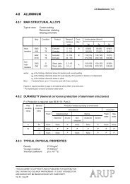
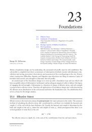
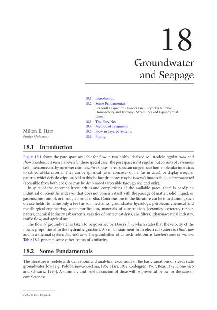
18Groundwaterand SeepageMilton E. HarrPurdue University18.1 Introduction18.2 Some FundamentalsBernoulli’s Equation • Darcy’s Law • Reynolds Number •Homogeneity and Isotropy • Streamlines and EquipotentialLines18.3 The Flow Net18.4 Method of Fragments18.5 Flow in Layered Systems18.6 Piping18.1 IntroductionFigure 18.1 shows the pore space available for flow in two highly idealized soil models: regular cubic andrhombohedral. It is seen that even for these special cases, the pore space is not regular, but consists of cavernouscells interconnected by narrower channels. Pore spaces in real soils can range in size from molecular intersticesto cathedral-like caverns. They can be spherical (as in concrete) or flat (as in clays), or display irregularpatterns which defy description. Add to this the fact that pores may be isolated (inaccessible) or interconnected(accessible from both ends) or may be dead-ended (accessible through one end only).In spite of the apparent irregularities and complexities of the available pores, there is hardly anindustrial or scientific endeavor that does not concern itself with the passage of matter, solid, liquid, orgaseous, into, out of, or through porous media. Contributions to the literature can be found among suchdiverse fields (to name only a few) as soil mechanics, groundwater hydrology, petroleum, chemical, andmetallurgical engineering, water purification, materials of construction (ceramics, concrete, timber,paper), chemical industry (absorbents, varieties of contact catalysts, and filters), pharmaceutical industry,traffic flow, and agriculture.The flow of groundwater is taken to be governed by Darcy’s law, which states that the velocity of theflow is proportional to the hydraulic gradient. A similar statement in an electrical system is Ohm’s lawand in a thermal system, Fourier’s law. The grandfather of all such relations is Newton’s laws of motion.Table 18.1 presents some other points of similarity.18.2 Some FundamentalsThe literature is replete with derivations and analytical excursions of the basic equations of steady stategroundwater flow [e.g., Polubarinova-Kochina, 1962; Harr, 1962; Cedergren, 1967; Bear, 1972; Domenicoand Schwartz, 1990]. A summary and brief discussion of these will be presented below for the sake ofcompleteness.© 2003 by CRC Press LLC

18-2 The Civil Engineering Handbook, Second Edition(a)(b)60°60°(c)90°(d)(e) (f )FIGURE 18.1 Idealized void space.TABLE 18.1Some Similarities of Flow ModelsForm of Energy Name of Law Quantity Storage ResistanceElectrical Ohm’s law Current(voltage)Mechanical Newton’s law Force(velocity)Thermal Fourier’s law Heat flow(temperature)Fluid Darcy’s law Flow rate(pressure)CapacitorMassHeat capacityLiquid storageResistorDamperHeat resistancePermeabilityBernoulli’s EquationUnderlying the analytical approach to groundwater flow is the representation of the actual physical systemby a tractable mathematical model. In spite of their inherent shortcomings, many such analytical modelshave demonstrated considerable success in simulating the action of their prototypes.As is well known from fluid mechanics, for steady flow of nonviscous incompressible fluids, Bernoulli’sequation [Lamb, 1945]----p+ z + ----v 2= constant=g w 2gh(18.1)© 2003 by CRC Press LLC

Groundwater and Seepage 18-3where p = pressure, lb/ft 2g w = unit weight of fluid, lb/ft 3–v = seepage velocity, ft/secg = gravitational constant, 32.2 ft/s 2h = total head, ftdemonstrates that the sum of the pressure head, p/g w , elevation head, z, and velocity head, – v 2 /2g at anypoint within the region of flow is a constant. To account for the loss of energy due to the viscous resistancewithin the individual pores, Bernoulli’s equation is taken as2p A v---- + z AA + ----g w 2g=2p B v---- + z BB + ---- + Dhg w 2g(18.2)where Dh represents the total head loss (energy loss per unit weight of fluid) of the fluid over the distanceDs. The ratioiDh= – lim ----- =D s Æ0Dsdh– -----ds(18.3)is called the hydraulic gradient and represents the space rate of energy dissipation per unit weight of fluid(a pure number).In most problems of interest the velocity heads (the kinetic energy) are so small they can be neglected.For example, a velocity of 1 ft/s, which is large compared to typical seepage velocities through soils,produces a velocity head of only 0.015 ft. Hence, Eq. (18.2) can be simplified top---- A+ z Ag wp---- B+ z B + Dhg wand the total head at any point in the flow domain is simply=h=p---- + zg w(18.4)Darcy’s LawPrior to 1856, the formidable nature of the flow through porous media defied rational analysis. In thatyear, Henry Darcy published a simple relation based on his experiments on the flow of water in verticalsand filters in “Les fontaines publiques de la ville de Dijon,” namely,v = ki = – k dh -----ds(18.5)Equation (18.5), commonly called Darcy’s law, demonstrates a linear dependency between the hydraulicgradient and the discharge velocity v. The discharge velocity, v = nv – , is the product of the porosity n andthe seepage velocity, – v. The coefficient of proportionality k is called by many names depending on itsuse; among these are the coefficient of permeability, hydraulic conductivity, and permeability constant.As shown in Eq. (18.5), k has the dimensions of a velocity. It should be carefully noted that Eq. (18.5)states that flow is a consequence of differences in total head and not of pressure gradients. This isdemonstrated in Fig. 18.2, where the flow is directed from A to B, even though the pressure at point Bis greater than that at point A.© 2003 by CRC Press LLC

18-4 The Civil Engineering Handbook, Second Editionp Ag wA∆hp Bg w∆shBAh Bz Az BFIGURE 18.2 Heads in Bernoulli’s equation.Arbitrary datumTABLE 18.2 Some Typical Values of Coefficientof PermeabilitySoil TypeCoefficient of Permeability k, cm/sClean gravel1.0 and greaterClean sand (coarse) 1.0–0.01Sand (mixtures) 0.01–0.005Fine sand 0.05–0.001Silty sand 0.002–0.0001Silt 0.0005–0.00001Clay0.000001 and smallerDefining Q as the total volume of flow per unit time through a cross-sectional area A, Darcy’s lawtakes the formQ = Av = Aki = – Ak dh -----ds(18.6)Darcy’s law offers the single parameter k to account for both the characteristics of the medium andthe fluid. It has been found that k is a function of g f , the unit weight of the fluid, m, the coefficient ofviscosity, and n, the porosity, as given byk=C g f n--------m(18.7)where C (dimensionally an area) typifies the structural characteristics of the medium independent of thefluid properties. The principal advantage of Eq. (18.7) lies in its use when dealing with more than onefluid or with temperature variations. When employing a single relatively incompressible fluid subjectedto small changes in temperature, such as in groundwater- and seepage-related problems, it is moreconvenient to use k as a single parameter. Some typical values for k are given in Table 18.2.Although Darcy’s law was obtained initially from considerations of one-dimensional macroscopic flow,its practical utility lies in its generalization into two or three spatial dimensions. Accounting for thedirectional dependence of the coefficient of permeability, Darcy’s law can be generalized tohv s = – k ∂s -----∂ s(18.8)© 2003 by CRC Press LLC

Groundwater and Seepage 18-5where k s is the coefficient of permeability in the s direction, and v s and ∂h/∂s are the components of thevelocity and the hydraulic gradient, respectively, in that direction.Reynolds NumberThere remains now the question of the determination of the extent to which Darcy’s law is valid in actualflow systems through soils. Such a criterion is furnished by the Reynolds number R (a pure numberrelating inertial to viscous force), defined asR=vd r---------m(18.9)wherev = discharge velocity, cm/sd = average of diameter of particles, cmr = density of fluid, g(mass)/cm 3m = coefficient of viscosity, g-s/cm 2The critical value of the Reynolds number at which the flow in aggregations of particles changes fromlaminar to turbulent flow has been found by various investigators [see Muskat, 1937] to range between1 and 12. However, it will generally suffice to accept the validity of Darcy’s law when the Reynolds numberis taken as equal to or less than unity, orvd r--------- £ 1m(18.10)Substituting the known values of r and m for water into Eq. (18.10) and assuming a conservativevelocity of 1/4 cm/s, we have d equal to 0.4 mm, which is representative of the average particle size ofcoarse sand.Homogeneity and IsotropyIf the coefficient of permeability is independent of the direction of the velocity, the medium is said tobe isotropic. Moreover, if the same value of the coefficient of permeability holds at all points within theregion of flow, the medium is said to be homogeneous and isotropic. If the coefficient of permeabilitydepends on the direction of the velocity and if this directional dependence is the same at all points ofthe flow region, the medium is said to be homogeneous and anisotropic (or aleotropic).Streamlines and Equipotential LinesPhysically, all flow systems extend in three dimensions. However, in many problems the features of themotion are essentially planar, with the flow pattern being substantially the same in parallel planes. Forthese problems, for steady state, incompressible, isotropic flow in the xy plane, it can be shown [Harr,1962] that the governing differential equation isk x2∂ h ∂ h-------- = k∂ x 2 y -------- = 0∂ y 22(18.11)Here the function h(x, y) is the distribution of the total head (of energy to do work), within and onthe boundaries of a flow region, and k x and k y are the coefficients of permeability in the x and y directions,respectively. If the flow system is isotropic, k x = k y , and Eq. (18.11) reduces to2∂ h ∂ h-------- + -------- = 0∂ x 2∂ y 22(18.12)© 2003 by CRC Press LLC

18-6 The Civil Engineering Handbook, Second EditionEquation (18.12), called Laplace’s equation, is the governing relationship for steady state, laminar-flowconditions (Darcy’s law is valid). The general body of knowledge relating to Laplace’s equation is calledpotential theory. Correspondingly, incompressible steady state fluid flow is often called potential flow. Thecorrespondence is more evident upon the introduction of the velocity potential f, defined asf( x,y) = – kh + C = – kÊ---- p + zˆ+ C˯g w(18.13)where h is the total head, p/g w is the pressure head, z is the elevation head, and C is an arbitrary constant.It should be apparent that, for isotropic conditions,v x=∂------f∂v y = ------f∂ x∂ y(18.14)and Eq. (18.12) will produce— 2 ∂f2 f ∂--------2 f= + -------- = 0∂ x 2∂ y 2(18.15)The particular solutions of Eqs. (18.12) or (18.15) that yield the locus of points within a porousmedium of equal potential, curves along which h(x, y) or f(x, y) are equal to constants, are calledequipotential lines.In analyses of groundwater flow, the family of flow paths is given by the function y(x, y), called thestream function, defined in two dimensions as [Harr, 1962]v x∂ y-------∂ y=v y = – -------∂ y∂ x(18.16)where v x and v y are the components of the velocity in the x and y directions, respectively.Equating the respective potential and stream functions of v x and v y produces∂ f------∂ x=∂ y-------∂ y∂ f------∂ y=∂ y– -------∂ x(18.17)Differentiating the first of these equations with respect to y and the second with respect to x andadding, we obtain Laplace’s equation:∂ 2 y ∂--------2 y+ -------- = 0∂ x 2∂ y 2(18.18)We shall examine the significance of this relationship following a little more discussion of the physicalmeaning of the stream function. Consider AB of Fig. 18.3 as the path of a particle of water passing throughpoint P with a tangential velocity v. We see from the figure thatand hencev yv x--- = tan q =dy-----dxv y dx – v x dy = 0(18.19)© 2003 by CRC Press LLC

Groundwater and Seepage 18-7yBvn yqPn xA0xFIGURE 18.3 Path of flow.Substituting Eq. (18.16), it follows thatwhich states that the total differential d y = 0 andThus we see that the family of curves generated by the function y(x, y) equal to a series of constantsare tangent to the resultant velocity at all points in the flow region and hence define the path of flow.The potential [f = – kh + C] is a measure of the energy available at a point in the flow region to movethe particle of water from that point to the tailwater surface. Recall that the locus of points of equalenergy, say, f(x, y) = constants, are called equipotential lines. The total differential along any curvef(x, y) = constant producesand------- ∂ y∂ xdx ∂ y+ ------- ∂ ydy = 0y ( x,y) = constant∂ f ∂ fdf = ------ dx + ------ dy = 0∂ x ∂ySubstituting for ∂f/∂x and ∂f /∂y from Eqs. (18.16), we havev x dx + v y dy = 0dy-----dx=v– --- xv y(18.20)Noting the negative reciprocal relationship between their slopes, Eqs. (18.19) and (18.20), we see that,within the flow domain, the families of streamlines y (x, y) = constants and equipotential lines f (x, y) =constants intersect each other at right angles. It is customary to signify the sequence of constants byemploying a subscript notation, such as f(x, y) = f i , y(x, y) = y j (Fig. 18.4).As only one streamline may exist at a given point within the flow medium, streamlines cannot intersectone another. Consequently, if the medium is saturated, any pair of streamlines act to form a flow channelbetween them. Consider the flow between the two streamlines y and y + dy in Fig. 18.5; v representsthe resultant velocity of flow. The quantity of flow through the flow channel per unit length normal tothe plane of flow (say, cubic feet per second per foot) isdQ = v x ds cos q – v y ds sin q = v x dy – v y dx =------- ∂ y∂ ydy ∂ y+ ------- dx∂ x© 2003 by CRC Press LLC

18-8 The Civil Engineering Handbook, Second Editiony 1y 2y 3f 1f 2f 3f 4f 5FIGURE 18.4 Streamlines and equipotential lines.yn yynqy + dydxdsqdy0dQn xxFIGURE 18.5 Flow between streamlines.anddQ=dy(18.21)Hence the quantity of flow (also called the discharge quantity) between any pair of streamlines is aconstant whose value is numerically equal to the difference in their respective y values. Thus, once asequence of streamlines of flow has been obtained, with neighboring y values differing by a constantamount, their plot will not only show the expected direction of flow but the relative magnitudes of thevelocity along the flow channels; that is, the velocity at any point in the flow channel varies inverselywith the streamline spacing in the vicinity of that point.An equipotential line was defined previously as the locus of points where there is an expected level ofavailable energy sufficient to move a particle of water from a point on that line to the tailwater surface.Thus, it is convenient to reduce all energy levels relative to a tailwater datum. For example, a piezometerlocated anywhere along an equipotential line, say at 0.75h in Fig. 18.6, would display a column of waterextending to a height of 0.75h above the tailwater surface. Of course, the pressure in the water along theequipotential line would vary with its elevation.0.75 h hTailwaterdatumbaEquipotentialline, 0.75 hFIGURE 18.6 Pressure head along equipotential line.© 2003 by CRC Press LLC

As the quantity of flow between any two streamlines is a constant, DQ, and equal to Dy (Eq. 18.21)we haveEquations (18.22) and (18.23) are approximate. However, as the distances Dw and Ds become verysmall, Eq. (18.22) approaches the velocity at the point and Eq. (18.23) yields the quantity of dischargethrough the flow channel.In Fig. 18.8 is shown the completed flow net for a common type of structure. We first note that thereare four boundaries: the bottom impervious contour of the structure BGHC, the surface of the imperviouslayer EF, the headwater boundary AB, and the tailwater boundary CD. The latter two boundariesdesignate the equipotential lines h = h and h = 0, respectively. For steady state conditions, the quantityGroundwater and Seepage 18-918.3 The Flow NetThe graphical representation of special members of thefamilies of streamlines and corresponding equipotentiallines within a flow region form a flow net. The orthogonal∆QB h + ∆hnetwork shown in Fig. 18.4 represents such a system.Although the construction of a flow net often requires∆shtedious trial-and-error adjustments, it is one of the moreCAvaluable methods employed to obtain solutions for twodimensionaly + ∆ yflow problems. Of additional importance,even a hastily drawn flow net will often provide a check on∆wthe reasonableness of solutions obtained by other means.Noting that, for steady state conditions, Laplace’s equationDalso models the action (see Table 18.1) of thermal, electrical,yacoustical, odoriferous, torsional, and other systems,FIGURE 18.7 Flow at point.the flow net is seen to be a significant tool for analysis.point, according to Darcy’s law, will bek DhDyv ª --------- ª-------Ds D w(18.22)DQ ª k------ DwDhD s(18.23)60 ftA h = 16 ft h = h B50 fth = h 1h 2HGy BGHCC3h = 01Dh 3E2y EFFFIGURE 18.8 Example of flow net.© 2003 by CRC Press LLC

Groundwater and Seepage 18-112h3hh = hAy = 0ah 1h = 0CoarsescreenL3BLy = QCoarsescreenFIGURE 18.9 Example of flow regime.1. Draw the boundaries of the flow region to a scale so that all sketched equipotential lines andstreamlines terminate on the figure.2. Sketch lightly three or four streamlines, keeping in mind that they are only a few of the infinitenumber of possible curves that must provide a smooth transition between the boundary streamlines.3. Sketch the equipotential lines, bearing in mind that they must intersect all streamlines, includingboundary streamlines, at right angles and that the enclosed figures must form curvilinear rectangles(except at singular points) with the same ratio of Ds/Ds along a flow channel. Except for partialflow channels and partial head drops, these will form curvilinear squares with Dw = Ds.4. Adjust the initial streamlines and equipotential lines to meet the required conditions. Rememberthat the drawing of a good flow net is a trial-and-error process, with the amount of correctionbeing dependent upon the position selected for the initial streamlines.Example 18.1Obtain the quantity of discharge, Q/kh, for the section shown in Fig. 18.9.Solution. This represents a region of horizontal flow with parallel horizontal streamlines between theimpervious boundaries and vertical equipotential lines between reservoir boundaries. Hence the flow netwill consist of perfect squares, and the ratio of the number of flow channels to the number of drops willbe N f /N e = a/L and Q/kh = a/L.Example 18.2Find the pressure in the water at points A and B in Fig. 18.9.Solution. For the scheme shown in Fig. 18.9, the total head loss is linear with distance in the directionof flow. Equipotential lines are seen to be vertical. The total heads at points A and B are both equal to2h/3 (datum at the tailwater surface). This means that a piezometer placed at these points would showa column of water rising to an elevation of 2h/3 above the tailwater elevation. Hence, the pressure ateach point is simply the weight of water in the columns above the points in question: p A = (2h/3 + h 1 )g w ,p B = (2h/3 + h l + a)g w .Example 18.3Using flow nets obtain a plot of Q/kh as a function of the ratio s/T for the single impervious sheetpileshown in Fig. 18.10(a).© 2003 by CRC Press LLC

18-12 The Civil Engineering Handbook, Second EditionTshx2.01.5to ∞+b′khQ curve2.01.5y+ d′(a)sT = 0.5N fNe=Qkh1.0+ dQkh curve1.0KhQ(c)sT = 0.80.5+bc+0 0.2 0.4 0.6 0.8 1.0(b)sT = 0.2a0.5sTFIGURE 18.10 Example 18.3.(d ) (e)Solution. We first note that the section is symmetrical about the y axis, hence only one-half of a flownet is required. Values of the ratio s/T range from 0 to 1, with 0 indicating no penetration and 1 completecutoff. For s/T = 1, Q/kh = 0 [see point a in Fig. 18.10(b)]. As the ratio of s/T decreases, more flowchannels must be added to maintain curvilinear squares and, in the limit as s/T approaches zero, Q/khbecomes unbounded [see arrow in Fig. 18.10(b)]. If s/T = 1/2 [Fig. 18.10(c)], each streamline willevidence a corresponding equipotential line in the half-strip; consequently, for the whole flow region,N f /N e = 1/2 for s/T = 1/2 [point b in Fig. 18.10(b)]. Thus, without actually drawing a single flow net, wehave learned quite a bit about the functional relationship between Q/kh and s/T. If Q/kh was known fors/T = 0.8 we would have another point and could sketch, with some reliability, the portion of the plotin Fig. 18.10(b) for s/T ≥ 0.5. In Fig. 18.10(d) is shown one-half of the flow net for s/T = 0.8, which yieldsthe ratio of N f /N e = 0.3 [point c in Fig. 18.10(b)]. As shown in Fig. 18.10(e), the flow net for s/T = 0.8can also serve, geometrically, for the case of s/T = 0.2, which yields approximately N f /N e = 0.8 [plottedas point d in Fig. 18.10(b)]. The portion of the curve for values of s/T close to 0 is still in doubt. Notingthat for s/T = 0, kh/Q = 0, we introduce an ordinate scale of kh/Q to the right of Fig. 18.10(b) and locateon this scale the corresponding values for s/T = 0, 0.2, and 0.5 (shown primed). Connecting these points(shown dotted) and obtaining the inverse, Q/kh, at desired points, the required curve can be had.A plot giving the quantity of discharge (Q/kh) for symmetrically placed pilings as a function of depthof embedment (s/T ), as well as for an impervious structure of width (2b/T ), is shown in Fig. 18.11. Thisplot was obtained by Polubarinova-Kochina [1962] using a mathematical approach. The curve labeledb/T = 0 applies for the conditions in Example 18.3. It is interesting to note that this whole family of© 2003 by CRC Press LLC

Groundwater and Seepage 18-131.51.41.31.2h12Φ1.11.00.90.8Tb b s=Qkh0.70.60.50.40.30.20.10.500.750.251.001.251.50b/T = 0FIGURE 18.11 Quantity of flow for given geometry.0 0.1 0.2 0.3 0.4 0.5 0.6 0.7 0.8 0.9 1.0sTpsIf m = cos tanh 2 πb+ tan2T 2T2 πs2Tfor m ≤ 0.3, Q 1 4kh= pIn mQ −πfor m 2 ≤ 0.9, =kh 1-m2 In( 2)16curves can be obtained, with reasonable accuracy (at least commensurate with the determination of thecoefficient of permeability, k), by sketching only two additional half flow nets (for special values of b/T ).It was tacitly assumed in the foregoing that the medium was homogeneous and isotropic (k x = k y ).Had isotropy not been realized, a transformation of scale (with x and y taken as the directions of maximumand minimum permeability, respectively) in the y direction of Y = y(k x /k y ) 1/2 or in the x direction of X =x(k y /k x ) 1/2 would render the system as an equivalent isotropic system [for details, see Harr, 1962, p. 29].After the flow net has been established, by applying the inverse of the scaling factor, the solution can behad for the anisotropic system. The quantity of discharge for a homogeneous and anisotropic section isQ=k x k y h N f-----N e(18.26)18.4 Method of FragmentsIn spite of its many uses, a graphical flow net provides the solution for a particular problem only. Shouldone wish to investigate the influence of a range of characteristic dimensions (such as is often the case in© 2003 by CRC Press LLC

Groundwater and Seepage 18-15FragmenttypeIllustrationForm factor, Φ (h is headloss through fragment)FragmenttypeIllustrationForm factor, Φ (h is headloss through fragment)ILaΦ =LaVsaLTasL ≤ 2s :LΦ = 2 In (1 + )2aL ≥ 2 s :sΦ = 2 In (1 + ) +aL − 2sTIIIIIIVTTsabAsaEsTbsTbTbTΦ =Φ =1 kh2 Qb ≤ s :Φ = Inb ≥ s :1 kh2 Q( ), Fig. 17.11( ), Fig. 17.11b(1 + )asΦ = In (1 + )a+ b − sTVIVIIVIIIIXs''s'Ta' La''s' 45° 45°s''b'Tb''a''LStreamlineh 1L h 2yha 1d h 1 hαxya 2β h 2 xL ≥ s′ + s′′:s′Φ = In [(1 + ) +a′L − (s′ + s′′)+TQ = k h2 1 − h2 22LhQ = k1 − hIncot αh dh d − hs′′(1 + )]a′′L ≤ s′ + s′′:b′ b′′Φ = In [(1 + )(1 + )]a′ a′′where L + (s′ − s′′)b′ =2L − (s′ − s′′)b′′ =22LΦ =h1 + h 2aQ = k2 a(1 + In2 + h 2)cotβa 2FIGURE 18.14 Summary of fragment types and form factors.andQ=hk------------------mS i = 1Fi(18.28)where h (without subscript) is the total head loss through the section. By similar reasoning, the headloss in the ith fragment can be calculated fromh i=hF--------- iSF(18.29)Thus, the primary task is to implement this method by establishing a catalog of form factors. FollowingPavlovsky, the various form factors will be divided into types. The results are summarized in tabularform, Fig. 18.14, for easy reference. The derivation of the form factors is well documented in the literature[Harr 1962, 1977].Various entrance and emergence conditions for type VIII and IX fragments are shown in Fig. 18.15.Briefly, for the entrance condition, when possible the free surface will intersect the slope at right angles.However, as the elevation of the free surface represents the level of available energy along the uppermoststreamline, at no point along the curve can it rise above the level of its source of energy, the headwaterelevation. At the point of emergence the free surface will, if possible, exit tangent to the slope [Dachler,1934]. As the equipotential lines are assumed to be vertical, there can be only a single value of the totalhead along a vertical line, and, hence, the free surface cannot curve back on itself. Thus, where unableto exit tangent to a slope, it will emerge vertical.To determine the pressure distribution on the base of a structure (such as that along C ¢CC ¢¢) inFig. 18.16, Pavlovsky assumed that the head loss within the fragment is linearly distributed along theimpervious boundary. Thus, in Fig. 18.16, if h m is the head loss within the fragment, the rate of loss alongE¢C ¢CC ¢¢E ¢¢ will be© 2003 by CRC Press LLC

18-16 The Civil Engineering Handbook, Second EditionHorizontalHorizontal90°α α α′α > 90° α = 90° α < 90°(a)TangentβSurfaceof seepageβTangentβVerticalTangenttoverticalβVertical90°β < 90° β = 90° β > 90°(b)FIGURE 18.15 Entrance and emergence conditions.β = 180°DrainC′ CLC′′s′45° F 0E′45°s ′′a′O′NmE′′O′′a′′FIGURE 18.16 Illustration of Eq. (18.30).R=h m-----------------------L+ s¢ + s≤(18.30)Once the total head is known at any point, the pressure can easily be determined by subtracting theelevation head, relative to the established (tailwater) datum.Example 18.4For the section shown in Fig. 18.17(a), estimate (a) the discharge and (b) the uplift pressure on the baseof the structure.Solution. The division of fragments is shown in Fig. 18.17. Regions 1 and 3 are both type II fragments,and the middle section is of type V with L = 2s. For regions 1 and 3, we have, from Fig. 17,11, with b/T =0, F 1 = F 3 = 0.78.For region 2, as L = 2s, F 2 = 2 ln (1+18/36) = 0.81. Thus, the sum of the form factors is F = 0.78 + 0.81 + 0.78 = 2.37and the quantity of flow (Eq. 18.28) is Q/k = 18/2.37 = 7.6 ft.© 2003 by CRC Press LLC

Groundwater and Seepage 18-1718 ft18 ftC′9 ft C C′′9 ftC′ C C′′27 ft1 2 3(a)10.6g w9.0g w7.5g w(b)FIGURE 18.17 Example 18.4.For the head loss in each of the sections, from Eq. (18.29) we find0.78h 1 = h 3 = --------- ( 18 ) = 5.9 ft2.37h 2=6.1ftHence the head loss rate in region 2 is (Eq. 18.30)R6.1= ------ = 17%36and the pressure distribution along C ¢CC ¢¢ is shown in Fig. 18.17(b).Example 18.5 3Estimate the quantity of discharge per foot of structure and the point where the free surface begins underthe structure (point A) for the section shown in Fig. 18.18(a).Solution. The line AC in Fig. 18.18(a) is taken as the vertical equipotential line that separates the flowdomain into two fragments. Region 1 is a fragment of type III, with the distance B as an unknown quantity.Region 2 is a fragment of type VII, with L = 25 – B, h 1 = 10 ft, and h 2 = 0. Thus, we are led to a trial-anderrorprocedure to find B. In Fig. 18.18(b) are shown plots of Q/k versus B/T for both regions. The commonpoint is seen to be B = 14 ft, which yields a quantity of flow of approximately Q = 100k/22 = 4.5k.Example 18.6Determine the quantity of flow for 100 ft of the earth dam section shown in Fig. 18.19(a), where k =0.002 ft/min.Solution. For this case, there are three regions. For region 1, a type VIII fragment h 1 = 70 ft, cot a = 3,h d = 80 ft, producesQ---kFor region 2, a type VII fragment produces70 – h 80= --------------3ln -------------- 80 – h(18.31)Q---k=h 2 2– a--------------- 22L(18.32)3For comparisons between analytical and experimental results for mixed fragments (confined and unconfinedflow) see Harr and Lewis [1965].© 2003 by CRC Press LLC

18-18 The Civil Engineering Handbook, Second Edition8 ftAFree surface(a)10 ftB1 2DrainC25 ftQk8(Q/k) 1(b)642(Q/k) 2B =14 ft0 0.5 1.0 1.5BTFIGURE 18.18 Example 18.5.10 ftyb =20 fta 1a 23020a 2 = 18.3 ftEq. (17.36)h 1 = 70 ft31ah1 2(a)L13b3a 2100x 50h = 52.7 ftEq. (17.38)55 60h(b)FIGURE 18.19 Example 18.6.With tailwater absent, h 2 = 0, the flow in region 3, a type IX fragment, with cot b = 3 producesQ---k=a---- 23(18.33)Finally, from the geometry of the section, we haveL = 20 + cot b [ h d – a 2 ] = 20 + 3 [ 80 – a 2 ](18.34)The four independent equations contain only the four unknowns, h, a 2 , Q/k, and L, and hence providea complete, if not explicit, solution.© 2003 by CRC Press LLC

Groundwater and Seepage 18-19Combining Eqs. (18.32) and (18.33) and substituting for L in Eq. (18.34), we obtain, in general (b =crest width),a 2=----------- b+cot bh – Ê ----------- b +d Ëcotbh d ¯ˆ2– h 2(18.35)and, in particular,20a 2 = ---- + 803Ê20---- + 80 – h 2Ë 3 ¯ˆ2(18.36)Likewise, from Eqs. (18.31) and (18.33), in general,h da ----------------- 2 cot a= (cot bh – h ) ln -------------1 – hh d(18.37)and, in particular,(18.38)Now, Eqs. (18.36) and (18.38), and (18.35) and (18.37) in general, contain only two unknowns (a 2 and h),and hence can be solved without difficulty. For selected values of h, resulting values of a 2 are plotted forEqs. (18.36) and (18.38) in Fig. 18.19(b). Thus, a 2 = 18.3 ft, h = 52.7 ft, and L = 205.1 ft. From Eq. (18.33),the quantity of flow per 100 ft is18.5 Flow in Layered Systems80a 2 = ( 70 – h ) ln-------------- 80 – hQ = 100 ¥ 2 ¥ 10 – 3¥18.3 --------- = 1.22 ft 3 § min = 9.1 gal § min3Closed-form solutions for the flow characteristics of even simple structures founded in layered mediaoffer considerable mathematical difficulty. Polubarinova-Kochina [1962] obtained closed-form solutionsfor the two layered sections shown in Fig. 18.20 (with d 1 = d 2 ). In her solution she found a cluster ofparameters that suggested to Harr [1962] an approximate procedure whereby the flow characteristics ofstructures founded in layered systems can be obtained simply and with a great degree of reliability.hhd 1sBk 1 k 1k 2d 2d 1k 2d 2(a)(b)FIGURE 18.20 Examples of two-layered systems.© 2003 by CRC Press LLC

18-20 The Civil Engineering Handbook, Second EditionThe flow medium in Fig. 18.20(a) consists of two horizontal layers of thickness d 1 and d 2 , underlainby an impervious base. The coefficient of permeability of the upper layer is k 1 and of the lower layer k 2.The coefficients of permeability are related to a dimensionless parameter e by the expressiontan pe =k--- 2k 1(18.39)(p is in radian measure). Thus, as the ratio of the permeabilities varies from 0 to •, e ranges between 0and 1/2. We first investigate the structures shown in Fig. 18.20(a) for some special values of e.1. e = 0. If k 2 = 0, from Eq. (18.39) we have e = 0. This is equivalent to having the impervious baseat depth d 1 . Hence, for this case the flow region is reduced to that of a single homogeneous layerfor which the discharge can be obtained directly from Fig. 18.11.2. e = 1/4. If k 1 = k 2 , the sections are reduced to a single homogeneous layer, of thickness d 1 + d 2 ,for which Fig. 18.11 is again applicable.3. e = 1/2. If k 2 = •, e = 1/2. This represents a condition where there is no resistance to flow in thebottom layer. Hence, the discharge through the total section under steady state conditions isinfinite, or Q/k 1 h = •. However, of greater significance is the fact that the inverse of this ratioequals zero: k 1 h/Q = 0. It can be shown [Polubarinova-Kochina, 1962] that for k 2 /k 1 Æ •,Q-------k 1 h=k--- 2k 1(18.40)Thus, we see that for the special values of e = 0, e = 1/4, and e = 1/2, measures of the flow quantitiescan be easily obtained. The essence of the method then is to plot these values, on a plot of k 1 h/Q versuse, and connect the points with a smooth curve, from which intermediate values can be had.Example 18.7In Fig. 18.20(a), s = 10 ft, d 1 = 15 ft, d 2 = 20 ft, k 1 = 4k 2 = 1 • 10 –3 ft/min, h = 6 ft. Estimate Q/k 1 h.Solution. For e = 0, from Fig. 18.11 with s/T = s/d 1 = 2/3, b/T = 0, Q/k 1 h = 0.39, k 1 h/Q = 2.56.For e = 1/4, from Fig. 18.11 with s/T = s/(d 1 + d 2 ) = 2/7, Q/k 1 h = 0.67, k 1 h/Q = 1.49.For e = 1/2, k 1 h/Q = 0.The three points are plotted in Fig. 18.21, and the required discharge, for e = 1/p tan –1 . (1/4) 1/2 = 0.15,is k 1 h/Q = 1.92 and Q/k 1 h = 0.52; whenceQ = 0.52 ¥ 1 ¥ 10 – 3¥ 6= 3.1 ¥ 10 – 3ft 3 § ( min)( ft)In combination with the method of fragments, approximate solutions can be had for very complicatedstructures.Example 18.8Estimate (a) the discharge through the section shown in Fig. 18.22(a), k 2 = 4k 1 = 1 ¥ 10 –3 ft/day and(b) the pressure in the water at point P.Solution. The flow region is shown divided into four fragments. However, the form factors for regions 1and 4 are the same. In Fig. 18.22(b) are given the resulting form factors for the listed conditions. InFig. 18.22(c) is given the plot of k 1 h/Q versus e. For the required condition (k 2 = 4k 1 ), e = 0.35, k 1 h/Q =1.6 and hence Q = (1/1.6) ¥ 0.25 ¥ 10 –3 ¥ 10 = 1.6 ¥ 10 –3 ft 3 /(day) (ft).The total head at point P is given in Fig. 18.22(b) as Dh for region 4; for e = 0, h p = 2.57 ft and fore = 1/4, h p = 3.00. We require h p for k 2 = •; theoretically, there is assumed to be no resistance to the flow© 2003 by CRC Press LLC

Groundwater and Seepage 18-213tan p =k 2k 121.92k h 1Q100.15 0.25 0.50FIGURE 18.21 Example 18.7.in the bottom layer for this condition. Hence the boundary between the two layers (AB) is an equipotentialline with an expected value of h/2. Thus h p = 10/2 = 5 for e = 1/2. In Fig. 18.22(d) is given the plot ofh p versus e. For e = 0.35, h p = 2.75 ft and the pressure in the water at point P is (3.75 + 5)g w = 8.75g w .The above procedure may be extended to systems with more than two layers.18.6 PipingBy virtue of the viscous friction exerted on a liquid flowing through a porous medium, an energy transferis effected between the liquid and the solid particles. The measure of this energy is the head loss h betweenthe points under consideration. The force corresponding to this energy transfer is called the seepage force.It is this seepage force that is responsible for the phenomenon known as quicksand, and its assessmentis of vital importance in stability analyses of earth structures subject to the action of flowing water(seepage).The first rational approach to the determination of the effects of seepage forces was presented byTerzaghi [1922] and forms the basis for all subsequent studies. Consider all the forces acting on a volumeof particulate matter through which a liquid flows.1. The total weight per unit volume, the mass unit weight, isgg 1 ( G+e)m = ----------------------1 + ewhere e is the void ratio, G is the specific gravity of solids, and g l is the unit weight of the liquid.2. Invoking Archimedes’ principle of buoyancy (a body submerged in a liquid is buoyed up by forceequal to the weight of the liquid displaced), the effective unit weight of a volume of soil, calledthe submerged unit weight, isg m ¢ = g m – g l =g l ( G – 1 )----------------------1 + e(18.41)To gain a better understanding of the meaning of the submerged unit weight consider the flowcondition shown in Fig. 18.23(a). If the water column (AB) is held at the same elevation as thedischarge face CD (h = 0), the soil will be in a submerged state and the downward force actingon the screen will beFØ = g ¢ m LA(18.42)© 2003 by CRC Press LLC

18-22 The Civil Engineering Handbook, Second Edition10 ft5 ft13 ft 13 ftk 115 ft1 2 3 4A15 ftk 2BRegion1 II 0.96 0.74 2.57 3.002TypeV = 01.02 = 1 40.58∆ h = 02.73∆ h1 =42.363I0.800.402.141.63(a)4II0.960.742.573.004ΣΦ3.742.46Check:10.0Check:10.0(b)3h pk 1 hQ = ΣΦ21.6651433.750.250.350.5021(c)0.250.350.5(d )FIGURE 18.22 Example 18.8.where g¢ m = g m – g w . Now, if the water column is slowly raised (shown dotted to A¢B¢), water willflow up through the soil. By virtue of this upward flow, work will be done to the soil and the forceacting on the screen will be reduced.3. The change in force through the soil is due to the increased pressure acting over the area, orF +=hg w AHence, the change in force, granted steady state conditions, isDF= g ¢ m LA – hg w A(18.43)© 2003 by CRC Press LLC

Groundwater and Seepage 18-23A′ B′ABC hD(b)g m ′RWatercolumnLMaterialArea, AScreen(c)g m ′Riγ wiγ w(a)FIGURE 18.23 Piping.isDividing by the volume AL, the resultant force per unit volume acting at a point within the flow regionR = g ¢ m– ig w(18.44)where i is the hydraulic gradient. The quantity i g w is the seepage force (force per unit volume). In general,Eq. (18.44) is a vector equation, with the seepage force acting in the direction of flow [Fig. 18.23(b)]. Ofcourse, for the flow condition shown in Fig. 18.23(a), the seepage force will be directed vertically upward[Fig. 18.23(c)].If the head h is increased, the resultant force R in Eq. (18.44) is seen to decrease. Evidently, should hbe increased to the point at which R = 0, the material would be at the point of being washed upward.Such a state is said to produce a quick (meaning alive) condition. From Eq. (18.44) it is evident that aquick condition is incipient ifgi m¢cr = ----- =g wG – 1------------1 + e(18.45)Substituting typical values of G = 2.65 (quartz sand) and e = 0.65 (for sand, 0.57 £ e £ 0.95), we seethat as an average value the critical gradient can be taken asi cr ª 1(18.46)When information is lacking as to the specific gravity and void ratio of the material, the critical gradientis generally taken as unity.At the critical gradient, there is no interparticle contact (R = 0); the medium possesses no intrinsicstrength, and will exhibit the properties of liquid of unit weightG+eg q = Ê------------ˆ gË1 + e ¯ l(18.47)Substituting the above values for G, e, and g l = g w , g q = 124.8 lb/ft 3 . Hence, contrary to popular belief,a person caught in quicksand would not be sucked down but would find it almost impossible to avoidfloating.© 2003 by CRC Press LLC

18-24 The Civil Engineering Handbook, Second Edition1.0E0.8sh mT0.6l sEh m0.40.20s/T0.2 0.4 0.6 0.8 1.0FIGURE 18.24 Exit gradient.Many hydraulic structures, founded on soils, have failed as a result of the initiation of a local quickcondition which, in a chainlike manner, led to severe internal erosion called piping. This condition occurswhen erosion starts at the exit point of a flow line and progresses backward into the flow region formingpipe-shaped watercourses which may extend to appreciable depths under a structure. It is characteristicof piping that it needs to occur only locally and that once begun it proceeds rapidly, and is often notapparent until structural failure is imminent.Equations (18.45) and (18.46) provide the basis for assessing the safety of hydraulic structures withrespect to failure by piping. In essence, the procedure requires the determination of the maximumhydraulic gradient along a discharge boundary, called the exit gradient, which will yield the minimumresultant force (R min ) at this boundary. This can be done analytically, as will be demonstrated below, orfrom flow nets, after a method proposed by Harza [1935].In the graphical method, the gradients along the discharge boundary are taken as the macrogradientacross the contiguous squares of the flow net. As the gradients vary inversely with the distance betweenadjacent equipotential lines, it is evident that the maximum (exit) gradient is located where the verticalprojection of this distance is a minimum, such as at the toe of the structure (point C) in Fig. 18.11. Forexample, the head lost in the final square of Fig. 18.11 is one-sixteenth of the total head loss of 16 ft, or1 ft, and as this loss occurs in a vertical distance of approximately 4 ft, the exit gradient at point C isapproximately 0.25. Once the magnitude of the exit gradient has been found, Harza recommended thatthe factor of safety be ascertained by comparing this gradient with the critical gradient of Eqs. (18.45)and (18.46). For example, the factor of safety with respect to piping for the flow conditions of Fig. 18.11is 1.0/0.25, or 4.0. Factors of safety of 4 to 5 are generally considered reasonable for the graphical methodof analysis.The analytical method for determining the exit gradient is based on determining the exit gradient forthe type II fragment, at point E in Fig. 18.14. The required value can be obtained directly from Fig. 18.24with h m being the head loss in the fragment.Example 18.9Find the exit gradient for the section shown in Fig. 18.17(a).Solution. From the results of Example 18.4, the head loss in fragment 3 is h m = 5.9 ft. With s/T = 1/3,from Fig. 18.24 we have I E s/h m = 0.62; hence,© 2003 by CRC Press LLC

Groundwater and Seepage 18-25To account for the deviations and uncertainties in nature, Khosla et al. [1954] recommend that thefollowing factors of safety be applied as critical values of exit gradients: gravel, 4 to 5; coarse sand, 5 to6; and fine sand, 6 to 7.The use of reverse filters on the downstream surface or where required serves to prevent erosion anddecrease the probability of piping failures. In this regard, the Earth Manual of the U.S. Bureau ofReclamation, Washington [1974] is particularly recommended.Defining TermsCoefficient of permeability — Coefficient of proportionality between Darcy’s velocity and the hydraulicgradient.Flow net — Trial-and-error graphical procedure for solving seepage problems.Hydraulic gradient — Space rate of energy dissipation.Method of fragments — Approximate analytical method for solving seepage problems.Piping — Development of a “pipe” within soil by virtue of internal erosion.Quick condition — Condition when soil “liquifies.”References0.62 ¥ 5.91I E = ---------------------- = 0.41 or FS = --------- = 2.4490.41Bear, J. 1972. Dynamics of Fluids in Porous Media. American Elsevier, New York.Bear, J., Zaslavsky, D., and Irmay, S. 1966. Physical Principles of Water Percolation and Seepage. Technion,Israel.Brahma, S. P., and Harr, M. E. 1962. Transient development of the free surface in a homogeneous earthdam. Geotechnique. 12(4).Casagrande, A. 1940. Seepage Through Dams. In Contributions to Soil Mechanics 1925–1940. BostonSociety of Civil Engineering, Boston.Cedergren, H. R. 1967. Seepage, Drainage and Flow Nets. John Wiley & Sons, New York.Dachler, R. 1934. Ueber den Strömungsvorgang bei Hanquellen. Die Wasserwirtschaft, no. 5.Darcy, H. 1856. Les Fontaines publique de la ville de Dijon. Paris.Domenico, P. A., and Schwartz, F. W. 1990. Physical and Chemical Hydrogeology. John Wiley & Sons, NewYork.Dvinoff, A. H., and Harr, M. E. 1971. Phreatic surface location after drawdown. J. Soil Mech. Found.ASCE. January.Earth Manual. 1974. Water Resources Technology Publication, 2nd ed. U.S. Department of Interior, Bureauof Reclamation, Washington, D.C.Forchheimer, P. 1930. Hydraulik. Teubner Verlagsgesellschaft, Stuttgart.Freeze, R. A., and Cherry, J. A. 1979. Groundwater. Prentice-Hall, Englewood Cliffs, NJ.Harr, M. E. 1962. Groundwater and Seepage. McGraw-Hill, New York.Harr, M. E., and Lewis, K. H. 1965. Seepage around cutoff walls. RILEM, Bulletin 29, December.Harr, M. E. 1977. Mechanics of Particulate Media: A Probabilistic Approach. McGraw-Hill, New York.Harza, L. F. 1935. Uplift and seepage under dams on sand. Trans. ASCE, vol. 100.Khosla, R. B. A. N., Bose, N. K., and Taylor, E. M. 1954. Design of Weirs on Permeable Foundations. CentralBoard of Irrigation, New Delhi, India.Lambe, H. 1945. Hydrodynamics. Dover, New York.Muskat, M. 1937. The Flow of Homogeneous Fluids through Porous Media. McGraw-Hill, New York.Reprinted by J. W. Edwards, Ann Arbor, 1946.Pavlovsky, N. N. 1956. Collected Works. Akad. Nauk USSR, Leningrad.Polubarinova-Kochina, P. Ya. 1941. Concerning seepage in heterogeneous (two-layered) media. InzhenerniiSbornik. 1(2).© 2003 by CRC Press LLC

18-26 The Civil Engineering Handbook, Second EditionPolubarinova-Kochina, P. Ya. 1962. Theory of the Motion of Ground Water. Translated by J. M. R. De Wiest.Princeton University Press, Princeton, New Jersey. (Original work published 1952.)Prasil, F. 1913. Technische Hydrodynamik. Springer-Verlag, Berlin.Scheidegger, A. E. 1957. The Physics of Flow through Porous Media. Macmillan, New York.Terzaghi, K. 1922. Der Grundbruch and Stauwerken und seine Verhütung. Die Wasserkraft, p. 445.Further InformationThis chapter dealt with the conventional analysis of groundwater and seepage problems. Beginning inthe mid-1970s another facet was added, motivated by federal environmental laws. These were concernedwith transport processes, where chemical masses, generally toxic, are moved within the groundwaterregime. This aspect of groundwater analysis gained increased emphasis with the passage of the ComprehensiveEnvironmental Response Act of 1980, the superfund. Geotechnical engineers’ involvement inthese problems is likely to overshadow conventional problems. Several of the above references providespecific sources of information in this regard (cf. Domenico and Schwartz, Freeze and Cherry). Thefollowing are of additional interest:Bear, J., and Verruijt, A. 1987. Modeling Groundwater Flow and Pollution. Dordrecht, Boston: D. ReidelPub. Co., Norwell, MA.Mitchell, J. K. 1993. Fundamentals of Soil Behavior. John Wiley & Sons, New York.Nyer, E. K. 1992. Groundwater Treatment Technology. Van Nostrand Reinhold, New York.Sara, M. N. 1994. Standard Handbook for Solid and Hazardous Waste Facility Assessments. Lewis Publishers,Boca Raton, FL.© 2003 by CRC Press LLC