The Heisenberg Antiferromagnet and the Lanczos Algorithm Abstract

More documents

Recommendations

Info

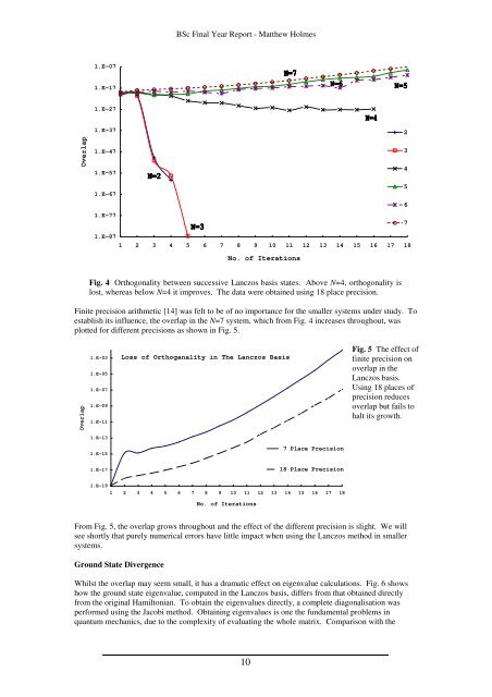
BSc Final Year Report - Matthew Holmes1.E-071.E-171.E-27Overlap1.E-371.E-471.E-571.E-671.E-772345671.E-871 2 3 4 5 6 7 8 9 10 11 12 13 14 15 16 17 18No. of IterationsFig. 4 Orthogonality between successive Lanczos basis states. Above N=4, orthogonality islost, whereas below N=4 it improves. The data were obtained using 18 place precision.Finite precision arithmetic [14] was felt to be of no importance for the smaller systems under study. Toestablish its influence, the overlap in the N=7 system, which from Fig. 4 increases throughout, wasplotted for different precisions as shown in Fig. 5.Overlap1.E-031.E-051.E-071.E-091.E-11Loss of Orthoganality in The Lanczos BasisFig. 5 The effect offinite precision onoverlap in theLanczos basis.Using 18 places ofprecision reducesoverlap but fails tohalt its growth.1.E-131.E-157 Place Precision1.E-1718 Place Precision1.E-191 2 3 4 5 6 7 8 9 10 11 12 13 14 15 16 17 18No. of IterationsFrom Fig. 5, the overlap grows throughout and the effect of the different precision is slight. We willsee shortly that purely numerical errors have little impact when using the Lanczos method in smallersystems.Ground State DivergenceWhilst the overlap may seem small, it has a dramatic effect on eigenvalue calculations. Fig. 6 showshow the ground state eigenvalue, computed in the Lanczos basis, differs from that obtained directlyfrom the original Hamiltonian. To obtain the eigenvalues directly, a complete diagonalisation wasperformed using the Jacobi method. Obtaining eigenvalues is one the fundamental problems inquantum mechanics, due to the complexity of evaluating the whole matrix. Comparison with the10
BSc Final Year Report - Matthew HolmesJacobi results are for illustrative purposes and, in general, methods such as the Lanczos schemeconsidered here are preferred, and often essential.The ground state energy should be roughly linear with N [7]. Our direct evaluation is reassuringly ontrack. The observed divergence of the Lanczos values however, requires further analysis. Theinfluence of finite precision is also seen to be negligible.Ground State Energy, J0-10-20-30Original Hamiltonian-40 Lanczos Hamiltonian: 18 Place PrecisionLanczos Hamiltonian: 7 Place Precision-502 3 4 5 6 7System Size, NFig. 6 Divergence ofthe ground stateenergies. If overlapis ignored, the valuescomputed from theLanczos matrixbegin, very quickly,to diverge from thetrue ground states.The N=4 estimate is~0.1J in error for 18place precision,where J are units ofexchange energy.The negligibleinfluence of finiteprecision arithmeticis clear.If accurate eigenstates are to be obtained, the overlap must improve. Simply increasing the precision isinsufficient. Another option is to suspend the procedure when the overlap becomes too large. We thenuse the current eigenvalue of interest k to construct a new vector, with greater projection along thedesired state, with which to restart the procedure. The flow scheme below shows how this may beimplemented.DO1. Start with normalised vector, v 12. Find next state v 23. Calculate eigenvalues andeigenvectors of current matrix4. Calculate overlap5. If overlap > then build new v 1 from k and cycle to 1.Fig. 7 Flow scheme forevolving the Lanczosbasis whilst maintainingorthogonality.We terminate before theoverlap reaches , thevalue at whichunacceptable errorsappear. Using the currenteigenvalue of interest k anew vector v 1 isconstructed for restartingthe procedure.DO until: new k ~ old kWe need not store the Lanczos basis [19,13], when running the procedure. If step 5 of Fig. 7, isrequired, we select f k (the kth column of the transformation matrix found in step 3) corresponding to k .f k is then used to initiate a separate run, building a new starting vector v 1 for step 1. of Fig. 7.The Variational Approach: Modified LanczosThe idea just introduced may be taken to its extreme by continually restarting after just one iteration[13,12]. In this way we only ever evaluate 2x2 matrices and the current ground state is always in thememory. This approach, known as the modified Lanczos method, is a variational technique [8].Although more pedestrian than the regular routine [13], for smaller systems it is convenient foreliminating overlap, confining it to ~10 -20 for all system sizes. Fig. 8 shows how this effects the groundstate calculations.11
Page 1 and 2: The Heisenberg Antiferromagnet and
Page 3 and 4: BSc Final Year Report - Matthew Hol
Page 9: BSc Final Year Report - Matthew Hol
Page 17: BSc Final Year Report - Matthew Hol

The Heisenberg Antiferromagnet and the Lanczos Algorithm Abstract

You also want an ePaper? Increase the reach of your titles

Delete template?

Save as template?