Graphics with PGF and TikZ - TUG

Graphics with PGF and TikZ
Andrew Mertz, William Slough
Department of Mathematics and Computer Science
Eastern Illinois University
Charleston, IL 61920
aemertz (at) eiu dot edu, waslough (at) eiu dot edu
1 Introduction
Abstract
Beautiful and expressive documents often require beautiful and expressive graphics.
PGF and its front-end TikZ walk a fine line between power, portability and
usability, giving a TEX-like approach to graphics. While PGF and TikZ are extensively
documented, first-time users may prefer learning about these packages
using a collection of graduated examples. The examples presented here cover a
wide spectrum of use and provide a starting point for exploration.
Users of TEX and L ATEX intending to create and use
graphics within their documents have a multitude
of choices. For example, the UK TEX FAQ [1] lists
a half dozen systems in its response to “Drawing
with TEX”. One of these systems is PGF and its
associated front-end, TikZ [4].
All of these systems have similar goals: namely,
to provide a language-based approach which allows
for the creation of graphics which blend well with
TEX and L ATEX documents. This approach stands
in contrast to the use of an external drawing program,
whose output is subsequently included in the
document using the technique of graphics inclusion.
PGF provides a collection of low-level graphics
primitives whereas TikZ is a high-level user interface.
Our intent is to provide an overview of the
capabilities of TikZ and to convey a sense of both
its power and relative simplicity. The examples used
here have been developed with Version 1.0 of TikZ.
2 The name of the game
Users of TEX are accustomed to acronyms; both
PGF and TikZ follow in this tradition. PGF refers
to Portable Graphics Format. In a tip of the hat to
the recursive acronym GNU (i.e., GNU’s not Unix),
TikZ stands for “TikZ ist kein Zeichenprogramm”,
a reminder that TikZ is not an interactive drawing
program.
3 Getting started
TikZ supports both plain TEX and L ATEX input formats
and is capable of producing PDF, PostScript,
and SVG outputs. However, we limit our discussion
to one choice: L ATEX input, with PDF output, processed
by pdfL ATEX.
TikZ provides a one-step approach to adding
graphics to a L ATEX document. TikZ commands
which describe the desired graphics are simply intermingled
with the text. Processing the input source
yields the PDF output.
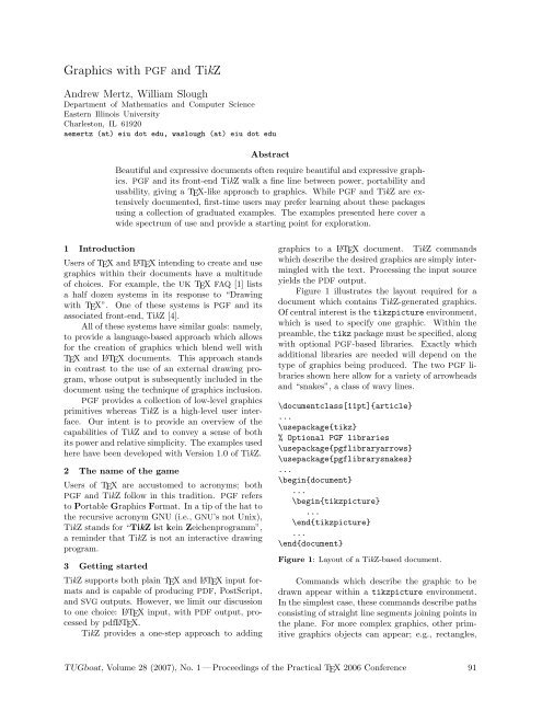
Figure 1 illustrates the layout required for a
document which contains TikZ-generated graphics.
Of central interest is the tikzpicture environment,
which is used to specify one graphic. Within the
preamble, the tikz package must be specified, along
with optional PGF-based libraries. Exactly which
additional libraries are needed will depend on the
type of graphics being produced. The two PGF libraries
shown here allow for a variety of arrowheads
and “snakes”, a class of wavy lines.
\documentclass[11pt]{article}
...
\usepackage{tikz}
% Optional PGF libraries
\usepackage{pgflibraryarrows}
\usepackage{pgflibrarysnakes}
...
\begin{document}
...
\begin{tikzpicture}
...
\end{tikzpicture}
...
\end{document}
Figure 1: Layout of a TikZ-based document.
Commands which describe the graphic to be
drawn appear within a tikzpicture environment.
In the simplest case, these commands describe paths
consisting of straight line segments joining points in
the plane. For more complex graphics, other primitive
graphics objects can appear; e.g., rectangles,
TUGboat, Volume 28 (2007), No. 1 — Proceedings of the Practical TEX 2006 Conference 91

Andrew Mertz, William Slough
\begin{tikzpicture}
\draw (1,0) -- (0,1) -- (-1,0) -- (0,-1) -- cycle;
\end{tikzpicture}
Figure 2: Drawing a diamond with a closed path.
\begin{tikzpicture}
\draw[step=0.25cm,color=gray] (-1,-1) grid (1,1);
\draw (1,0) -- (0,1) -- (-1,0) -- (0,-1) -- cycle;
\end{tikzpicture}
Figure 3: Adding a grid.
circles, arcs, text, grids, and so forth.
Figure 2 illustrates how a diamond can be obtained,
using the draw command to cause a “pen”
to form a closed path joining the four points (1, 0),
(0, 1), (−1, 0), and (0, −1), specified with familiar
Cartesian coordinates. The syntax used to specify
this path is very similar to that used by Meta-
Post [2]. Unlike MetaPost, TikZ uses one centimeter
as the default unit of measure, so the four points
used in this example lie on the x and y axes, one
centimeter from the origin.
In the process of developing and “debugging”
graphics, it can be helpful to include a background
grid. Figure 3 expands on the example of Figure 2 by
adding a draw command to cause a grid to appear:
\draw[step=0.25cm,color=gray]
(-1,-1) grid (1,1);
In this command, the grid is specified by providing
two diagonally opposing points: (−1, −1) and (1, 1).
The two options supplied give a step size for the grid
lines and a specification for the color of the grid lines,
using the xcolor package [3].
4 Specifying points and paths in TikZ
Two key ideas used in TikZ are points and paths.
Both of these ideas were used in the diamond examples.
Much more is possible, however. For example,
points can be specified in any of the following ways:
• Cartesian coordinates
• Polar coordinates
• Named points
• Relative points
As previously noted, the Cartesian coordinate
(a, b) refers to the point a centimeters in the xdirection
and b centimeters in the y-direction.
A point in polar coordinates requires an angle
α, in degrees, and distance from the origin, r. Unlike
Cartesian coordinates, the distance does not have a
default dimensional unit, so one must be supplied.
The syntax for a point specified in polar coordinates
is (α : r dim), where dim is a dimensional unit such
as cm, pt, in, or any other TEX-based unit. Other
than syntax and the required dimensional unit, this
follows usual mathematical usage. See Figure 4.
y
Figure 4: Polar coordinates in TikZ.
α
r
(α : r dim)
It is sometimes convenient to refer to a point by
name, especially when this point occurs in multiple
\draw commands. The command:
\path (a,b) coordinate (P);
assigns to P the Cartesian coordinate (a, b). In a
similar way,
\path (α:r dim) coordinate (Q);
assigns to Q the polar coordinate with angle α and
radius r.
Figure 5 illustrates the use of named coordinates
and several other interesting capabilities of
TikZ. First, infix-style arithmetic is used to help define
the points of the pentagon by using multiples
of 72 degrees. This feature is made possible by the
calc package [5], which is automatically included by
TikZ. Second, the \draw command specifies five line
segments, demonstrating how the drawing pen can
be moved by omitting the -- operator.
92 TUGboat, Volume 28 (2007), No. 1 — Proceedings of the Practical TEX 2006 Conference
x

\begin{tikzpicture}
% Define the points of a regular pentagon
\path (0,0) coordinate (origin);
\path (0:1cm) coordinate (P0);
\path (1*72:1cm) coordinate (P1);
\path (2*72:1cm) coordinate (P2);
\path (3*72:1cm) coordinate (P3);
\path (4*72:1cm) coordinate (P4);
% Draw the edges of the pentagon
\draw (P0) -- (P1) -- (P2) -- (P3) -- (P4) -- cycle;
% Add "spokes"
\draw (origin) -- (P0) (origin) -- (P1) (origin) -- (P2)
(origin) -- (P3) (origin) -- (P4);
\end{tikzpicture}
Figure 5: Using named coordinates.
P
∆x
Q
∆y
Figure 6: A relative point, Q, determined with Cartesian
or polar offsets.
The concept of the current point plays an important
role when multiple actions are involved. For
example, suppose two line segments are drawn joining
points P and Q along with Q and R:
P
\draw (P) -- (Q) -- (R);
Viewed as a sequence of actions, the drawing pen
begins at P , is moved to Q, drawing a first line segment,
and from there is moved to R, yielding a second
line segment. As the pen moves through these
two segments, the current point changes: it is initially
at P , then becomes Q and finally becomes R.
A relative point may be defined by providing
offsets in each of the horizontal and vertical directions.
If P is a given point and ∆x and ∆y are two
offsets, a new point Q may be defined using a ++
prefix, as follows:
\path (P) ++(∆x,∆y) coordinate (Q);
Alternately, the offset may be specified with polar
coordinates. For example, given angle α and radius
r, with a dimensional unit dim, the command:
\path (P) ++(α:r dim) coordinate (Q);
specifies a new point Q. See Figure 6.
There are two forms of relative points — one
which updates the current point and one which does
r
α
Q
Graphics with PGF and TikZ
not. The ++ prefix updates the current point while
the + prefix does not.
Consider line segments drawn between points
defined in a relative manner, as in the example of
Figure 7. The path is specified by offsets: the drawing
pen starts at the origin and is adjusted first by
the offset (1, 0), followed by the offset (1, 1), and
finally by the offset (1, −1).
By contrast, Figure 8 shows the effect of using
the + prefix. Since the current point is not updated
in this variation, every offset which appears is performed
relative to the initial point, (0, 0).
Beyond line segments
In addition to points and line segments, there are a
number of other graphic primitives available. These
include:
• Grids and rectangles
• Circles and ellipses
• Arcs
• Bézier curves
As previously discussed, a grid is specified by providing
two diagonally opposing points and other options
which affect such things as the color and spacing
of the grid lines. A rectangle can be viewed as
a simplified grid — all that is needed are two diagonally
opposing points of the rectangle. The syntax
\draw (P) rectangle (Q);
draws the rectangle specified by the two “bounding
box” points P and Q. It is worth noting that the
current point is updated to Q, a fact which plays a
role if the \draw command involves more than one
drawing action. Figure 9 provides an example where
TUGboat, Volume 28 (2007), No. 1 — Proceedings of the Practical TEX 2006 Conference 93

Andrew Mertz, William Slough
\begin{tikzpicture}
\draw (0,0) -- ++(1,0) -- ++(1,1) -- ++(1,-1);
\end{tikzpicture}
Figure 7: Drawing a path using relative offsets.
\begin{tikzpicture}
\draw (0,0) -- +(1,0) -- +(0,-1) -- +(-1,0) -- +(0,1);
\end{tikzpicture}
Figure 8: Drawing a path using relative offsets without updating the current point.
\begin{tikzpicture}
\draw (0,0) rectangle (1,1)
rectangle (3,2)
rectangle (4,3);
\end{tikzpicture}
Figure 9: Drawing rectangles.
\begin{tikzpicture}
\draw (0,0) circle (1cm)
circle (0.6cm)
circle (0.2cm);
\end{tikzpicture}
Figure 10: Drawing circles — one draw command with multiple actions.
\begin{tikzpicture}
\draw (0,0) circle (1cm);
\draw (0.5,0) circle (0.5cm);
\draw (0,0.5) circle (0.5cm);
\draw (-0.5,0) circle (0.5cm);
\draw (0,-0.5) circle (0.5cm);
\end{tikzpicture}
Figure 11: Drawing circles — a sequence of draw commands.
three rectangles are drawn in succession. Each rectangle
operation updates the current point, which
then serves as one of the bounding box points for
the following rectangle.
A circle is specified by providing its center point
and the desired radius. The command:
\draw (a,b) circle (r dim);
causes the circle with radius r, with an appropriate
dimensional unit, and center point (a, b) to be
drawn. The current point is not updated as a result.
Figures 10 and 11 provide examples.
The situation for an ellipse is similar, though
two radii are needed, one for each axis. The syntax:
\draw (a,b) ellipse (r1 dim and r2 dim);
causes the ellipse centered at (a, b) with semi-axes
y
b
r2
Figure 12: An ellipse in TikZ.
94 TUGboat, Volume 28 (2007), No. 1 — Proceedings of the Practical TEX 2006 Conference
a
r1
x

\begin{tikzpicture}
\draw (0,0) ellipse (2cm and 1cm)
ellipse (0.5cm and 1 cm)
ellipse (0.5cm and 0.25cm);
\end{tikzpicture}
Figure 13: Three ellipses produced with a single draw command.
Figure 14: An arc in TikZ.
r
\begin{tikzpicture}
\draw (0:0.7cm) -- (0:1.5cm)
arc (0:60:1.5cm) -- (60:0.7cm)
arc (60:0:0.7cm) -- cycle;
\end{tikzpicture}
Figure 15: Combining arcs and line segments.
y
β
C D
P Q
Figure 16: A Bézier curve.
α
P
x
Graphics with PGF and TikZ
r1 and r2 to be drawn. See Figure 12. Like circle,
the ellipse command does not change the current
point, so multiple ellipses which share the same center
point can be drawn with a single draw command,
as Figure 13 shows.
Arcs may also be specified in TikZ. For a circular
arc, what is required is an initial point on the
circle, the radius of the circle and an indication of
how much of the circle to be swept out. In more
detail, the syntax
\draw (P ) arc (α:β:r dim);
draws the arc shown in Figure 14. At first glance
it might seem unusual to use the point P and not
the center point of the circle. However, when one
realizes that the arc might be just one of several
components of a draw command, it is very natural
to use the point P , as it will be the current point.
For example, Figure 15 shows how to draw a
portion of an annulus by drawing two arcs and two
line segments. This particular figure is drawn by
directing the pen in a counter-clockwise fashion—
the horizontal line segment, the outer circular arc,
a line segment, and finally the inner arc.
TikZ also provides the ability to produce Bézier
curves. The command
\draw (P ) .. controls (C)
and (D) .. (Q);
draws the curve shown in Figure 16. Four points are
needed: an initial point P , a final point Q, and two
control points. The location of the control points
controls the extent of the curve and the slope of the
curve at the initial and final points.
Bézier curves provide for a wealth of variety, as
Figure 17 indicates.
An alternate syntax for Bézier curves allows for
a more convenient specification of the curvature at
the starting and ending points. Using polar coordinates
with respect to these two points provides this
capability. The syntax is as follows:
\draw (P ) .. controls +(α:r1 dim)
and +(β:r2 dim) .. (Q);
See Figure 18.
TUGboat, Volume 28 (2007), No. 1 — Proceedings of the Practical TEX 2006 Conference 95

Andrew Mertz, William Slough
Figure 17: Various Bézier curves.
r1
C D
P Q
C D
P Q
α
P Q
Figure 18: A Bézier curve specified with relative coordinates.
5 From coordinates to nodes
A node is a generalization of the coordinate primitive.
Two characteristics of a node are its shape and
its text. A node allows for arbitrary TEX text to
appear within a diagram. The command
\path (0,0)
node[draw,shape=circle] (v0)
{$v_0$};
defines a node named v0, centered at the origin,
with a circular shape and text component $v_0$.
The draw option causes the associated shape (in
this case, a circle) to be drawn. Figure 19 illustrates
how nodes can be used to draw an undirected graph.
Notice how line segments which join nodes stop at
the boundary of the shape rather than protruding
into the center point of the node. In this example,
we have made use of the tikzstyle command to
factor out code that would otherwise be repeated in
each of the node commands.
Additionally, this example illustrates the use of
the option [scale=2], which indicates the result is
to be scaled by a factor of 2. Using scale factors
allows the picture to be designed in convenient units,
then resized as desired. However, scaling a TikZ
r2
β
D
C
P D
Q
P Q
C
picture does not scale the font size in use.
There are various features within TikZ which
provide fine control over nodes. Many of these are
related to how line segments or curves connect a pair
of nodes. For example, one can provide specific locations
on the node’s shape where connections should
touch, whether or not to shorten the connection,
how and where to annotate the connection with text,
and so forth.
6 Loops
TikZ provides a loop structure which can simplify
the creation of certain types of graphics. The basic
loop syntax is as follows:
\foreach \var in {iteration list}
{
loop body
}
The loop variable, \var, takes on the values given in
the iteration list. In the simplest case, this list can
be a fixed list of values, such as {1,2,3,4} or as an
implied list of values, such as {1,...,4}.
Consider the following loop. Four coordinates,
X1 through X4 are introduced at (1, 0), (2, 0), (3, 0),
and (4, 0), respectively. In addition, a small filled
circle is drawn at each coordinate.
\foreach \i in {1,...,4}
{
\path (\i,0) coordinate (X\i);
\fill (X\i) circle (1pt);
}
Figure 20 shows how to extend this idea to yield
a bipartite graph. As one might expect, foreach
loops can be nested, a feature utilized here to specify
all the edges in the graph.
Iteration lists need not consist of consecutive
integers. An implicit step size is obtained by providing
the first two values of the list in addition to
96 TUGboat, Volume 28 (2007), No. 1 — Proceedings of the Practical TEX 2006 Conference

\begin{tikzpicture}[scale=2]
\tikzstyle{every node}=[draw,shape=circle];
\path (0:0cm) node (v0) {$v_0$};
\path (0:1cm) node (v1) {$v_1$};
\path (72:1cm) node (v2) {$v_2$};
\path (2*72:1cm) node (v3) {$v_3$};
\path (3*72:1cm) node (v4) {$v_4$};
\path (4*72:1cm) node (v5) {$v_5$};
\draw (v0) -- (v1)
(v0) -- (v2)
(v0) -- (v3)
(v0) -- (v4)
(v0) -- (v5);
\end{tikzpicture}
Figure 19: An undirected graph drawn with nodes.
\begin{tikzpicture}[scale=2]
\foreach \i in {1,...,4}
{
\path (\i,0) coordinate (X\i);
\fill (X\i) circle (1pt);
}
\foreach \j in {1,...,3}
{
\path (\j,1) coordinate (Y\j);
\fill (Y\j) circle (1pt);
}
\foreach \i in {1,...,4}
{
\foreach \j in {1,...,3}
{
\draw (X\i) -- (Y\j);
}
}
\end{tikzpicture}
Figure 20: A bipartite graph drawn using loops.
the final value. For example,
\foreach \angle in {0,60,...,300}
{
loop body
}
causes \angle to take on values of the form 60k,
where 0 ≤ k ≤ 5.
Specifying pairs of values in an iteration list
provides simultaneous iteration over these values.
For example,
\foreach \angle / \c in
{0/red,120/green,240/blue}
{
loop body
}
v3
v4
v0
Graphics with PGF and TikZ
v2
v5
produces three iterations of the loop body, successively
assigning the pairs (0, red), (120, green), and
(240, blue) to the variables \angle and \c.
7 Plotting
A list of points can be plotted using the TikZ plot
command. Lists can be generated three ways: onthe-fly
by gnuplot [6], read from a file, or specified
within a plot itself. These approaches are supported
by the following commands:
\draw plot function{gnuplot formula};
\draw plot file{filename};
\draw plot coordinates{point sequence};
Using other TikZ commands, these graphs can be
enhanced with symbols or other desired annotations.
TUGboat, Volume 28 (2007), No. 1 — Proceedings of the Practical TEX 2006 Conference 97
v1

Andrew Mertz, William Slough
y
π
3π
2 π 2
Figure 21: The graph of a function, with tick marks
and annotations.
3
2
1
y
1
Figure 22: A graph that includes a bar chart.
Figure 21 provides an example of one such plot,
the graph of y = sin(2x)e −x/4 . The curve itself is
generated with the command:
2
3
x
2π
\draw[smooth,domain=0:6.5]
plot function{sin(2*x)*exp(-x/4)};
This command causes gnuplot † to generate points
of the graph, saving them in a file, which is subsequently
processed by TikZ. The smooth option
joins these points with a curve, in contrast to line
segments. Although not used in this example, the
samples option can be used to control the number
of generated points. The domain option specifies the
desired range of x values. Everything else which appears
in this graph, including axes, tick marks, and
multiples of π/2 have been added with additional
TikZ commands.
A list of points can be used to create a bar chart,
as illustrated in Figure 22. Each of the bars is drawn
by command:
\draw[ycomb,
color=gray,
line width=0.5cm]
plot coordinates{(1,1) (2,2) (3,3)};
The ycomb option specifies vertical bars are to be
drawn and line width establishes the width of the
bars.
† To generate points with gnuplot, TEX must be configured
to allow external programs to be invoked. For TEX Live, this
can be accomplished by adjusting texmf.cnf to allow a shell
escape.
x
8 Clipping and scope
It is sometimes useful to be able to specify regions of
a graphic where drawing is allowed to take place —
any drawing which falls outside this defined region
is “clipped” and is not visible.
This feature is made available by the \clip
command, which defines the clipping region. For
example,
\clip (-0.5,0) circle (1cm);
specifies that all future drawing should take place
relative to the clipping area consisting of the circle
centered at (−0.5, 0) with radius 1 cm. Figure 23
shows how to fill a semicircle with clipping. The
yin-yang symbol, a popular example, can be easily
obtained by superimposing four filled circles on this
filled semicircle:
When multiple \clip commands appear, the effective
clipping region is the intersection of all specified
regions. For example,
\clip (-0.5,0) circle (1cm);
\clip (0.5,0) circle (1cm);
defines a clipping area corresponding to the intersection
of the two indicated circles. All subsequent
commands which cause drawing to occur are clipped
with respect to this region.
A scoping mechanism allows a clipping region
to be defined for a specified number of commands.
This is achieved with a scope environment. Any
commands inside this environment respect the clipping
region; commands which fall outside behave as
usual. For example,
\begin{scope}
\clip (-0.5,0) circle (1cm);
\clip (0.5,0) circle (1cm);
\fill (-2,1.5) rectangle (2,-1.5);
\end{scope}
shades the intersection of two overlapping circles,
since the filled rectangle is clipped to this region.
Commands which follow this scope environment are
not subject to this clipping region. Figure 24 shows
a complete example which makes use of \clip and
scoping.
The scoping mechanism may also be used to apply
options to a group of actions, as illustrated in
Figure 25. In this example, options to control color
and line width are applied to each of three successive
\draw commands, yielding the top row of the
figure. At the conclusion of the scope environment,
the remaining \draw commands revert to the TikZ
defaults, yielding the lower row of the figure.
98 TUGboat, Volume 28 (2007), No. 1 — Proceedings of the Practical TEX 2006 Conference

\begin{tikzpicture}
\draw (0,0) circle (1cm);
\clip (0,0) circle (1cm);
\fill[black] (0cm,1cm) rectangle (-1cm,-1cm);
\end{tikzpicture}
Figure 23: An example of clipping.
\begin{tikzpicture}
\draw (-2,1.5) rectangle (2,-1.5);
\begin{scope}
\clip (-0.5,0) circle (1cm);
\clip (0.5,0) circle (1cm);
\fill[color=gray] (-2,1.5) rectangle (2,-1.5);
\end{scope}
\draw (-0.5,0) circle (1cm);
\draw (0.5,0) circle (1cm);
\end{tikzpicture}
Figure 24: Using clipping and scope to show set intersection.
\begin{tikzpicture}[scale=1.5]
\begin{scope}[color=gray,line width=4pt]
\draw (0,0) -- (1,1);
\draw (1,0) -- (0,1);
\draw (-0.5,0.5) circle (0.5cm);
\end{scope}
\draw (0,0) -- (-1,-1);
\draw (0,-1) -- (-1,0);
\draw (0.5,-0.5) circle (0.5cm);
\end{tikzpicture}
Figure 25: Using scope to apply options.
9 Summary
TikZ, a high-level interface to PGF, is a languagebased
tool for specifying graphics. It uses familiar
graphics-related concepts, such as point, line,
and circle and has a concise and natural syntax. It
meshes well with pdfL ATEX in that no additional processing
steps are needed. Another positive aspect of
TikZ is its ability to blend TEX fonts, symbols, and
mathematics within the generated graphics.
We are especially indebted to Till Tantau for
developing TikZ and for contributing it to the TEX
community.
References
Graphics with PGF and TikZ
[1] Robin Fairbairns, ed. The UK TEX FAQ.
ftp://cam.ctan.org/tex-archive/help/
uk-tex-faq/letterfaq.pdf.
[2] John Hobby. Introduction to MetaPost.
http://cm.bell-labs.com/who/hobby/92_
2-21.pdf.
[3] Uwe Kern. Extending L ATEX’s color facilities:
the xcolor package. http://www.ctan.org/
tex-archive/macros/latex/contrib/xcolor.
[4] Till Tantau. TikZ and PGF, Version 1.01.
http://sourceforge.net/projects/pgf/.
[5] Kresten Krab Thorup, Frank Jensen, and
Chris Rowley. The calc package: infix
arithmetic in L ATEX. ftp://tug.ctan.org/
pub/tex-archive/macros/latex/required/
tools/calc.pdf.
[6] Thomas Williams and Colin Kelley. gnuplot.
http://www.gnuplot.info/.
TUGboat, Volume 28 (2007), No. 1 — Proceedings of the Practical TEX 2006 Conference 99